Article

Enhanced TDS Modeling Using an AI Framework Integrating Grey Wolf Optimization with Kernel Extreme Learning Machine

by
Maryam Sayadi
1,2,
Behzad Hessari
1,3,*,
Majid Montaseri
1 and
Amir Naghibi
2,4,*
1
Faculty of Agriculture, Department of Water Resources Engineering, Urmia University, Urmia 57561-51818, Iran
2
Division of Water Resources Engineering, Lund University, 221 00 Lund, Sweden
3
Environment Department of Urmia Lake Research Institute, Urmia 57179-44514, Iran
4
Centre for Advanced Middle Eastern Studies, Lund University, 221 00 Lund, Sweden
*
Authors to whom correspondence should be addressed.
Water 2024, 16(19), 2818; https://doi.org/10.3390/w16192818
Submission received: 16 August 2024 / Revised: 26 September 2024 / Accepted: 30 September 2024 / Published: 4 October 2024

Abstract

:
Predictions of total dissolved solids (TDS) in water bodies including rivers and lakes are challenging but essential for the effective management of water resources in agricultural and drinking water sectors. This study developed a hybrid model combining Grey Wolf Optimization (GWO) and Kernel Extreme Learning Machine (KELM) called GWO-KELM to model TDS in water bodies. Time series data for TDS and its driving factors, such as chloride, temperature, and total hardness, were collected from 1975 to 2016 to train and test machine learning models. The study aimed to assess the performance of the GWO-KELM model in comparison to other state-of-the-art machine learning algorithms. Results showed that the GWO-KELM model outperformed all other models (such as Artificial Neural Network, Gaussian Process Regression, Support Vector Machine, Linear Regression, Classification and Regression Tree, and Boosted Regression Trees), achieving the highest coefficient of determination (R2) value of 0.974, indicating excellent predictive accuracy. It also recorded the lowest root mean square error (RMSE) of 55.75 and the lowest mean absolute error (MAE) of 34.40, reflecting the smallest differences between predicted and actual values. The values of R2, RMSE, and MAE for other machine learning models were in the ranges of 0.969–0.895, 60.13–108.939, and 38.25–53.828, respectively. Thus, it can be concluded that the modeling approaches in this study were in close competition with each other and, finally, the GWO-KELM model had the best performance.

1. Introduction

Rivers are vital for sustaining ecosystems, preserving biodiversity, supporting agriculture, and facilitating human settlements, serving as essential conduits for water, nutrients, and sediments [1]. Total Dissolved Solids (TDS) is a crucial parameter for assessing river water quality, encompassing dissolved substances that are essential for evaluating water standards [2,3]. TDS levels directly affect the suitability of water for agricultural, industrial, and drinking purposes [4]. High TDS concentrations could lead to sedimentation and corrosion in cooling systems and boilers [5] and cause undesirable aesthetic changes in water, such as precipitation, color, or taste alterations. Elevated TDS can also increase salinity, altering the ionic composition and potentially causing toxicity to biological communities. Factors influencing TDS include natural origins, urban runoff, industrial discharge, municipal waste, and chemical use in water treatment [6,7,8]. Other contributing factors are mineral dissolution, ion deposition, atmospheric deposition, pH, organic matter, temperature, and rock weathering [9,10,11]. Effective management of TDS levels is crucial for conserving water resources and maintaining ecosystem health. Recently, the integration of machine learning with environmental science has advanced TDS modeling and prediction, allowing for accurate and detailed insights into TDS dynamics in rivers, thereby aiding in water resource management [12,13,14].
In recent years, many studies have been conducted for TDS modeling. Al-Mukhtar and Al-Yaseen, 2019, studied TDS modeling using data-driven models in the Abu Ziraq Marsh in southern Iraq. They modeled TDS from the chemical parameters of NO3, Ca2+, Mg2+, TH, SO42−, and Cl using ANFIS, ANN, and MLR methods. The results of their research showed that the model ANFIS has a better performance than other models in TDS modeling [15]. Banadkooki et al., 2020, estimated TDS using new hybrid machine learning models. They used Ca2+, Mg2+, SO42−, Na, Cl, and HCO3 parameters to predict TDS. The results of their research indicated that the hybrid ANFIS-MFO algorithm has the highest efficacy in predicting TDS [9]. Ewusi et al., 2021, implemented regression and supervised machine learning methods to analyze TDS in water supply systems specifically for the Tarkwa River. They used As, Cd, Hg, Cu, CN, TSS, pH, Turbidity, and EC parameters to model TDS. Their results showed that the GPR model performed well in TDS modeling [16]. Panahi et al., 2023, investigated the impact of preprocessing algorithms on TDS estimation of the surface water of Karun River in Iran using artificial intelligence models. They modeled TDS using cations and anions in water as well as pH. Their results showed that the ELM-CSA model, which was preprocessed by the VMD method, had the best performance [17]. Pour Hosseini et al., 2023, studied the prediction of TDS based on the optimization of new hybrid SVM models. They used Ca2+, Mg2+, SO42−, Na, Cl, HCO3, and pH parameters to predict TDS. The research findings depicted that the SVM-TLBO algorithm performed best in modeling TDS [18]. Hijji et al., 2023, used fuzzy-based machine learning techniques to predict TDS. They put Ca2+, Mg2+, Na, and HCO3 parameters as the input parameters of machine learning models. The findings demonstrated that the NF-GMDH-GOA algorithm had the best performance in modeling TDS [19]. Melesse et al., 2020, predicted river water salinity using hybrid machine learning models. Results indicate that, in most cases, hybrid algorithms enhance individual algorithms’ predictive powers. The AR algorithm enhanced both M5P and RF predictions better than bagging, RS, and RC [20]. Adjovu et al., 2023, modeled the TDS of Lake Mead by using electrical conductivity and temperature parameters with SVM, RF, KNN, ANN, ET, XGBoost, LR, and GBM methods. The findings showed that the linear regression algorithm performed best in TDS modeling [21]. The issue with Adjovu’s research was the use of electrical conductivity parameter for TDS modeling. Because TDS and electrical conductivity have a linear relationship with each other. When electrical conductivity is measured, TDS can be calculated using a formula, so it does not need to be modeled.
The main novelty of this research is the development a new Grey Wolf Optimization (GWO) model with Kernel Extreme Learning Machine (KELM) called GWO-KELM as well as CART and BRT for modeling TDS and comparing them with benchmark algorithms such as Artificial Neural Networks (ANNs), Gaussian Process Regression (GPR), Support Vector Machine (SVM), and Linear Regression (LR). A comprehensive investigation of the previous research [9,15,16,17,18,19] shows that many chemical parameters have been used to model TDS, which makes scaling those approaches challenging. The novelty of the GWO-KELM model lies in its integration of these two complementary techniques. While KELM provides a powerful framework for modeling non-linear relationships in the data, GWO enhances the model’s performance by fine-tuning the hyperparameters. This synergy results in a more robust and accurate model for predicting TDS levels. The introduction of the GWO-KELM hybrid model in this study is significant because it offers a new and efficient solution to the challenges of water quality modeling. By combining optimization and machine learning in a unified framework, the study demonstrates the potential of hybrid models to improve predictive accuracy and provide valuable insights into complex environmental phenomena. The other novelty of the current study is building the model using only a few easy-to-measure and available variables such as chloride, temperature, and total hardness for the modeling of TDS. Consequently, the objectives of this research are to: (i) develop and apply new ML-based algorithms, namely GWO-KELM, BRT, and CART, and compare them with benchmark models, including SVM, ANN, BRT, LR, and GPR; (ii) determine the importance of input parameters for modeling TDS; and (iii) evaluate the efficiency of the ML algorithms.

2. Materials and Methods

2.1. Study Area

Lake Urmia, one of the world’s largest saltwater lakes, faces significant environmental challenges, including decreasing water levels and increasing salinity [22]. Predicting TDS levels at the Yalghouz Aghaj station is crucial for understanding the influx of dissolved solids into the lake, providing vital information for conservation efforts. The Zolachai River catchment, spanning about 960 km2 in southwest Salmas city in Iran’s West Azerbaijan province, features a snowy and rainy climate, with substantial snowfall in winter and peak rainfall in spring (Figure 1). The Zolachai River originates from the highlands between Iran and Turkey, merges with its tributaries, supports agriculture, and flows through the Yalghouz Aghaj station before entering Lake Urmia. The river’s mean annual flow from 1984 to 2016 was 118.1 million m3, and its water is used for agricultural, aquacultural, and industrial activities, which influence TDS levels. Yalghouz Aghaj station, strategically located at Lake Urmia’s entrance, is key for monitoring TDS dynamics and was selected for its comprehensive data spanning from 1975 to 2016.

2.2. Method Development

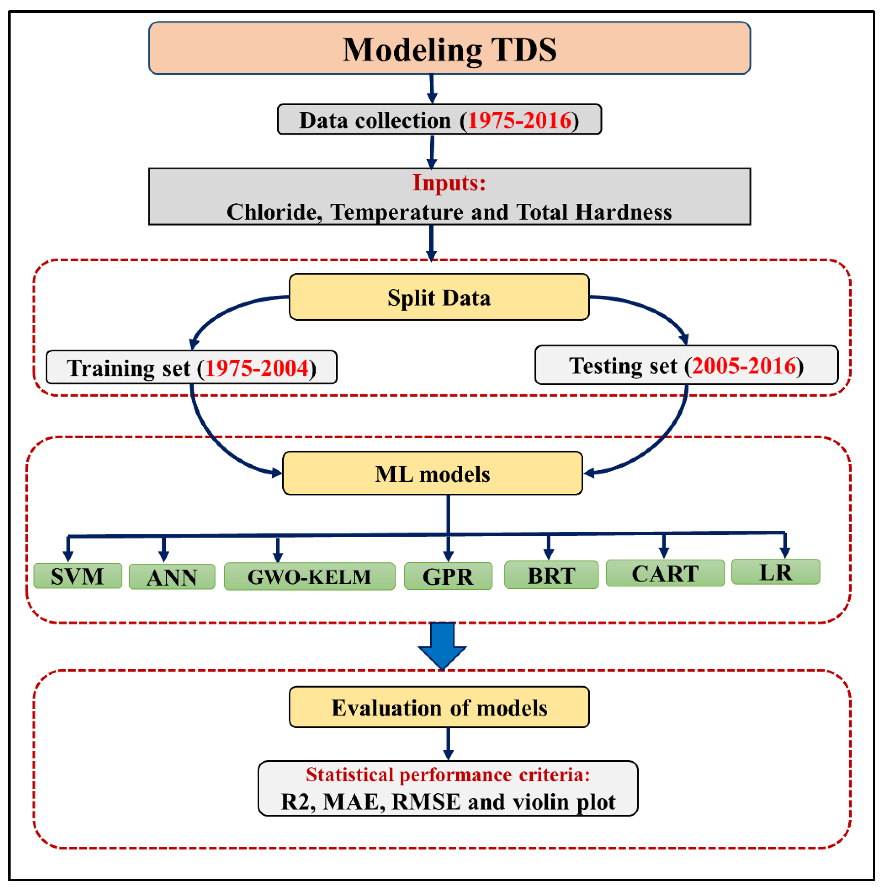
This methodology section is divided into four parts: (1) data collection and preparation, (2) driving factors; (3) machine learning algorithms, and (4) evaluation of the machine learning algorithms. Figure 2 provides a flowchart of the research method, offering a comprehensive overview of the TDS modeling steps implemented in this study.

2.2.1. Data Collection and Preparation

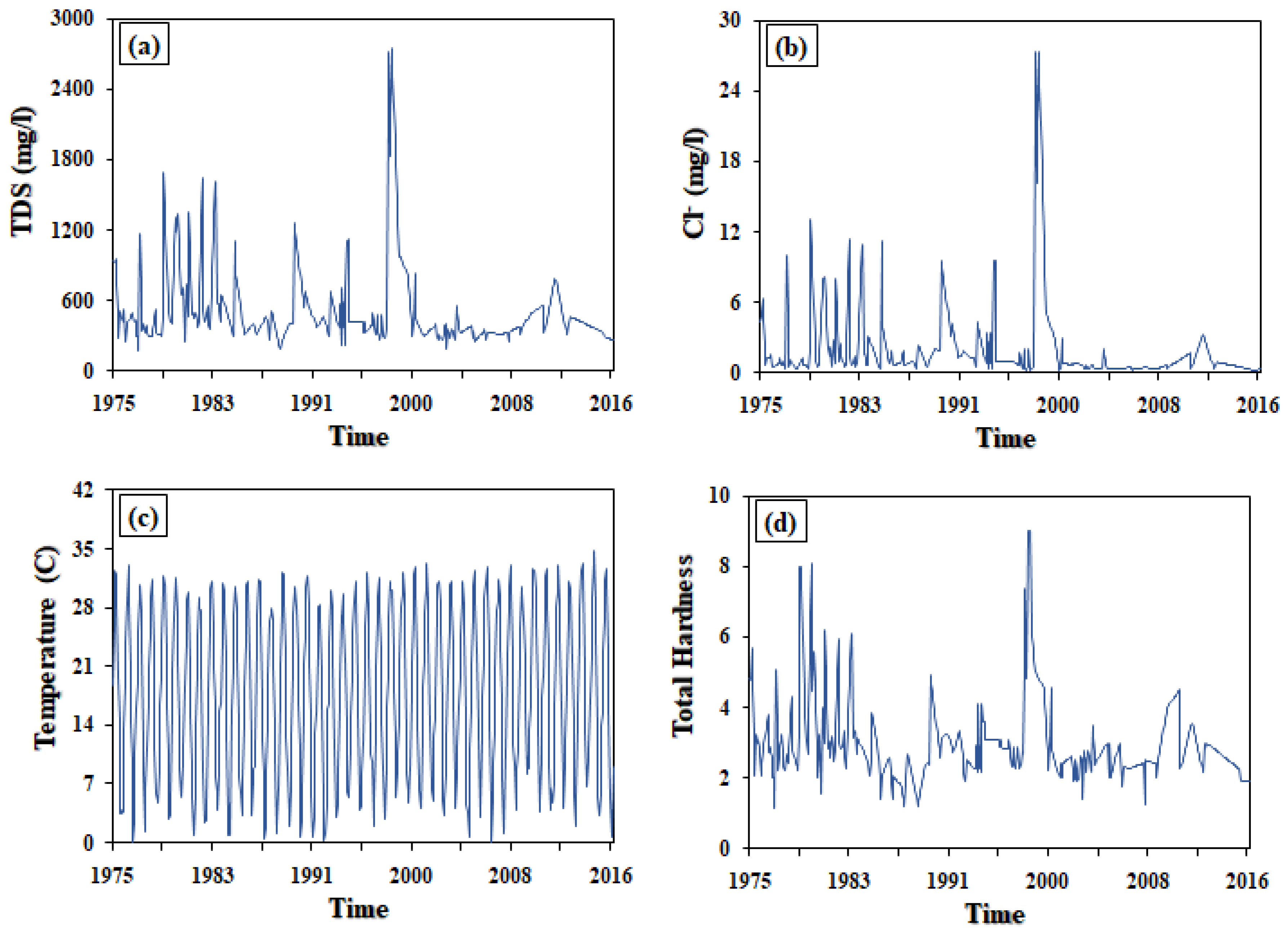
To model TDS levels, a comprehensive dataset spanning from 1975 to 2016 was compiled from reliable sources such as the West Azerbaijan Regional Water Company (WARWC) [23] and the West Azerbaijan Meteorological Organization (WAMO) [24]. This dataset includes physicochemical and climatic parameters specific to the study area. Since one of the goals of this study is to model TDS with a small number of input parameters, three parameters of chloride, total hardness, and temperature were used. This approach is particularly relevant for regions or hydrometric stations where comprehensive water quality data (including all cations, anions, and pH) are not consistently available The selected parameters were chosen due to their strong correlation with TDS and their frequent availability in most hydrometric stations. For instance, chloride and total hardness are key indicators of dissolved salts, while temperature plays a crucial role in the solubility and conductivity of ions in water. This method was inspired by previous research, such as Adjovu et al. (2023) [21], where only electrical conductivity and temperature were used successfully for TDS modeling. By reducing the number of input variables, the model has the potential to be applied in data-scarce regions, making it more practical for real-world applications where comprehensive datasets are often not available. This simplification can broaden the applicability of TDS models and provide useful insights for water quality management in resource-limited contexts. Figure 3 illustrates the time series of these parameters (Cl, TH, and temperature) from 1975 to 2016, clearly depicting their relationships as shown in Figure 3.
The purpose of using these special variables is to evaluate the efficiency of the algorithms compared to other studies that have a large number of model input parameters. The dataset from the Yalghouz Aghaj station, spanning from 1975 to 2016, was split into two subsets: a training set and a testing set. The training set, comprising 70% of the data, included records from 1975 to 2004, while the testing set, making up the remaining 30%, covered the years 2005 to 2016.

TDS

TDS is an established physical water quality parameter (WQP) recognized by the “US Environmental Protection Agency (EPA) [25]”, regulated under the “Secondary Drinking Water Regulations (SDWRs)” with a recommended maximum limit of 500 mg/L (EPA, 2018). High TDS levels could lead to damage to cooling systems, and are affected by natural origins, urban runoff, and industrial waste. Concentrations exceeding 1200 mg/L are not suitable for drinking and can affect lake mixing by increasing density gradients, which can disrupt stratification. TDS can be decomposed by microorganisms, affecting water quality. TDS is measured directly via sampling and weighing residues or indirectly through electrical conductivity (EC), which correlates with ion concentration in water. Water bodies are classified by TDS concentration into freshwater, brackish water, saline water, and brine [21,26].

2.2.2. Driving Factors

Cl

Chloride ions affect the concentration of TDS in water due to their high solubility and widespread presence. Research shows a direct correlation between chloride and TDS levels, often making chloride the major component of TDS in freshwater systems [27]. Chloride originates from natural sources such as seawater intrusion and human activities such as road deicing and industrial discharges, dissolves in water, and contributes to TDS levels. Its interactions with other ions can affect the saturation levels of minerals and influence TDS concentrations [27].

Temperature

Temperature significantly influences water conductivity and TDS levels. As water temperature increases, both conductivity and TDS also increase. This is because the movement of ions and molecules in water increases as temperature increases, leading to higher conductivity and higher TDS. In addition, temperature can affect the solubility of certain substances in water, which can also affect TDS [28]. A study by [29] analyzed the influence of temperature on TDS in different water sources, including river water, groundwater, and tap water. The study found that as the temperature increased, the TDS also increased, indicating that temperature can significantly affect the TDS of water. Therefore, it is very important to consider the temperature when measuring TDS.

Total Hardness

Total water hardness is derived from divalent cations, mainly calcium and magnesium, expressed in calcium carbonate equivalents. Specifically, 1 mg/L of calcium is equivalent to 2.5 mg/L of calcium carbonate, while 1 mg/L of magnesium is equivalent to 4.12 mg/L. In areas with high humidity, both hardness and alkalinity concentrations are often similar, while in dry areas, hardness levels usually exceed alkalinity levels. Hardness is an important factor in water quality and consumption [30]. Higher total water hardness usually increases the TDS level due to the addition of calcium and magnesium ions. The increase in TDS also depends on the presence of other substances soluble in water.

2.2.3. Machine Learning Algorithms

Support Vector Machine (SVM)

SVMs are widely recognized as kernel-based models for regression problems due to their efficiency in both classification and regression tasks. Their versatility is particularly remarkable when dealing with non-linear patterns in regression [31]. When the objective is to predict continuous variables, non-linear classifiers frequently provide more accurate results. SVMs map input data into a higher-dimensional feature space using a non-linear function and then build a linear model in that space [32]. The main advantage of SVMs lies in their ability to incorporate non-linear transformations through kernel functions, enabling them to identify complex patterns and relationships within data. This increases their performance in regression tasks involving non-linear structures [33]. In general, SVMs are very effective at handling non-linearity, making them an excellent choice for various regression challenges.
f x = ω ,   φ x + b
In this context, f(x) represents the output of the algorithm, which refers to the prediction or decision boundary. The term ω refers to the “weight vector” that determines the orientation and importance of different features in the feature space. The function ϕ(x) is a non-linear function that maps the original driving factors into a special space with higher dimensions enabling the model to capture more complex patterns. Finally, b is the bias term, which adjusts the output to better fit the data by shifting the decision boundary. In this context, a lower “w” value signifies increased flatness in Equation (2), achieved by minimizing the Euclidean norm ‖w‖. The constrained form of the SVM regression function is represented as follows:
ω i φ x i + b i d i ε + ξ i * . i = 1 .   2 .     N d i ω i φ x i b i ε + ξ i . i = 1 .   2 . .   N ξ i ξ i * 0 i = 1 .   2 . .   N
In simple terms, ξi and ξi* are variables that help handle errors, and the parameter C affects how much we allow errors and how we balance the accuracy and complexity of the model.

Artificial Neural Network (ANN)

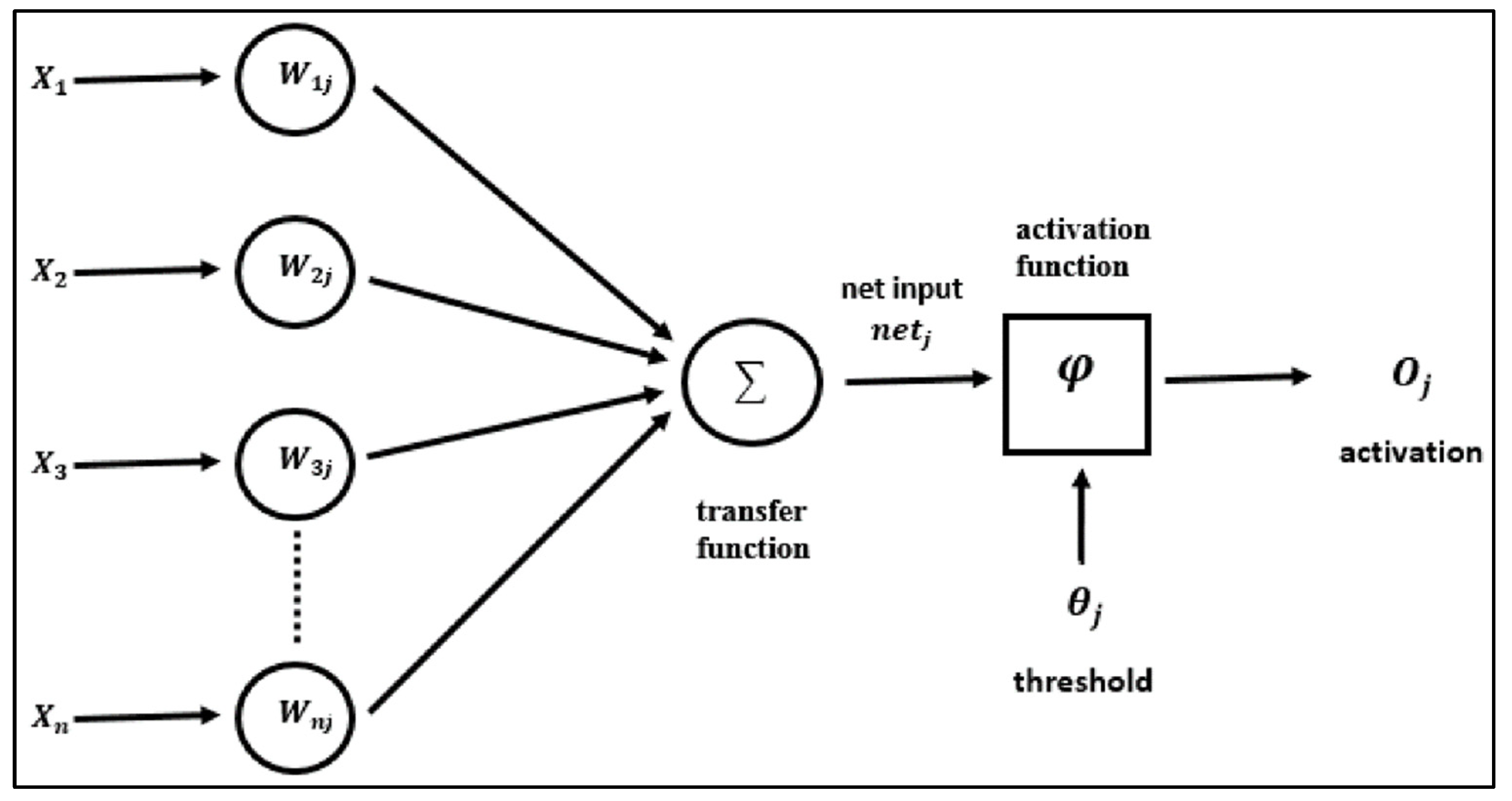
An artificial neuron serves as the fundamental building block for all ANNs, mimicking the structure and behavior of natural neurons found in biological neural networks, as described by Singh et al. (2004) [34]. The architecture of an artificial neuron, depicted in Figure 4, consists of several key components. These include input variables, which represent the data fed into the neuron, and weights, which determine the significance of each input. The neuron also incorporates transfer functions that process the weighted inputs, and activation functions that apply a non-linear transformation to the result. Additionally, a threshold is used to decide whether the neuron should be activated, and finally, the neuron produces an output based on the processed information.
An artificial neuron processes multiple inputs, where the influence of each input depends on its weight, the transfer function, and the output. Higher weights increase the impact of the corresponding inputs. The transfer function sums these weighted inputs to produce the neuron’s net input [35].
n e t j = i = 1 n ω i j x i + b
Here, j represents the specific neuron number, xi is an input value ranging from 1 to n, wij is the corresponding weight, and b is the negative threshold value, known as the neuron’s bias.
x j = φ ( u j θ j )
where xj is the output signal and θj is the bias term of the j neuron. The logistic sigmoid function, Bilgili and Yasar 2007, is used for this purpose [15] expressed as given in Equation (5).
φ x = 1 1 + e x

Gaussian Process Regression (GPR)

A Gaussian process (GP) is a collection of random variables, where any smaller group of them follows a joint multivariate Gaussian distribution. In regression, given input domain χ and output domain γ, a GP on χ is defined by a mean function μ: χ → ℝ and a covariance function (kernel). In Gaussian Process Regression (GPR), the relationship between input x and output y is modeled as y = f(x) + ξ, where f(x) is the true function and ξ is normally distributed noise with mean zero and variance σ2.
Each input x in GPR corresponds to a random variable f(x), representing the value of the random function f at that particular input. This function f is drawn from a Gaussian process, which is defined over the input domain χ. The features of this Gaussian process are shaped by its kernel function k. This function sets how much two points in the input space are related, which affects the smoothness and other traits of the function f.
This study assumes the observational error ξ is normally distributed with a mean of zero and variance σ2. The function f(x) is drawn from a Gaussian process defined on the input domain χ using the kernel function k. This kernel function plays a crucial role in determining how different input points are related and ultimately influences the predictions made by the GPR model [36].

Boosted Regression Tree (BRT)

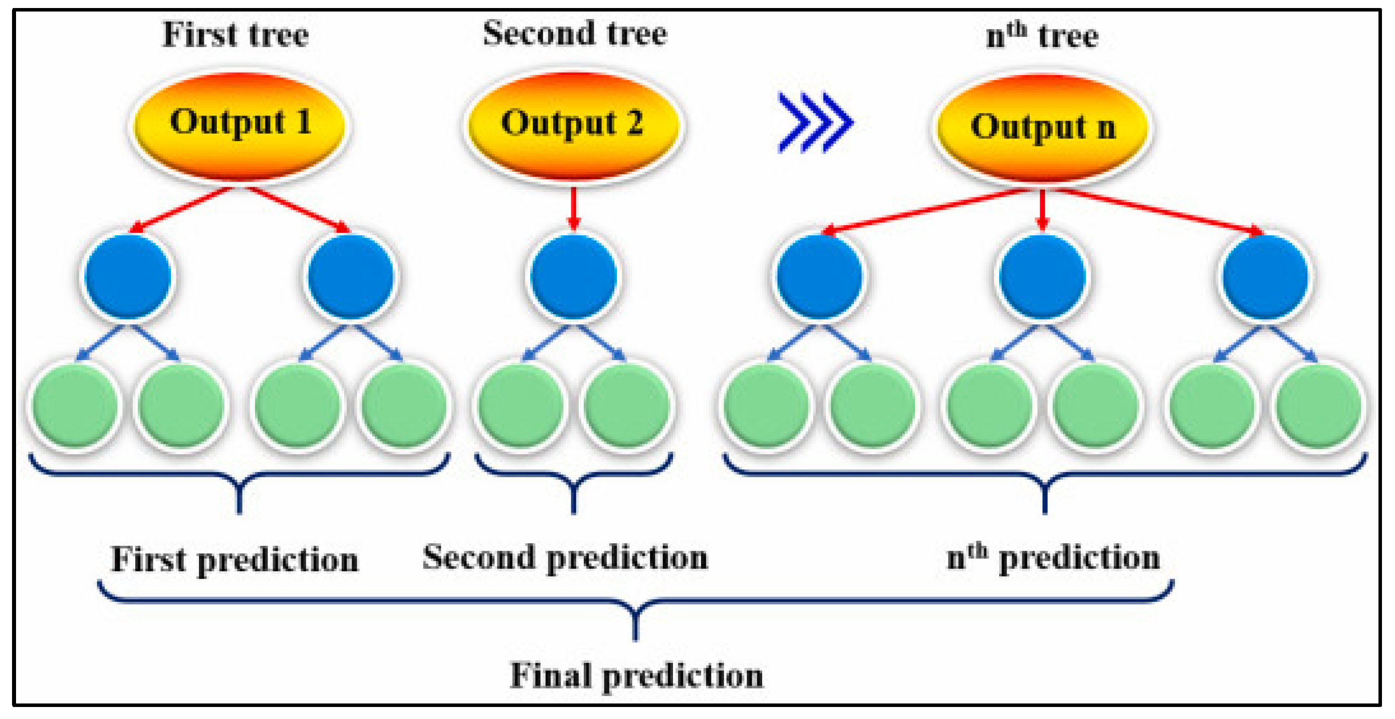
Ensembles, especially those utilizing tree-based models, represent some of the most versatile and valuable approaches in machine learning [37]. These ensembles consist of multiple trained models whose predictions are combined to improve overall predictive performance. This category of machine learning encompasses various methodologies, with bagging and boosting standing out as the most prominent and well known [38]. Bagging techniques, abbreviated for “bootstrap aggregating”, involve training multiple learners independently in parallel. The aim is to create an ensemble model that surpasses the resilience of its individual components [39]. The process is straightforward: numerous bootstrap samples are generated from the original dataset, each sample undergoes predictive modeling, and the results are averaged for regression to obtain the final prediction, reducing variance through averaging [40]. Boosted regression trees (BRTs), akin to Random Forest models, iteratively fit numerous decision trees to enhance model accuracy. A distinguishing feature between these approaches is how tree-generation data are selected. Both methods employ random subsets of the entire dataset for each new tree [41]. These subsets mirror the full dataset’s size, with data reused across trees. BRTs adopt a boosting approach where successive tree data inputs are weighted, prioritizing data poorly approximated by earlier trees to refine subsequent models [42]. This sequential boosting strategy is distinctive, continuously striving to improve accuracy by building upon prior tree fits [43]. Critical parameters for BRTs include tree complexity (Tc) and learning rate (lr). Tc governs the number of splits per tree: a Tc of 1 yields trees with only one split, neglecting environmental factor interactions, while higher values allow for more splits [38]. The lr determines each tree’s contribution to the evolving model, with lower values necessitating more trees for model construction. Optimizing Tc and lr involves balancing these factors to minimize prediction errors, typically targeting at least 1000 trees for robust models, with optimal settings contingent on dataset characteristics [44]. Figure 5 depicts the typical configuration of BRTs.
The colored circles in the figure represent various values of the output parameter (TDS) and the input parameters (chloride, total hardness, and temperature). The colors help in distinguishing the relationships between these parameters. Specifically:
  • Red circles indicate higher TDS levels in conjunction with higher chloride concentrations.
  • Green circles signify moderate TDS values, corresponding to medium levels of total hardness.
  • Blue circles represent lower TDS values and lower temperatures, highlighting areas with reduced solubility or changes in water chemistry.

Classification and Regression Tree (CART) Algorithm

Tree-based methods use decision trees to make predictions or decisions. In a decision tree, the root node represents the whole dataset, and the child nodes show data splits based on conditions [46]. CART, a widely used decision tree algorithm introduced by Breiman in 1984 [47], is applicable to both classification and regression tasks. For regression tasks like predicting soil water content (SWC), CART splits data based on features and thresholds to minimize the sum of squared errors (SSE) [48]. For a dataset with N observations, p features, and one response variable, minimizing SSE for a split can be mathematically expressed as follows:
m i n j ,   s   [ m i n c L x i R L j , s y i c L 2 + m i n c R x i R R j , s y i c R 2   ]
In this equation, xi = (xi(1), xi(2), …, xi(p)) represents the input features, and yi is the target feature for the i-th observation. R denotes a subset of the dataset at a given split, with RL and RR indicating the left and right branches. CL and CR are the average responses in these branches. The goal is to find the feature j and threshold s that best split the data into distinct subgroups.

Linear Regression (LR)

LR is a common algorithm for analyzing variable relationships in prediction tasks, assuming a linear relationship between inputs and the response variable. It estimates coefficients to minimize the sum of squared errors (SSE). LR models are uncomplicated yet potent tools for making decisions. A key hyperparameter in LR is the regularization parameter α, which balances model complexity and prevents overfitting. Regularization techniques, such as ridge regression, preserve the significance of predictors by applying penalties, while LASSO encourages model simplicity by dropping less significant coefficients to zero. Adjusting these parameters controls the model’s regularization strength and its sensitivity to outliers. In this study, ordinary least squares (OLS) regression was used, which minimizes the squared errors between observed and predicted values without penalty coefficients [49]. Linear regression models can be simple, including one predictor, or multiple, including several predictors to predict the response variable [50].

Kernel Extreme Learning Machine (KELM)

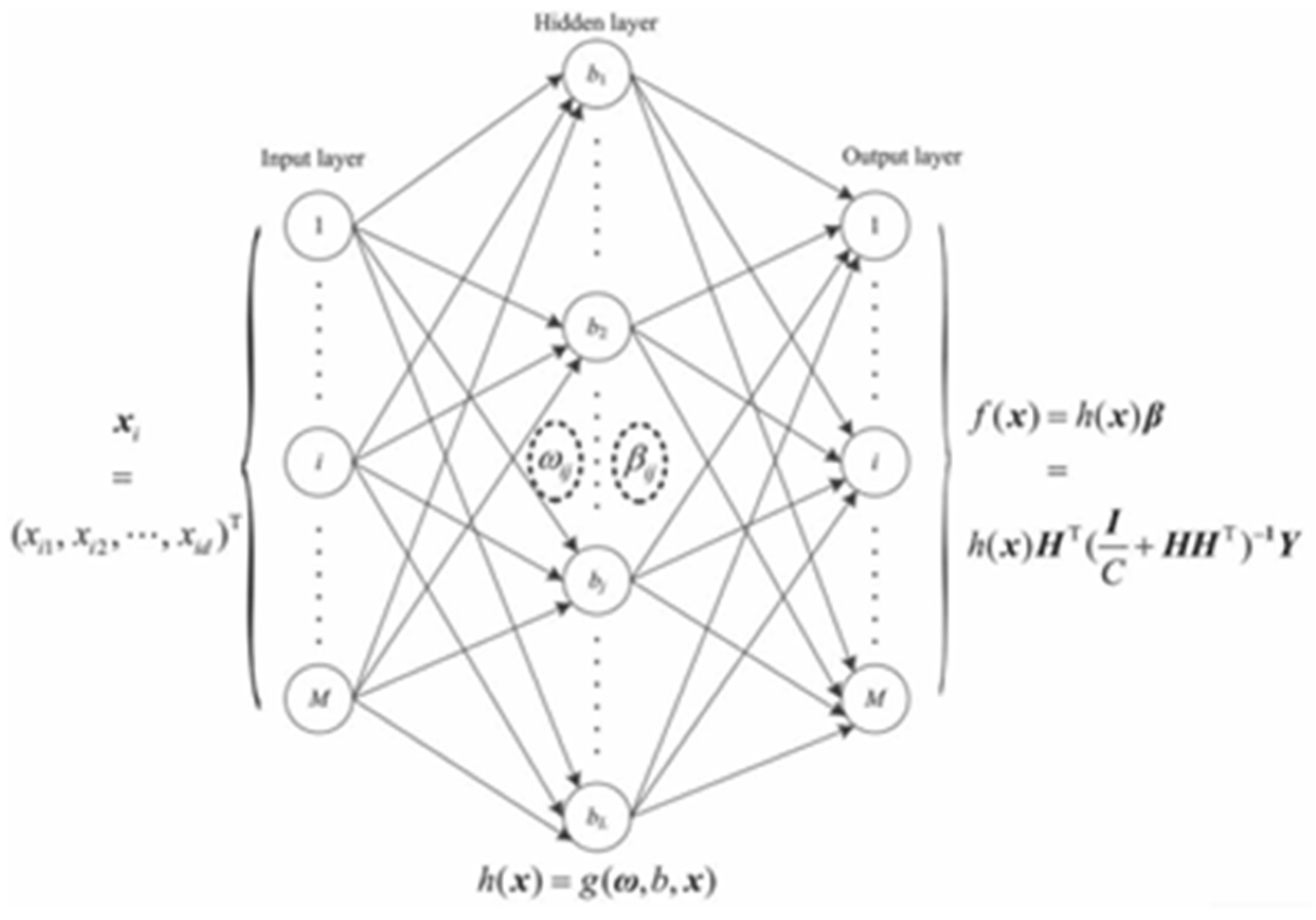
An ELM is a type of neural network with just one hidden layer, as shown by Huang et al. Unlike traditional neural networks, which require tweaking many parameters and often end up with less-than-ideal solutions, ELMs are simpler to use. You only need to decide how many hidden nodes you want, and you do not have to adjust the input weights or hidden layer biases. This makes it easier to find the best solution quickly. As a result, ELMs learn faster and perform better [51]. The structure of an ELM is shown in Figure 6.

Grey Wolf Optimization (GWO)

Inspired by the social structure and hunting tactics of grey wolves, Mirjalili [53] created the GWO algorithm as a new metaheuristic method. It is based on two main behaviors: the hierarchical system, with alpha (α) wolves at the top as leaders (shown in Figure 7), and hunting behavior. GWO is used in fields like water engineering, parameter optimization, and image classification [54]. In this study, GWO helps find the best KELM hyperparameters (kernel parameters and regularization coefficient), with the algorithm’s process mimicking wolf hunting, where the prey represents the optimized parameters. The first step involves updating the wolves’ positions in relation to the prey.

2.2.4. Evaluation of the Machine Learning Algorithms

To assess how well machine learning algorithms perform in modeling TDS values, various statistical measures were used, including R2, RMSE, and MAE. R2 measures how well the independent variables (such as total hardness, temperature, and chloride) explain the variance in the dependent variable TDS, with values ranging from −∞ to 1 [55]. Higher R2 values (approximately 0.75 to 1.00) indicate robustness and correlation between observed and predicted values, while values less than 0.4 indicate poor performance of the model in explaining the variability of the data [21]. RMSE, sensitive to larger errors, measures model fit, with an ideal model having zero RMSE [18]. MAE evaluates forecast accuracy by calculating the mean absolute difference between predicted and observed values, ignoring their signs [56]. Below are the equations for R2, RMSE, and MAE:
R 2 = 1 i = 1 n T D S p r e d T D S o b s 2 i = 1 n T D S ¯ o b s T D S o b s 2
R M S E = i = 1 n ( T D S o b s T D S p r e d ) 2 n
M A E = 1 n i = 1 n T D S o b s T D S p r e d
where TDSobs, TDSpred, T D S ¯ o b s , and T D S ¯ p r e d are the observed, predicted, average of observed, and average of predicted values, respectively.
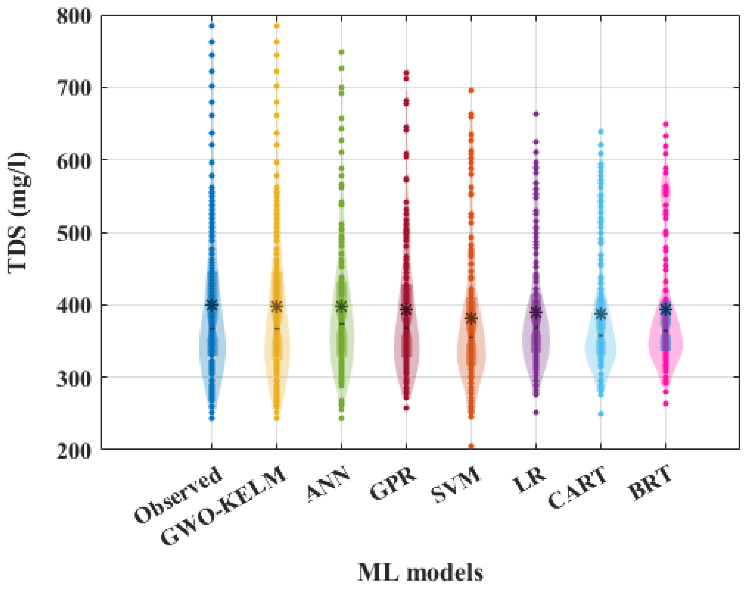
Moreover, in this study, the violin plot graphic method was used to show the superior model. A violin plot combines features of a box plot and a kernel density plot to give a detailed view of a dataset’s distribution. It displays the distribution’s probability density at different values, giving a clear indication of where data points are concentrated. The central part of the plot shows the median and interquartile range, similar to a box plot, while the sides of the “violin” shape illustrate the density of the data across the range of values, often with a smooth, mirrored curve. This makes violin plots particularly useful for comparing distributions across multiple groups, highlighting differences in their spread, skewness, and central tendency [57].

3. Results and Discussion

The statistical Table 1 presents essential parameters pertinent to TDS modeling in water quality assessment. The average TDS concentration is 510 mg/L, with a significant range from 166 mg/L to 2752 mg and a standard deviation of 337 mg/L, indicating considerable variability. Chloride levels average 2 mg/L, ranging from 0.2 mg/L to 27 mg/L, with a standard deviation of 3.36 mg/L, reflecting moderate variability. Temperature data show an average of 17.65 °C, spanning from 0 °C to 34.70 °C, with a standard deviation of 10 °C, highlighting substantial seasonal and environmental fluctuation. Total hardness averages 2.97, ranging from 1.15 to 10.10, with a standard deviation of 1.10, indicating varying mineral content across samples. These statistics are pivotal for understanding the distribution and variability of key parameters impacting water quality, crucial for scientific research and environmental management strategies.

3.1. Results of ML Algorithms

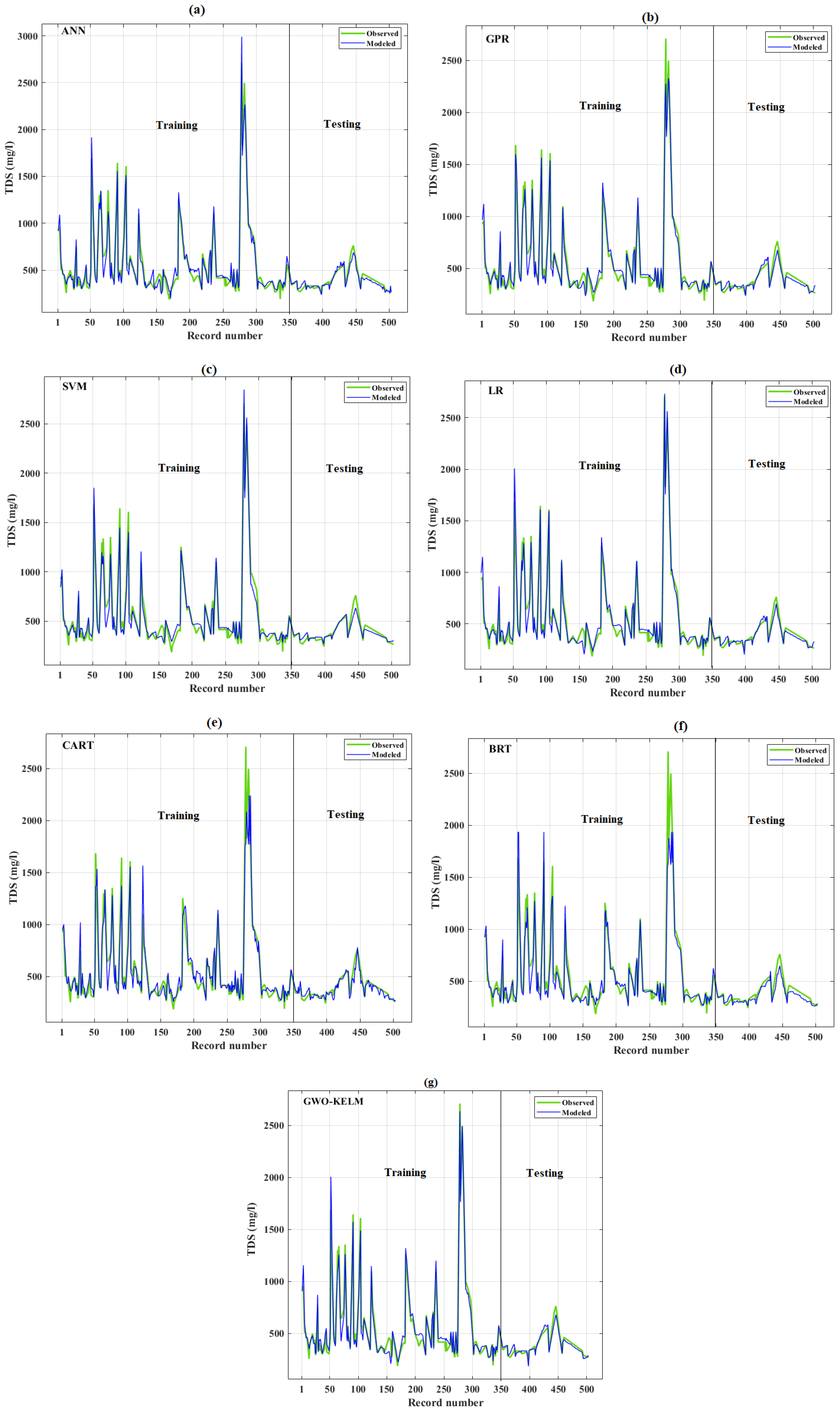
The ANN model, designed for modeling TDS using temperature, total hardness, and chloride, demonstrated outstanding performance (Figure 8a). With an R2 of 0.969, it indicated a strong correlation between predicted and actual TDS values. The model also achieved an MAE of 38 and an RMSE of 40, showcasing its exceptional accuracy and precision in TDS modeling (Table 2). The GPR model, utilizing temperature, total hardness, and chloride to model TDS, showed excellent performance (Figure 8b). It achieved a high R2 of 0.962, meaning it explained 96% of the variance in TDS. The model’s MAE was 40, and its RMSE was 65, reflecting its strong accuracy in TDS predictions (Table 2).
The SVM model, which also used temperature, total hardness, and chloride for modeling TDS, demonstrated strong performance (see Figure 8c). It had an R2 of 0.959, indicating robust estimation of TDS values. The MAE and RMSE were 42 and 69, respectively (Table 2), highlighting its effectiveness in accurately estimating TDS despite data complexities. The LR model, developed for TDS prediction with temperature, total hardness, and chloride, exhibited good performance (Figure 8d). It achieved an R2 of 0.953, showing satisfactory efficiency in predicting TDS values. The MAE and RMSE were 44 and 74, respectively (Table 2), indicating its reasonable accuracy. The linear equation for this model is:
y = 0.7411 x + 90.827
The CART model, designed to model TDS using temperature, total hardness, and chloride, displayed satisfactory performance (Figure 8e). It obtained an R2 of 0.908, demonstrating its capability to predict TDS values effectively. The MAE and RMSE were 55 and 102, respectively (Table 2), reflecting its reasonable accuracy. The BRT model, which used temperature, total hardness, and chloride for TDS prediction, showed effective performance (Figure 8f). It achieved an R2 of 0.895, indicating a strong correlation between predicted and actual TDS values. The MAE and RMSE were 53 and 108, respectively (Table 2), demonstrating its good accuracy in predicting TDS levels. The GWO-KELM model, utilizing temperature, total hardness, and chloride for TDS prediction, delivered excellent performance (Figure 8g). It achieved a high R2 of 0.974, indicating a very strong relationship between predicted and actual TDS values. With an MAE of 34.40 and an RMSE of 55.75 (Table 2), this model demonstrated high accuracy in TDS predictions. It has also been noted for its superior performance in other studies, such as predicting discharge coefficients in submerged radial gates [54].

3.2. Graphical Results

This study focused on TDS modeling using seven different machine learning algorithms: GWO-KELM, ANN, GPR, SVM, LR, CART, and BRT. To evaluate and compare the performance of these models, violin plots were used to visualize the distribution of their predictive accuracies (Figure 9). Violin plots provide a detailed view of the distribution of a dataset. Unlike standard box plots, violin plots also display the density of the data across different values, which helps in understanding the distribution more comprehensively. Each violin plot represents the distribution of predictive accuracies for one model, showing how frequently certain accuracy levels occur and how these levels are distributed. The asterisks (*) are used to mark statistically significant data points or results, which highlight areas where [insert reason for significance, such as critical thresholds, outliers, or notable changes in trends]. These are critical for emphasizing deviations or important results in [specific analysis or model behavior]. Specifically, * indicates a value that has exceeded [a particular threshold or parameter], showcasing [why these points are relevant].
In the violin plots, the shape of the violin plot reflects the density of predictive accuracies. A wider section of the plot indicates a higher density of data points at that accuracy level. If a model’s violin plot is wider and more centered, it suggests that this model consistently achieves higher predictive accuracy and has a stable performance. The central part of the violin plot represents the median or central tendency of the predictive accuracies. A model with a violin plot that has a higher central peak generally performs better on average. By comparing the shapes and central tendencies of the violin plots for all models, the GWO-KELM model was identified as the superior performer. Its violin plot exhibited a more favorable distribution shape, indicating that it consistently achieved higher accuracy compared to the other models. The central peak of the GWO-KELM plot was higher, and the distribution was more concentrated around this peak, demonstrating its better overall performance.
While the GWO-KELM model showed superior performance, the violin plots for other models also showed similar shapes and overlapping distributions. This overlap suggests that although GWO-KELM was the top performer, the other models also performed well and had comparable predictive power. Overall, the violin plots effectively highlight the differences in performance among the models. The clear and distinct shape of the GWO-KELM plot, with its higher and more concentrated central tendency, underscores its role as the most accurate model in this study. The ability to visualize both the distribution and density of predictive accuracies provides a clear rationale for selecting the best-performing model.

3.3. Discussion of ML Algorithms’ Performance

Upon comparing seven modeling approaches (GWO-KELM, ANN, SVM, GPR, LR, CART, and BRT) for TDS prediction using temperature, total hardness, and chloride parameters, the GWO-KELM emerged as the top performer with the highest R2 value of 0.974. This indicates the strongest correlation between predicted and actual TDS values, accompanied by low MAE and RMSE, reflecting its superior accuracy and precision in capturing complex relationships within the data. Following closely, the ANN model achieved an R2 of 0.968, demonstrating its robust performance in modeling TDS levels with high accuracy and providing probabilistic predictions. GPR also showed strong performance with an R2 of 0.962. The LR, CART, and BRT models differed by 0.02, 0.07, and 0.08, respectively, with the GWO-KELM model, which indicates the close competition of machine learning models in TDS modeling in this study.
The GWO-KELM model outperformed other methods in TDS modeling due to its hybrid nature, combining GWO’s efficient global optimization with KELM’s ability to capture complex non-linear relationships. This combination enhances model accuracy, robustness to noise, and computational efficiency, making it superior to benchmark methods like ANN, SVM, and others that may struggle with optimization challenges, noise, or computational demands. The GWO’s capability to avoid local optima and KELM’s flexibility in non-linear mapping contribute significantly to its effectiveness in modeling water quality parameters [54]. The ANN’s capability to adapt and refine its predictions through continuous learning enhances its applicability in environmental monitoring and management, contributing significantly to informed decision making and resource management strategies. The high accuracy of the GPR model can be attributed to its ability to capture complex, non-linear relationships between the inputs and the target variable through its flexible, non-parametric structure, which enables it to learn intricate patterns in the data without assuming a specific form for the underlying function. This adaptability allows the GPR model to effectively generalize to new data and provide reliable forecasts of TDS concentrations across diverse environmental conditions, thereby supporting informed decision making in environmental monitoring and management practices [58]. ANNs have an edge over SVMs in modeling environmental data like TDS because they can capture more complex, non-linear relationships and handle larger datasets more effectively. ANNs are also less reliant on manual feature engineering and can be scaled easily by adjusting their architecture, making them adaptable to various problem sizes. Additionally, ANNs benefit from parallel processing on modern hardware, allowing for faster training and predictions compared to SVMs [59,60]. While the LR model is slightly less accurate than the more complex ANN, SVM, and GPR models, it still provides reliable predictions, showcasing its simplicity and effectiveness in modeling TDS with these key environmental factors. The LR model’s straightforward approach leverages linear relationships between variables, offering a clear interpretation of how changes in temperature, total hardness, and chloride impact TDS levels, thereby supporting practical applications in environmental monitoring and management [61,62]. The CART model was generally weaker than the ANN, GPR, and SVM models for TDS modeling because it often struggles with capturing more complex, non-linear relationships and interactions in the data. While CART can handle non-linearity to some extent, its decision tree structure is less flexible and less capable of learning intricate patterns compared to ANN’s deep learning layers, GPR’s probabilistic approach, and SVMs [60]. These more advanced models can better accommodate high-dimensional data and complex interactions, leading to more accurate and robust predictions for TDS.
BRT models excel in capturing complex interactions and non-linearities within data, leveraging the boosting technique to iteratively improve predictions. Despite being slightly less accurate than some other advanced models like ANN or SVM, the BRT model remains a strong choice for TDS prediction due to its robustness and ability to handle diverse environmental data effectively. The ensemble nature of BRT allows it to combine the strengths of multiple weak learners, enhancing predictive performance while maintaining interpretability through feature importance rankings, thereby supporting informed decision making in environmental monitoring and management contexts.
Table 3 summarizes the primary previous works in TDS modeling. As seen in Table 3, researchers have used a wide range of physicochemical parameters to model TDS in water. These parameters often include various chemical concentrations, pH levels, and other water quality indicators. However, in this present study, it only focused on three specific parameters: chloride, temperature, and total hardness. These were used as input parameters for machine learning models. It is noteworthy that despite the reduction in the number of parameters, the models in this study achieved the same level of assessment accuracy as in previous studies that used a wider set of parameters. This result emphasizes the critical importance of carefully selecting appropriate input parameters for TDS modeling. Correct selection of these parameters is essential and can significantly affect model performance, suggesting that a well-considered choice can simplify the modeling process without compromising accuracy.

4. Conclusions

This study aimed to model TDS using various machine learning methods, including GWO-KELM, SVM, ANN, GPR, LR, BRT, and CART. Three parameters—chloride, temperature, and total hardness—were used as input features for the machine learning models. The results demonstrated that the GWO-KELM model, with an outstanding R² value of 0.974, an MAE of 34.40, and an RMSE of 55.75, effectively modeled TDS. The superior performance of the GWO-KELM model can be attributed to its hybrid nature, which combines the strengths of the GWO algorithm and KELM.
The GWO algorithm is a nature-inspired optimization technique that mimics the hunting strategy of grey wolves. In this context, GWO is used to optimize the hyperparameters of the KELM model, such as kernel parameters and the regularization coefficient, which are crucial for enhancing the model’s performance. By efficiently searching the hyperparameter space, GWO avoids the pitfalls of manual tuning and helps the model achieve better generalization. On the other hand, KELM is known for its fast learning speed and capability to handle complex, non-linear relationships in the data through the use of a kernel function. However, the success of KELM heavily depends on the selection of optimal hyperparameters, where GWO optimization plays a crucial role. The combination of GWO’s effective optimization strategy with KELM’s strong learning capabilities results in a model that not only captures intricate patterns in the input data but also minimizes error more effectively than other models. This hybrid approach explains why the GWO-KELM model outperformed other machine learning models such as ANN and GPR. While these models rely on internal mechanisms for learning (e.g., ANN can be prone to getting stuck in local minima), the GWO-KELM model’s ability to dynamically adjust its hyperparameters allows it to achieve higher accuracy and lower error rates, as reflected in its R2 value of 0.974 and low MAE and RMSE values. Thus, the combination of GWO’s optimization capabilities and KELM’s efficient learning process makes GWO-KELM the most effective model for TDS prediction in this study.
Additionally, this study used fewer factors yet achieved strong performance compared to other studies with more comprehensive datasets. This makes the current framework more generalizable and feasible, especially for data-scarce regions. Overall, this study highlights the potential of cost-effective machine learning approaches to model TDS in water using total hardness, chloride, and temperature as inputs.
To improve the accuracy of the TDS model, several strategies can be applied. Feature engineering, by incorporating additional water quality or climate data, can help capture complex relationships. Handling seasonality through techniques like time series decomposition and employing advanced hyperparameter tuning methods such as Bayesian optimization can refine the model’s performance. Ensemble methods like Random Forest or Gradient Boosting, combined with cross-validation, will enhance robustness. Further data preprocessing, such as normalization, and exploring deep learning models like LSTM for temporal data can also improve accuracy. Incorporating more recent datasets, if available, would further strengthen predictions.

Author Contributions

M.S.: data curation, formal analysis, investigation, methodology, validation, visualization, writing—original draft, writing—review and editing. B.H.: data curation, review and editing. M.M.: review and editing. A.N.: conceptualization, formal analysis, investigation, methodology, validation, writing—review and editing. All authors have read and agreed to the published version of the manuscript.

Funding

This research received no external funding.

Data Availability Statement

Data available on request due to restrictions eg privacy or ethical. The data presented in this study are available on request from the corresponding author. The data are not publicly available due to the confidentiality of water quality data of Urmia Lake catchment.

Acknowledgments

The authors greatly appreciate the facility support provided by the division of water resources engineering, Lund University.

Conflicts of Interest

The authors declare that they have no known competing financial interests or personal relationships that could have appeared to influence the work reported in this paper.

Abbreviations

AbbreviationsDescription
TDSTotal Dissolved Solids
GWOGrey Wolf Optimization
KELMKernel Extreme Learning Machine
ELMExtreme Learning Machine
ANNArtificial Neural Network
GPRGaussian Process Regression
SVMSupport Vector Machine
LRLinear Regression
CARTClassification and Regression Tree
BRTBoosted Regression Tree
R2Coefficient of determination
RMSERoot Mean Square Error
MAEMean Absolute Error
MLMachine learning
THTotal hardness
WARWCWest Azerbaijan Regional Water Company
WAMOWest Azerbaijan Meteorological Organization
WQPWater quality parameter
EPAEnvironmental Protection Agency
SDWRsSecondary Drinking Water Regulations
GPGaussian process
SWCSoil Water Content

References

  1. Karimi, S.; Amiri, B.J.; Malekian, A. Similarity metrics-based uncertainty analysis of river water quality models. Water Resour. Manag. 2019, 33, 1927–1945. [Google Scholar] [CrossRef]
  2. Bui, D.T.; Khosravi, K.; Tiefenbacher, J.; Nguyen, H.; Kazakis, N. Improving prediction of water quality indices using novel hybrid machine-learning algorithms. Sci. Total Environ. 2020, 721, 137612. [Google Scholar] [CrossRef] [PubMed]
  3. Sun, K.; Rajabtabar, M.; Samadi, S.; Rezaie-Balf, M.; Ghaemi, A.; Band, S.S.; Mosavi, A. An integrated machine learning, noise suppression, and population-based algorithm to improve total dissolved solids prediction. Eng. Appl. Comput. Fluid Mech. 2021, 15, 251–271. [Google Scholar] [CrossRef]
  4. Zounemat-Kermani, M.; Seo, Y.; Kim, S.; Ghorbani, M.A.; Samadianfard, S.; Naghshara, S.; Kim, N.W.; Singh, V.P. Can decomposition approaches always enhance soft computing models? Predicting the dissolved oxygen concentration in the St. Johns River, Florida. Appl. Sci. 2019, 9, 2534. [Google Scholar] [CrossRef]
  5. Butler, B.A.; Ford, R.G. Evaluating relationships between total dissolved solids (TDS) and total suspended solids (TSS) in a mining-influenced watershed. Mine Water Environ. 2018, 37, 18. [Google Scholar] [CrossRef]
  6. Adjovu, G.E.; Stephen, H.; James, D.; Ahmad, S. Measurement of total dissolved solids and total suspended solids in water systems: A review of the issues, conventional, and remote sensing techniques. Remote Sens. 2023, 15, 3534. [Google Scholar] [CrossRef]
  7. Wen, Z.; Han, J.; Shang, Y.; Tao, H.; Fang, C.; Lyu, L.; Li, S.; Hou, J.; Liu, G.; Song, K. Spatial variations of DOM in a diverse range of lakes across various frozen ground zones in China: Insights into molecular composition. Water Res. 2024, 252, 121204. [Google Scholar] [CrossRef]
  8. Mahmoodlu, M.G.; Jandaghi, N.; Sayadi, M. Investigating the factors affecting corrosion and precipitation changes along Gorganroud River, Golestan Province. Environ. Sci. 2021, 19, 71–90. [Google Scholar] [CrossRef]
  9. Banadkooki, F.B.; Ehteram, M.; Panahi, F.; Sammen, S.S.; Othman, F.B.; Ahmed, E.S. Estimation of total dissolved solids (TDS) using new hybrid machine learning models. J. Hydrol. 2020, 587, 124989. [Google Scholar] [CrossRef]
  10. Liu, S.; Qiu, Y.; He, Z.; Shi, C.; Xing, B.; Wu, F. Microplastic-derived dissolved organic matter and its biogeochemical behaviors in aquatic environments: A review. Crit. Rev. Environ. Sci. Technol. 2024, 54, 865–882. [Google Scholar] [CrossRef]
  11. Sayadi, M.; Mahmoodlu, M.G. Investigation and prediction of quality parameters of Gamasyab river using multivariate method of Canonical correlation analysis and time series. J. Res. Environ. Health 2019, 5, 108–122. [Google Scholar]
  12. Yang, H.; Kong, J.; Hu, H.; Du, Y.; Gao, M.; Chen, F. A review of remote sensing for water quality retrieval: Progress and challenges. Remote Sens. 2022, 14, 1770. [Google Scholar] [CrossRef]
  13. Adjovu, G.; Ahmad, S.; Stephen, H. Analysis of Suspended Material in Lake Mead Using Remote Sensing Indices. In Proceedings of the World Environmental and Water Resources Congress 2021, Online, 7–11 June 2021; pp. 754–768. [Google Scholar]
  14. Dritsas, E.; Trigka, M. Efficient data-driven machine learning models for water quality prediction. Computation 2023, 11, 16. [Google Scholar] [CrossRef]
  15. Al-Mukhtar, M.; Al-Yaseen, F. Modeling water quality parameters using data-driven models, a case study Abu-Ziriq marsh in south of Iraq. Hydrology 2019, 6, 24. [Google Scholar] [CrossRef]
  16. Ewusi, A.; Ahenkorah, I.; Aikins, D. Modelling of total dissolved solids in water supply systems using regression and supervised machine learning approaches. Appl. Water Sci. 2021, 11, 13. [Google Scholar] [CrossRef]
  17. Panahi, J.; Mastouri, R.; Shabanlou, S. Influence of pre-processing algorithms on surface water TDS estimation using artificial intelligence models: A case study of the Karoon river. Iran. J. Sci. Technol. Trans. Civ. Eng. 2023, 47, 585–598. [Google Scholar] [CrossRef]
  18. Pourhosseini, F.A.; Ebrahimi, K.; Omid, M.H. Prediction of total dissolved solids, based on optimization of new hybrid SVM models. Eng. Appl. Artif. Intell. 2023, 126, 106780. [Google Scholar] [CrossRef]
  19. Hijji, M.; Chen, T.C.; Ayaz, M.; Abosinnee, A.S.; Muda, I.; Razoumny, Y.; Hatamiafkoueieh, J. Optimization of state of the art fuzzy-based machine learning techniques for total dissolved solids prediction. Sustainability 2023, 15, 7016. [Google Scholar] [CrossRef]
  20. Melesse, A.M.; Khosravi, K.; Tiefenbacher, J.P.; Heddam, S.; Kim, S.; Mosavi, A.; Pham, B.T. River water salinity prediction using hybrid machine learning models. Water 2020, 12, 2951. [Google Scholar] [CrossRef]
  21. Adjovu, G.E.; Stephen, H.; Ahmad, S. A machine learning approach for the estimation of total dissolved solids concentration in lake mead using electrical conductivity and temperature. Water 2023, 15, 2439. [Google Scholar] [CrossRef]
  22. Roushangar, K.; Aalami, M.T.; Golmohammadi, H.; Shahnazi, S. Monitoring and prediction of land use/land cover changes and water requirements in the basin of the Urmia Lake, Iran. Water Supply 2023, 23, 2299–2312. [Google Scholar] [CrossRef]
  23. West Azarbaijan Regional Water Company. Available online: https://www.agrw.ir/ (accessed on 10 May 2023).
  24. West Azerbaijan Meteorological Organization. Available online: http://www.azmet.ir/ (accessed on 10 May 2023).
  25. U.S. EPA. 2018 Edition of the Drinking Water Standards and Health Advisories Tables; U.S. EPA: Washington, DC, USA, 2018. Available online: https://www.epa.gov/system/files/documents/2022-01/dwtable2018.pdf (accessed on 25 May 2023).
  26. Rusydi, A.F. February. Correlation between conductivity and total dissolved solid in various type of water: A review. IOP Conf. Ser. Earth Environ. Sci. 2018, 118, 012019. [Google Scholar] [CrossRef]
  27. Das, C.R.; Das, S.; Panda, S. Groundwater quality monitoring by correlation, regression and hierarchical clustering analyses using WQI and PAST tools. Groundw. Sustain. Dev. 2022, 16, 100708. [Google Scholar] [CrossRef]
  28. Dewangan, S.K.; Shrivastava, S.; Kadri, M.; Saruta, S.; Yadav, S.; Minj, N. Temperature effect on electrical conductivity (EC) & total dissolved solids (TDS) of water: A review. Int. J. Res. Anal. Rev 2023, 10, 514–520. [Google Scholar]
  29. Chen, J.; Wu, H.; Qian, H.; Gao, Y. Assessing nitrate and fluoride contaminants in drinking water and their health risk of rural residents living in a semiarid region of Northwest China. Expo. Health 2017, 9, 183–195. [Google Scholar] [CrossRef]
  30. Boyd, C.E. Total hardness. In Water Quality: An Introduction; Springer: Cham, Switzerland, 2015; pp. 179–187. [Google Scholar]
  31. Roushangar, K.; Shahnazi, S.; Mehrizad, A. Data-intelligence approaches for comprehensive assessment of discharge coefficient prediction in cylindrical weirs: Insights from extensive experimental data sets. Measurement 2024, 233, 114673. [Google Scholar] [CrossRef]
  32. Vapnik, V. The Nature of Statistical Learning Theory; Springer: New York, NY, USA, 1995. [Google Scholar]
  33. Roushangar, K.; Davoudi, S.; Shahnazi, S. Temporal prediction of dissolved oxygen based on CEEMDAN and multi-strategy LSTM hybrid model. Environ. Earth Sci. 2024, 83, 158. [Google Scholar] [CrossRef]
  34. Singh, K.P.; Malik, A.; Mohan, D.; Sinha, S. Multivariate statistical techniques for the evaluation of spatial and temporal variations in water quality of Gomti River (India)—A case study. Water Res. 2004, 38, 3980–3992. [Google Scholar] [CrossRef]
  35. Haykin, S. Kalman Filtering and Neural Networks; John Wiley & Sons: Hoboken, NJ, USA, 2004. [Google Scholar]
  36. Roushangar, K.; Shahnazi, S. Prediction of sediment transport rates in gravel-bed rivers using Gaussian process regression. J. Hydroinformatics 2020, 22, 249–262. [Google Scholar] [CrossRef]
  37. Kern, C.; Klausch, T.; Kreuter, F. Tree-based machine learning methods for survey research. In Survey Research Methods; NIH Public Access: Milwaukee, WI, USA, 2019; Volume 13, No. 1, p. 73. [Google Scholar]
  38. Jamei, M.; Karbasi, M.; Olumegbon, I.A.; Mosharaf-Dehkordi, M.; Ahmadianfar, I.; Asadi, A. Specific heat capacity of molten salt-based nanofluids in solar thermal applications: A paradigm of two modern ensemble machine learning methods. J. Mol. Liq. 2021, 335, 116434. [Google Scholar] [CrossRef]
  39. Lee, J.; Wang, W.; Harrou, F.; Sun, Y. Reliable solar irradiance prediction using ensemble learning-based models: A comparative study. Energy Convers. Manag. 2020, 208, 112582. [Google Scholar] [CrossRef]
  40. Persson, C.; Bacher, P.; Shiga, T.; Madsen, H. Multi-site solar power forecasting using gradient boosted regression trees. Sol. Energy 2017, 150, 423–436. [Google Scholar] [CrossRef]
  41. Said, Z.; Cakmak, N.K.; Sharma, P.; Sundar, L.S.; Inayat, A.; Keklikcioglu, O.; Li, C. Synthesis, stability, density, viscosity of ethylene glycol-based ternary hybrid nanofluids: Experimental investigations and model-prediction using modern machine learning techniques. Powder Technol. 2022, 400, 117190. [Google Scholar] [CrossRef]
  42. Arabameri, A.; Pradhan, B.; Lombardo, L. Comparative assessment using boosted regression trees, binary logistic regression, frequency ratio and numerical risk factor for gully erosion susceptibility modelling. Catena 2019, 183, 104223. [Google Scholar] [CrossRef]
  43. Landwehr, N.; Hall, M.; Frank, E. Logistic model trees. Mach. Learn. 2005, 59, 161–205. [Google Scholar] [CrossRef]
  44. Wang, Q.; Hamilton, P.B.; Xu, M.; Kattel, G. Comparison of boosted regression trees vs WA-PLS regression on diatom-inferred glacial-interglacial climate reconstruction in Lake Tiancai (southwest China). Quat. Int. 2021, 580, 53–66. [Google Scholar] [CrossRef]
  45. Lai, V.; Ahmed, A.N.; Malek, M.A.; Abdulmohsin Afan, H.; Ibrahim, R.K.; El-Shafie, A.; El-Shafie, A. Modeling the nonlinearity of sea level oscillations in the Malaysian coastal areas using machine learning algorithms. Sustainability 2019, 11, 4643. [Google Scholar] [CrossRef]
  46. Blaom, A.D.; Kiraly, F.; Lienart, T.; Simillides, Y.; Arenas, D.; Vollmer, S.J. MLJ: A Julia package for composable machine learning. arXiv 2020, arXiv:2007.12285. [Google Scholar] [CrossRef]
  47. Breiman, L. Classification and Regression Trees; Routledge: London, UK, 2017. [Google Scholar]
  48. Hastie, T.; Tibshirani, R.; Friedman, J.H.; Friedman, J.H. The Elements of Statistical Learning: Data Mining, Inference, and Prediction; Springer: New York, NY, USA, 2009; Volume 2, pp. 1–758. [Google Scholar]
  49. Maulud, D.; Abdulazeez, A.M. A review on linear regression comprehensive in machine learning. J. Appl. Sci. Technol. Trends 2020, 1, 140–147. [Google Scholar] [CrossRef]
  50. Ansari, M.; Akhoondzadeh, M. Mapping water salinity using Landsat-8 OLI satellite images (Case study: Karun basin located in Iran). Adv. Space Res. 2020, 65, 1490–1502. [Google Scholar] [CrossRef]
  51. Roushangar, K.; Shahnazi, S.; Azamathulla, H.M. Partitioning strategy for investigating the prediction capability of bed load transport under varied hydraulic conditions: Application of robust GWO-kernel-based ELM approach. Flow Meas. Instrum. 2022, 84, 102136. [Google Scholar] [CrossRef]
  52. Liu, X.; Zhou, Y.; Meng, W.; Luo, Q. Functional extreme learning machine for regression and classification. Math. Biosci. Eng. 2023, 20, 3768–3792. [Google Scholar] [CrossRef] [PubMed]
  53. Mirjalili, S.; Mirjalili, S.M.; Lewis, A. Grey wolf optimizer. Adv. Eng. Softw. 2014, 69, 46–61. [Google Scholar] [CrossRef]
  54. Roushangar, K.; Alirezazadeh Sadaghiani, A.; Shahnazi, S. Novel application of robust GWO-KELM model in predicting discharge coefficient of radial gates: A field data-based analysis. J. Hydroinformatics 2023, 25, 275–299. [Google Scholar] [CrossRef]
  55. Chicco, D.; Warrens, M.J.; Jurman, G. The coefficient of determination R-squared is more informative than SMAPE, MAE, MAPE, MSE and RMSE in regression analysis evaluation. Peerj Comput. Sci. 2021, 7, e623. [Google Scholar] [CrossRef] [PubMed]
  56. Kouadri, S.; Elbeltagi, A.; Islam, A.R.M.T.; Kateb, S. Performance of machine learning methods in predicting water quality index based on irregular data set: Application on Illizi region (Algerian southeast). Appl. Water Sci. 2021, 11, 190. [Google Scholar] [CrossRef]
  57. Infancy, K.C.; Bruntha, P.M.; Pandiaraj, S.; Reby, J.J.; Joselin, A.; Selvadass, S. Prediction of Diabetes Using ML Classifiers. In Proceedings of the 2022 6th International Conference on Devices, Circuits and Systems (ICDCS), Coimbatore, India, 21–22 April 2022; pp. 484–488. [Google Scholar]
  58. AbdulHussien, A.A. Comparison of machine learning algorithms to classify web pages. Int. J. Adv. Comput. Sci. Appl. 2017, 8, 205–209. [Google Scholar]
  59. Ahmadi, R.; Fathianpour, N.; Norouzi, G.H. Comparison of the performance of ANN and SVM methods in automatic detection of hidden cylindrical targets in GPR images. J. Min. Eng. 2015, 10, 83–98. [Google Scholar]
  60. Gupta, S.; Saluja, K.; Goyal, A.; Vajpayee, A.; Tiwari, V. Comparing the performance of machine learning algorithms using estimated accuracy. Meas. Sens. 2022, 24, 100432. [Google Scholar] [CrossRef]
  61. Ghorbani, R.; Ghousi, R. Comparing different resampling methods in predicting students’ performance using machine learning techniques. IEEE Access 2020, 8, 67899–67911. [Google Scholar] [CrossRef]
  62. Sattari, M.T.; Apaydin, H.; Band, S.S.; Mosavi, A.; Prasad, R. Comparative analysis of kernel-based versus ANN and deep learning methods in monthly reference evapotranspiration estimation. Hydrol. Earth Syst. Sci. 2021, 25, 603–618. [Google Scholar] [CrossRef]
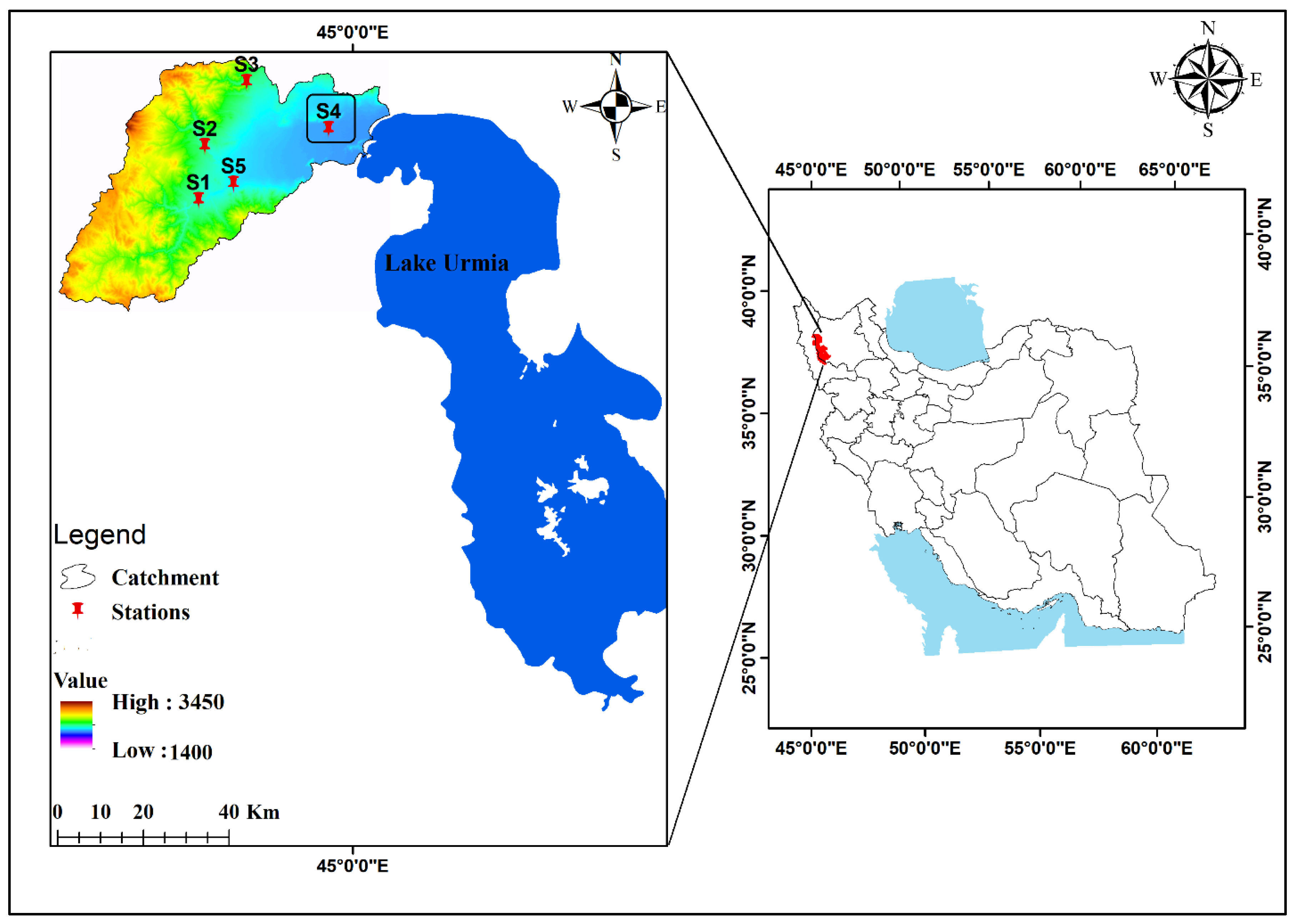
Figure 1. Zolachai River catchment area and location of Yalghouz Aghaj hydrometric station.
Water 16 02818 g001
Figure 2. Flowchart of present study methodology.
Water 16 02818 g002
Figure 3. The time series of input parameters (a) TDS, (b) Cl, (c) temperature, and (d) total hardness in the period of 1975–2016.
Water 16 02818 g003
Figure 4. A simple structure of the ANN [15].
Water 16 02818 g004
Figure 5. A typical arrangement of BRT [45].
Water 16 02818 g005
Figure 6. ELM structure [52].
Water 16 02818 g006
Figure 7. Social structure of grey wolves [54].
Water 16 02818 g007
Figure 8. Modeled TDS in training and testing stages using ML models (a) ANN, (b) GPR, (c) SVM, (d) LR, (e) CART, (f) BRT, and (g) GWO-KELM.
Water 16 02818 g008
Figure 9. Violin plot to compare the efficiency of machine learning models in TDS modeling.
Water 16 02818 g009
Table 1. Statistical summary of input parameters for TDS modeling.
ParametersNMeanMedianStd. Error of MeanMinMaxStd. Deviation
TDS (mg/L)504510.83409.0015.02166.002752.00337.31
Cl (mg/L)5042.000.870.150.2027.403.36
TH5042.972.730.051.1510.101.10
Temperature (°C)50417.6517.740.450.0034.7010.05
Table 2. Modeled TDS in training and testing stages using different ML models.
Model TypeMAE
(Training)
RMSE
(Training)
R2
(Training)
MAE
(Testing)
RMSE
(Testing)
R2
(Testing)
GWO-KELM40.7358.690.97234.4055.750.974
ANN40.27557.460.97138.2560.130.969
GPR36.2652.980.97640.7465.380.962
SVM40.7755.750.97242.9769.560.959
LR41.65757.310.97144.3274.180.953
CART55.36194.550.92456.498102.0640.908
BRT51.37686.6330.93653.828108.9390.895
Table 3. Comparing the accuracy of TDS modeling with previous works.
ReferenceMethodInput ParametersBest Model
Al-Mukhtar and AL-Yaseen, 2019 [15]ANFIS, ANN, MLRNO3, Ca+2, Mg+2, TH, SO4, ClANFIS: 0.97
Banadkooki et al., 2020 [9]ANFIS, SVM, ANNNa, Mg, Ca, HCO3, SO4, Cl ANFIS-MFO: 0.94
Ewusi et al., 2021 [16]GPR, BPNN, PCRAs, Cd, Hg, Cu, CN, TSS, pH, Turbidity, ECGPR: 0.99
Adjovu et al., 2023 [21]SVM, LR, KNN, ANN, GBM, RF, ET, XGBoostEC, TemperatureLR: 0.82
Hijji et al., 2023 [19]ANN, ELM, ANFIS, NF-GMDH-GOA NF, GMDH-PSO, GMDHNa, Mg, Ca, HCO3NF-GMDH-GOA: 0.97
Pourhosseini et al., 2023 [18]SVM-CA, SVM-HS, SVM-TLBONa, Mg, Ca, HCO3, SO4, Cl, pHSVM-TLBO: 0.99
Panahi et al., 2023 [17]ANN-CSA, ELM-CSANa, Mg, Ca, K, HCO3, SO4, Cl, pHELM-CSA: 0.97
This studyGWO-KELM, ANN, GPR, SVM, LR, CART, BRTCl, TH, TemperatureGWO-KELM: 0.974
Disclaimer/Publisher’s Note: The statements, opinions and data contained in all publications are solely those of the individual author(s) and contributor(s) and not of MDPI and/or the editor(s). MDPI and/or the editor(s) disclaim responsibility for any injury to people or property resulting from any ideas, methods, instructions or products referred to in the content.