Article

Water Inflow Forecasting Based on Visual MODFLOW and GS-SARIMA-LSTM Methods

College of Geoscience and Surveying Engineering, China University of Mining & Technology, Beijing 100083, China
*
Author to whom correspondence should be addressed.
Water 2024, 16(19), 2749; https://doi.org/10.3390/w16192749
Submission received: 1 August 2024 / Revised: 23 September 2024 / Accepted: 24 September 2024 / Published: 27 September 2024

Abstract

:
Mine water inflow is a significant safety concern in coal mine operations. Accurately predicting the volume of mine water inflow is vital for ensuring mine safety and environmental protection. This study focused on the Laohutai mining area in Liaoning, China, to reduce the reliance on hydrogeological parameters in the mine water inflow prediction process. An integrated approach combining grid search (GS) with the Seasonal Autoregressive Integrated Moving Average (SARIMA) and Long Short-Term Memory (LSTM) model was proposed, and its results were compared with Visual MODFLOW. The grid search was used to optimize the SARIMA model, modeling the linear component of nine years of water inflow data, with the remaining six months of data used for model validation. Subsequently, the prediction residuals from the SARIMA model were input into the LSTM model to capture the nonlinear features in the data and enhance the generalization capability and stability of the LSTM model by introducing Dropout, EarlyStopping, and the Adam optimizer. This model effectively handles long-term trends and seasonal fluctuations in the data while overcoming limitations in capturing periodicity and trends in complex time series data. The results indicated that the GC-SARIMA-LSTM model performs better than the Visual MODFLOW numerical simulation software in predicting mine water inflow. Therefore, without hydrogeological parameters, the GC-SARIMA-LSTM model can serve as an effective tool for short-term prediction, advancing the application of deep learning in coal mine water inflow forecasting and providing reliable technical support for mine water hazard prevention.

1. Introduction

China is the largest coal producer in the world, accounting for nearly half of the global coal production [1]. Coal remains a dominant force in China’s energy structure, and the development and utilization of coal resources are essential for the growth of the national economy [2]. Due to the complex geological, tectonic, and hydrogeological conditions, mine water disaster is a significant hazard that significantly impacts the safe extraction of coal resources. According to the statistics, issues related to mine water disasters in coal mines are second only to gas explosions in terms of significant disasters. Moreover, coal mine water disasters often result in severe casualties [3,4], challenges in rescue and relief efforts, and prolonged restoration of mining operations [5]. Accordingly, throughout the extensive process of mining coal resources, China has actively developed theories, technologies, and support systems for preventing and controlling mine water disaster in coal mines [6]. Despite advancements, further exploration into theories and practical technologies for controlling mine water disaster remains critical [7,8].
Owing to China’s complex geological and hydrogeological conditions, obtaining relevant hydrogeological parameters is challenging. Although predicting mine water inflow is crucial in exploration and production, research remains inadequate. Currently, traditional methods for predicting mine water inflow include hydrogeological simulation [9], analytical methods [10], numerical simulation [11,12], and time series methods [13,14,15,16]. Numerical simulation software primarily includes GMS 10.0 [17], FLAC 3D 6.0 [18,19], and Visual MODFLOW 4.2 [19,20,21,22,23]. However, these traditional methods depend on complex geological data to define boundary conditions [24,25]. Acquiring this geological data presents a significant challenge. Additionally, certain geological conditions may change with ongoing mining operations, increasing the difficulty in data acquisition and reducing data availability, further impacting the models’ accuracy [26]. The hydrogeological simulation method is easy to apply and straightforward but yields coarse prediction results. The analytical method is widely used and simple to calculate, yet determining the boundary conditions and calculation parameters is challenging. The numerical simulation method is commonly used to address complex boundary conditions and offers fast and precise results, but it requires highly accurate aquifer hydraulic parameters.
In recent years, time series analysis has played an essential role in geology, hydrology, water resources, and the environment [27]. Weiß highlights the advancements in time series modeling, illustrating its crucial role in handling data sequenced through time. This field encompasses a broad range of applications from stochastic processes, forecasting, and model fitting to diagnostics, leveraging both traditional statistical methods and machine learning techniques for enhanced analytical precision and forecasting accuracy [28]. Yu et al. utilized a BP neural network to effectively predict the depth of floor destruction caused by underground mining pressure, enhancing safety measures against potential water inflow from aquifers [29]. Choubin et al. developed combined gamma and M-test-based ANN and ARIMA models to forecast groundwater level fluctuations in semiarid regions, enhancing the accuracy of predictions through optimized input selection and training data length [30]. Valipour utilized SARIMA models to effectively forecast long-term runoff in the United States, demonstrating that SARIMA models, incorporating seasonal patterns, provide higher accuracy than traditional ARIMA models, especially when applying appropriate periodic terms [31]. Bouzghiba et al. enhanced short-term predictions of PM10 and NO2 concentrations in urban environments using the ARIMA search grid modeling, optimizing model parameters with Akaike and Bayesian information criteria to improve air quality management [32]. Gao and Hou enhanced the efficiency and accuracy of fault diagnosis in industrial processes by integrating a grid search-optimized Support Vector Machine (SVM) with Principal Component Analysis (PCA), demonstrating superior performance in the classification of system statuses under various operational conditions [33]. A prediction model based on the LSTM was proposed by Yan et al. to forecast the influx trend, achieving better prediction results than the BP model [34]. Kong et al. employed computer vision and Long Short-Term Memory techniques to predict unsafe behavior in construction environments, significantly improving safety management by integrating SiamMask for real-time tracking and an enhanced Social-LSTM model for dynamic behavior prediction [35]. Emami et al. significantly advanced the optimization of multi-reservoir systems by combining the strengths of ARIMA and LSTM models and employing a grid search to fine-tune model parameters, thereby improving prediction accuracy and operational efficiency [36]. Ji et al. introduced an innovative forecasting model, the ARIMA-CNN-LSTM, to predict carbon futures prices [37]. This model integrates the ARIMA model with deep learning techniques, specifically the Convolutional Neural Network (CNN) and the Long Short-Term Memory network, to enhance prediction accuracy by capturing both linear and nonlinear aspects of the data.
Research methods typically employ a single approach to predict water inflow without comparing traditional and machine learning methods. In this research, relevant parameters were first obtained from the results of pumping tests in the mining area, and Visual MODFLOW was used to simulate monthly water inflow for the next six months. Visual MODFLOW was selected for its lower computational demand and higher efficiency than GMS or FLAC 3D and its compatibility with AutoCAD 2018 to obtain more precise coordinates, elevation, and working range to establish a 3D groundwater flow model. Secondly, grid search (GS) will be used to optimize the hyperparameters of the SARIMA and LSTM models and predict the water inflow of the Laohutai mining area for six months in 2023. The optimization algorithms of two methods, SARIMA and LSTM, were then utilized to predict water inflow for six months in 2023 in the Laohutai mining area. The results from these methods were compared and analyzed to ensure the accuracy of predictions, aiming to achieve values close to actual data. The prediction results from numerical simulations, which utilize aquifer hydraulic parameters, were compared with time series model predictions based only on previously recorded influx data. It was concluded that short-term prediction results from GS-SARIMA-LSTM provide a solid theoretical basis for preventing sudden influx accidents in mine production, especially when various parameters are unavailable during actual production.

2. Materials and Methods

2.1. Study Area

The study area is situated in the intermountain alluvial valley north of the LaoXi Mountain—Laohutai—Wanxin Mountain hills and south of the Hun River within Fushun City, Liaoning Province, China (Figure 1). An erosional-accumulative terrain with a geomorphic pattern of dendritic narrow valleys characterizes the area. The hilly region consists of tuff and basalt. The overall terrain is higher in the south and lower in the north, with Laohutai Mountain, the southernmost peak, rising to 230.70 m. The central part of the coal mine area features a flat terrain that forms an alluvial plain, generally at an elevation of 80 to 100 m. To the north, the Hun River lies. Located in the middle temperate zone, the area experiences an average annual precipitation of 804.2 mm. The hydrogeological characteristics of this area include multiple layers of rock with varying permeability, which significantly impact hydrodynamics and mine safety. Recent studies have shown that groundwater flow characteristics directly influence mine safety, especially during extreme rainfall or significant fluctuations in groundwater levels [38]. The lithology of the aquifer and the recharge and discharge processes of groundwater play a critical role in mine safety management. These studies provide valuable references for mining areas with complex geological conditions, such as Fushun’s Laohutai, helping to predict and prevent mine water hazards and ensure safe mine management under complex geological structures and multilayer permeable rocks [39].
The structure of the study area is an asymmetric oblique tectonic with two flanks, which is slow in the south and steep in the north, and the south flank has a gentle dip. Most of the south side of the Laohutai surface was stripped by the East Open Pit Mine, and the north side is a subsidence backfill area. Three aquifers are mainly developed in the area: the alluvial sand and gravel aquifer, the marl aquifer, and the tuff basalt aquifer. Among them, the alluvial layer is located above the bedrock denudation surface, with a thickness of 4~24.3 m, and consists of sand pebbles with varying coarseness and fineness. The unit water inflow q = 4.12~0.841 L/(s·m), the permeability coefficient k = 8~20 (it is the principal aquifer); the marl aquifer layer is developed in the whole area, the vertical thickness is within 600 m, the unit water inflow q = 0.07 L/(s·m), the permeability coefficient k = 0.00065 (it is the overburden aquifer of the top of the coal seam of the production of the mine area); the thickness of the tuff basalt aquifer layer is 8~51.5 m, the unit water inflow q = 0.516~0.0000015l L/(s·m), and the permeability coefficient k = 1.178~0.000228. There are 11 significant faults in the mine area, primarily muddy debris, calcite filled, and closed fault, according to the pre-pumping test data. According to the data of the previous pumping test, the results of the mixed pumping test of F1 and gravel show that the unit water inflow of this fault is 0.000000199 L/(s·m) and the permeability coefficient is 0.00000256 m/d, and the pumping test of the faults of F1 and F1A shows that the unit water inflow is 0.00000012~0.0000247 L/(s·m). This indicates that the fault itself is weakly water-rich. Therefore, we do not focus on this paper’s faults and other structures.

2.2. Numerical Simulation Method

The mathematical concept of numerical simulation involves substituting a finite set of discrete points within the study area for a continuously varying infiltration area. This method replaces derivatives with difference quotient approximations at these discrete points. Consequently, partial differential equations and their boundary conditions are discretized into a finite number of algebraic equations for solving. This approach yields approximate values of groundwater levels at specific moments and discrete points within the infiltration area. A series of specific mathematical models are constructed by integrating mathematical expressions that reflect the specific geological conditions of the study area—namely, the boundaries and initial water levels. The outcomes from these mathematical models can then be translated into precise water flow models and predictions, where numerical simulation serves as the mechanism for solving the chosen mathematical formulations. In this paper, a three-dimensional seepage model was established using Visual MODFLOW 4.2. This software, developed by the U.S. Geological Survey for numerical groundwater simulation, employs three-dimensional finite-difference methods [40]. Given that hydrogeological parameters in the study area vary with lithology, the groundwater system is characterized as a non-homogeneous, anisotropic, three-dimensional, transient flow system suitably modelled using Visual MODFLOW. The aquifer under investigation is non-homogeneous and anisotropic, with the entire infiltration area experiencing three-dimensional unsteady movement. Based on Darcy’s law and the continuity equation for seepage, a corresponding three-dimensional transient flow mathematical model is established as follows:
x ( K x h x ) + y ( K y h y ) + z ( K z h z ) = S h t ,   ( x ,   y ,   z ) Ω
K x ( h x ) 2 + K y ( h y ) 2 + K z ( h z ) 2 h z ( K z ) = μ h t ,   ( x ,   y ,   z )   Γ 0
h ( x ,   y ,   z ) | t = 0   =   h 0 ( x ,   y ,   z )   ( x ,   y ,   z ) Ω
h(x, y, z, t)|Γ1 = h1(x, y, z, t) (x, y, z) ∈ Γ1
K n h n | Γ 2 = q ( x ,   y ,   z ,   t ) ,   ( x ,   y ,   z )   Γ 2
In the above equation: Ω is the permeable flow region; h is the groundwater level elevation, in meters; Kx, Ky, and Kz are the permeability coefficients in the x, y, and z directions, in m/d; Kn is the permeability coefficient in the direction average to the boundary interface, in m/d; S is the storativity of the aquifer below the free surface, in 1/m; μ is the gravity water supply degree of the confined aquifer; Γ0 is the upper boundary of the porous flow region; Γ1 and Γ2 are the first and second type boundaries of the porous flow region; q(x, y, z, t) is the defined unit area flow across the second type boundary of the aquifer, with inflow as positive, outflow as unfavorable, and zero for impervious boundaries, in m3/m2·d.
Considering the limited number of hydrological observation wells, interpolation was employed to enhance the data while constructing the numerical simulation model. Initially, spatial interpolation using Surfer 16 software was utilized to estimate the initial water levels. This approach offers a more continuous and comprehensive representation of initial hydrological conditions by statistically evaluating the water level distribution across the study area based on sparse data from available observation wells. Furthermore, due to the data constraints, zoning of permeability parameters was established based on the results from existing pumping tests. This zoning involves segmenting the study area according to groundwater flow and infiltration characteristics, with distinct permeability parameters potentially assigned to each segment. Such zoning facilitates more precise modeling of groundwater flow dynamics across different regions and provides a scientific foundation for water resource management and protection. While the number of data points constrains this method, the accuracy and practicality of the simulation can be significantly enhanced by applying robust mathematical models and computational methods.

2.3. Time Series Method

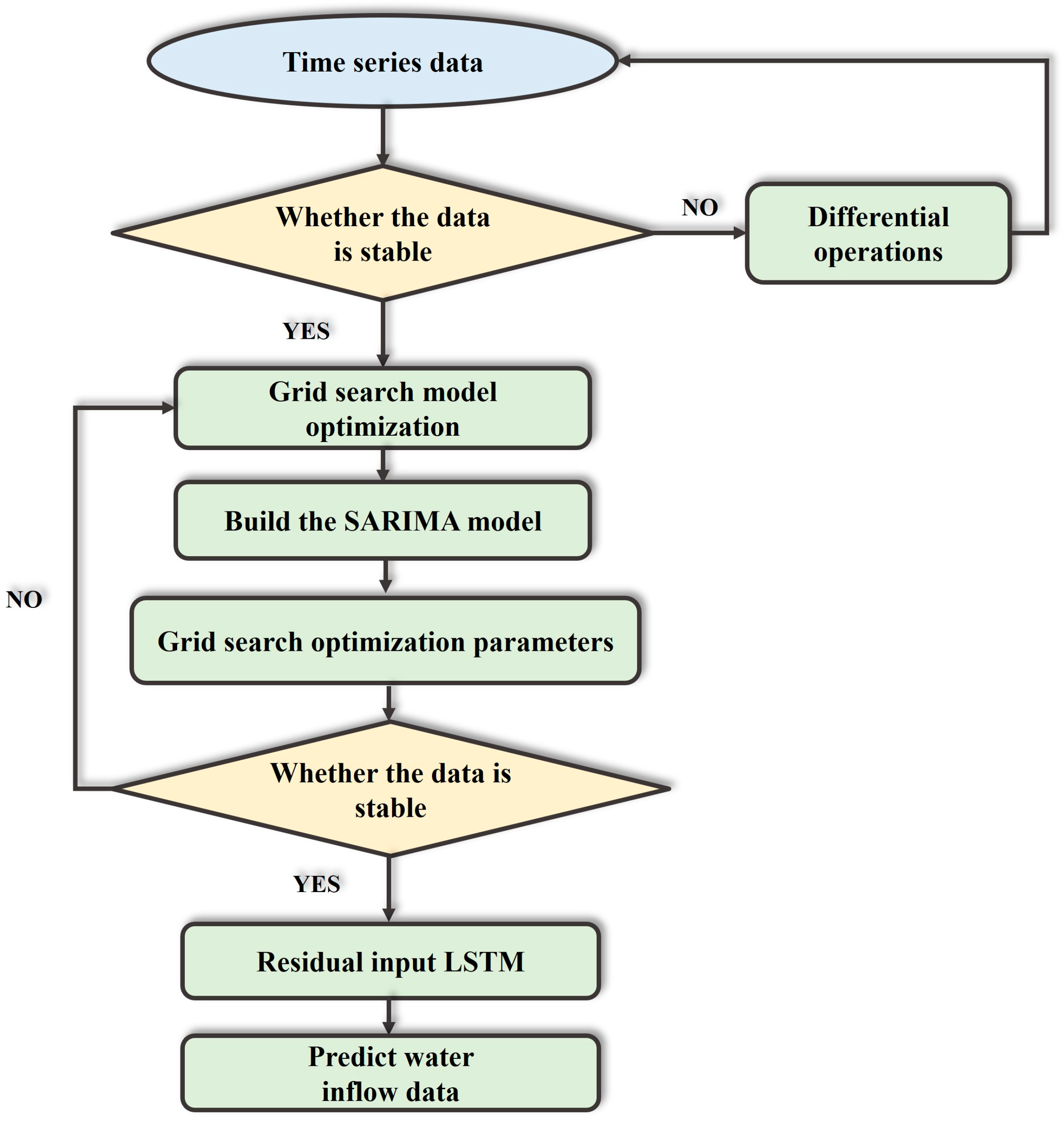
The construction of the GS-SARIMA-LSTM model primarily involves using the SARIMA model to address the linear relationships and seasonality in the time series. In contrast, the LSTM model captures the nonlinearity and long-term dependencies. Initially, the SARIMA model is applied to model the time series data. A grid search is then conducted to optimize the SARIMA parameters for improved prediction accuracy. Subsequently, the residuals from the SARIMA prediction results are used as inputs for the LSTM network. These residuals are then further modeled and predicted by the LSTM, effectively enhancing the model’s ability.
The SARIMA (Seasonal Autoregressive Integrated Moving Average) model is a prevalent statistical method for time series forecasting, particularly effective for non-stationary data [41]. It combines aspects of autoregression (AR), differencing (I) to achieve stationarity, and moving average (MA) components. SARIMA is denoted as (p, d, q)*(P, D, Q) [42].
AR is “autoregressive”, p is the number of autoregressive terms, MA is “sliding average”, q is the number of sliding average terms, and d is the number of differences (order) made to make it a smooth series; P, D, and Q are seasonal parameters added to the basic ARIMA model, which denote the seasonal autoregressive order, the seasonal difference order, and the seasonal moving average order, respectively.
AR is a model that indicates that the value of a variable at the current moment in time depends on, and only depends on, the value of a variable at several points in time in the past. It is called an autoregressive model because it does not depend on other explanatory variables. The parameter p denotes the number of recent historical values on which the model depends, denoted as the AR(p) model:
x t = μ + i = 1 p φ i x i 1 + ε t
where x t is the current value, μ is the constant term, p is the order, φ i is the autocorrelation coefficient, and ε t is the error, which is also white noise.
I model is a difference model that serves to smooth a time series. A standard method of converting an unsteady series into a smooth series is differencing.
d = y t y t 1
d y t = d 1 y t d 1 y t 1
Here, d denotes the order of differencing. The process of smoothing a time series may require more than one differencing.
The MA model, also called the moving average model, represents the dependence of the value at the current point in time on the value of the q most recent historical prediction error in the past. Here, q denotes the number of lags in the forecast error, also called the number of sliding average terms. The MA(q) model can be expressed as follows:
x t = μ + ε t + i = 1 q θ i ε i 1
where x t is the current value, μ is the constant term, q is the order, θ i is the autocorrelation coefficient, and ε t , ε i 1 is the error.
The parameters P, D, and Q in the SARIMA model are determined using the Autocorrelation Function (ACF) and the Partial Autocorrelation Function (PACF). The ACF provides insights into the correlation of the data at various time points within a series, capturing both direct and indirect correlation information. Conversely, the PACF helps identify the lag order in a time series by isolating the direct relationship between an observation and its lag, adjusting for influences from all shorter lag terms. It primarily assesses the correlation between the observation yt and its lag yt−i after removing the effects of intervening lags.
Although ACF and PACF plots are helpful for the initial selection of SARIMA parameters, experimenting with different combinations is crucial to pinpoint the optimal values for the SARIMA model parameters. This study used the grid search method to automate selecting the optimal SARIMA model parameters, determining the most effective combination for our modeling needs.
The Stationary test is used to determine whether the statistical properties of a time series remain constant over time. Stationarity is a critical property in time series analysis, as many time series models (such as SARIMA) assume the data is stationary.
A D F = γ ^ S E γ ^
where γ ^ is the estimated coefficient of the lagged term in the regression model, and S E γ ^ is its standard error. Based on the p -value of the test results, we determine whether to reject the null hypothesis.
If p > 0.05, the null hypothesis cannot be rejected, indicating the series is non-stationary, and differencing is required d 1 .
If p ≤ 0.05, the null hypothesis is rejected, indicating the series is stationary, and no differencing is required d = 0 .
Grid search with cross-validation is a comprehensive algorithm that maps all possible parameter values a model requires into a grid structure. This method systematically tests various combinations of parameter values to automatically identify the optimal set necessary for the model. This automatic parameter tuning process is supported by a scoring system provided by cross-validation. Commonly used cross-validation methods include 3-fold, 5-fold, and 10-fold cross-validation. These methods score each parameter combination based on their performance, and the algorithm ultimately selects the combination with the highest score for the modeling process. This approach ensures that the chosen parameters are the most effective for the given data and modeling objectives.
Residuals are used as the target variable for the LSTM model to capture the remaining nonlinear patterns.
r t = y t y ^ t , S A R I M A
where r t is the residual of the SARIMA model, which is used as the input to the LSTM model.
LSTM was co-proposed in 1997 as Long Short-Term Memory (LSTM) [43], a high-level recurrent network that uses memory blocks to model long-term dependencies. Memory blocks consist of storage cells and three special gates for remembering the temporal states of the network [44]. These three gates are the Input Gate, Output Gate, and Forget Gate. The LSTM model utilizes gating mechanisms to control the updating and resetting of hidden states. The Input Gate decides when information is to be read into the memory cell, the Output Gate decides whether information in the memory cell should be allowed to affect output at the current time, and the Forget Gate decides whether current data should be retained or discarded. Additionally, to address the issue that neural networks like traditional RNN models are sensitive to short-term inputs and not ideal for long-term memory, a Memory Cell is added inside LSTM models to enable long-term cyclic transfer of information. Using the Memory Cell and gating mechanism, the long-term dependence of the time series is effectively captured by the LSTM model. Therefore, the LSTM model is widely used in time series forecasting.
As the first step, the primary role of the Forget Gate is selecting which information to keep and which to forget by evaluating the importance of memorized information in the cell state of the previous moment at the current moment. The output ht−1 of the prior moment and the input xt of the current moment are transformed into a vector using a sigmoid function by the Forget Gate. Each element’s numerical magnitude in this vector represents the retention ratio of memorized information in the cellular state, with values ranging from 0 to 1 [35]. The specific formula is presented as follows:
f t = σ ( ω f h t 1 , x t + b f )
where f t is the oblivion gate, σ is the sigmoid activation function, and hidden is the unit state at the moment, h t 1 . The input to the x t is “input to the” oblivion gate, ω f is the coefficient of the linear relationship of the oblivion gate, and b f is the bias of the oblivion gate. f t varies between 0 and 1, and if f t = 0, all information about the previous state is ignored.
The Input Gate determines which information can be used to update the current memory cell state, utilizing the tanh function to control new information added to the network. The tanh function creates a new memory cell to hold this new information, according to Equations (9) and (10); the Sigmoid function is employed to determine usable information, followed by the Tanh function to generate a candidate memory cell state.
c t = tan h ( ω c h t 1 , x t + b c
i t = σ ω i h t 1 , x t + b i
where c t is the candidate memory cell state, ω c is the weight matrix of the Input Gate, b c is the bias term of the candidate memory cell, ω i is the weight matrix of the candidate memory cell, and b i is the bias term of the Input Gate.
When input information h t 1 , x t is processed by the Forget Gate and Output Gate, the cell state must be updated to form new long-term memory. Updating the formula is shown as follows:
c t = f t c t 1 + i t c t
where f t is the output of the Forget Gate, i t is the output of the Input Gate, and c t is the candidate memory cell state.
The Output Gate selectively outputs the cell state at the current moment; its calculation is divided into two parts: determining which input information the sigmoid function can produce and processing the already updated cell state using the tanh function. The product of these two processes forms the output. The specific calculation formula is as follows:
O t = σ ω a · h t 1 , x t + b a
h t = O t tan h c t
where ω a is the output weight matrix, O t is the Output Gate, and b a is the output bias term.
To prevent overfitting in the training process of the LSTM model, the Dropout regularization technique was introduced. During training, Dropout randomly drops some of the neurons in the network, forcing the network to learn more generalized features. The specific calculation formula is as follows:
y = 1 p · i = 1 n D i · w i · x i
where D i is an independent Bernoulli random variable that determines whether a neuron is retained, and p represents the probability of retention The model can avoid over-reliance on specific neurons by using Dropout, thereby enhancing its generalization ability.
EarlyStopping is a strategy to prevent overfitting by monitoring the model’s performance on the validation set. When the performance no longer improves, training is automatically stopped. The core idea is to use the validation set to determine when the model has reached its optimal state, thus avoiding overtraining and overfitting.
l o s s v a l t m i n l o s s v a l t k , k > 0
The Adam optimizer combines the concepts of Momentum and adaptive learning rate, making it a commonly used optimizer in gradient descent algorithms. It dynamically adjusts the learning rate by storing estimates of the first and second moments, thereby improving the model’s convergence speed and stability.
m 0 = 0 , v 0 = 0
g t = θ L θ t 1
m t = β 1 m t 1 + 1 β 1 g t
v t = β 2 v t 1 + 1 β 2 g t 2
m t ^ = m t 1 β 1 t , v t ^ = m t 1 β 1 t
θ t = θ t 1 α m t v t ^ + ϵ
where m t and v t represent the first and second moment estimates of the gradients, respectively, while β 1 , β 2 are the decay rates of the moments and α is the learning rate.
Time series models encompass both linear and nonlinear relationships, and the SARIMA model is a classical approach that primarily addresses linear relationships but yields suboptimal results for nonlinear data. The LSTM model accommodates both data types but does not consistently achieve uniform results across different datasets and struggles with comparative horizontal analysis. The hybrid model is updated to address linear and nonlinear data characteristics to optimize prediction outcomes. In time series analysis, the hybrid model effectively handles diverse data variations, delivering comprehensive results, superior analytical performance, and enhanced predictive accuracy. Hybrid models employ supervised machine learning algorithms to predict and train on diverse datasets and to improve model diversity. Results from hybrid models are more comprehensive than those from single models; despite imperfect data correlation, they significantly reduce variance and errors. Identifying a model that fits the data and proposing effective fusion strategies are crucial for addressing complex datasets. This paper utilizes the residuals of the SARIMA model as inputs to the LSTM model. Subsequently, the LSTM model output is calculated using the ARIMA model residuals. The outputs from both the LSTM and SARIMA models are then aggregated to derive the final output of the hybrid model.
â t = f r t 1 , r ( t p
o t = â t + o t a r i m a
where â t is the residual value output from the SARIMA model, which is incorporated into the hybrid LSTM mode; o t a r i m a indicates the value predicted by the SARIMA model. An advantage of this approach is the facilitated information exchange between the SARIMA and LSTM models. Below is the specific simulation flowchart (Figure 2):
Model performance is evaluated using root mean square error (RMSE) and R2 as metric [45], as specified in the following equation:
R M S E = i = 1 N y i x i 2 N
where N is the number of data points, y i is the ith actual value, and x i is the ith predicted value.
R 2 = 1 i = 1 n y i x i 2 i = 1 n y i y 2
where y i is the ith actual value, x i is the ith predicted value, and y is the average of exact values.

3. Results

3.1. Numerical Simulation Predicting

This study’s data collection site is the Laohutai mining area in Fushun, Liaoning Province, China. This area has complex hydrogeological conditions, with three significant aquifers: the alluvial sand and gravel aquifer, the marl aquifer, and the tuff-basalt aquifer. To ensure the comprehensiveness and representativeness of the data, continuous monitoring of mine water inflow in this area was conducted from January 2012 to June 2023, with monthly hydrological data collected. High-precision sensors were used for real-time monitoring during the data collection process, and the equipment was regularly calibrated to eliminate measurement errors caused by sensor drift. Standardized statistical methods, such as outlier removal and imputation techniques, were applied to handle outliers and missing values, ensuring the accuracy and consistency of the data. Additionally, multiple measurements and independent verifications were conducted to ensure the reliability of the data. Figure 3 below presents a hydrogeological generalization of the study area.
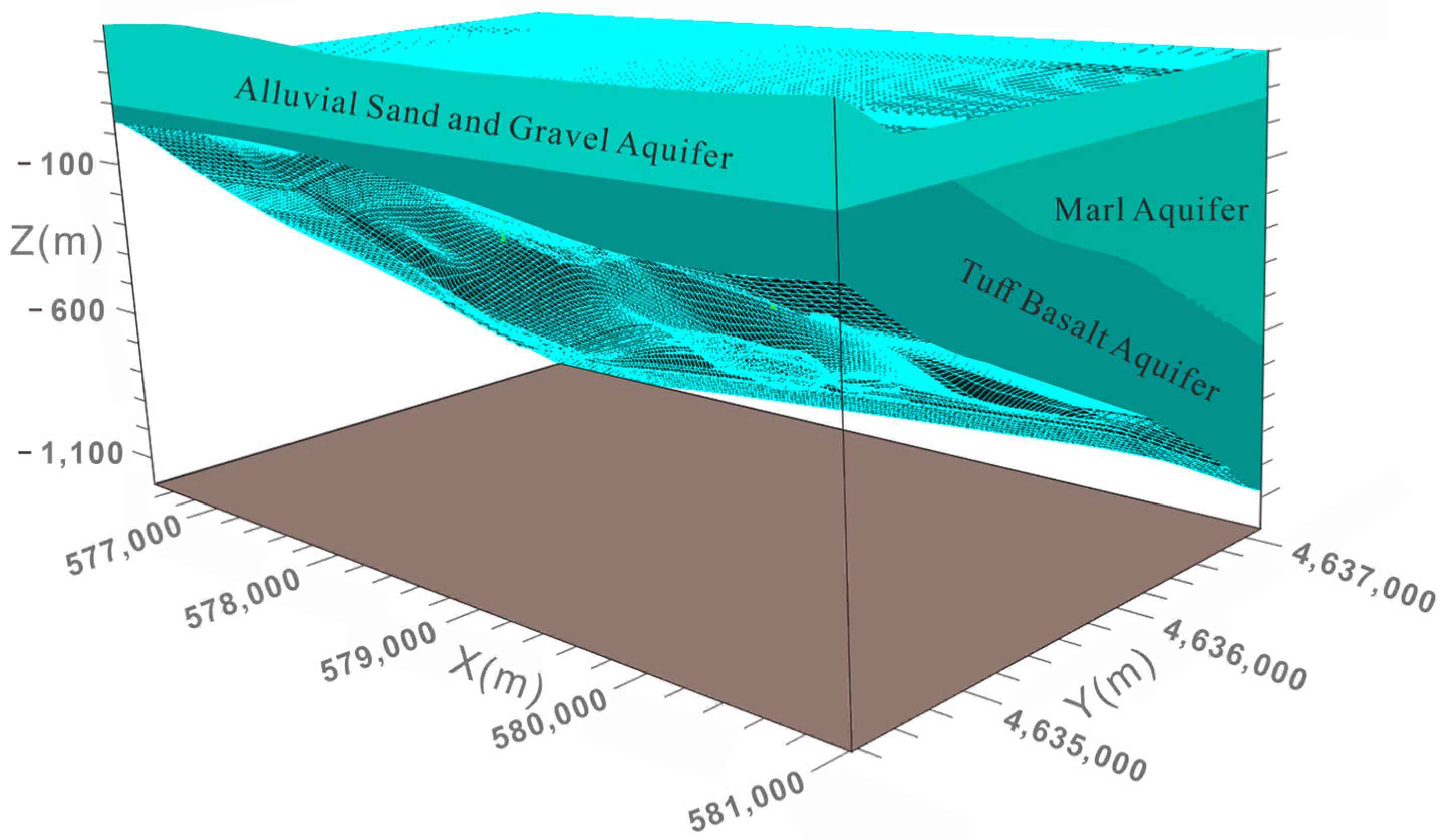
The elevation data for each layer point were derived from borehole test results, with elevation distribution for each aquifer roof elevation extended using the Kriging interpolation method. Flow model simulations under transient conditions were conducted over two months, from January to February 2023. The simulation area was delineated based on the minefield management area and partitioned into several grids, each grid cell measuring 80 × 80 m. Grids outside the mine were designated inactive, while only those within were subdivided. Hun River in the northern mining area, lacking direct hydraulic connection to the underground aquifer, was designated a fixed head boundary. The western boundary, covering Old West Mountain and Shengli Mining Area, was classified as water-isolated due to no direct hydraulic connection with the study area. Similarly, the southern boundary by Laohutai, the eastern boundary by Longfeng Jingtian, and the mining area, all lacking direct hydraulic connections, were designated as water-isolated boundaries. The first aquifer in study area, a submerged boundary, receives minimal atmospheric precipitation recharge and participates in cycle of evapotranspiration rate and excretion. Its surface maintains the direct hydraulic connection, while the model bottom comprises relatively watertight bedrock, designated as a watertight boundary. The three-dimensional geological model is established as follows Figure 4:
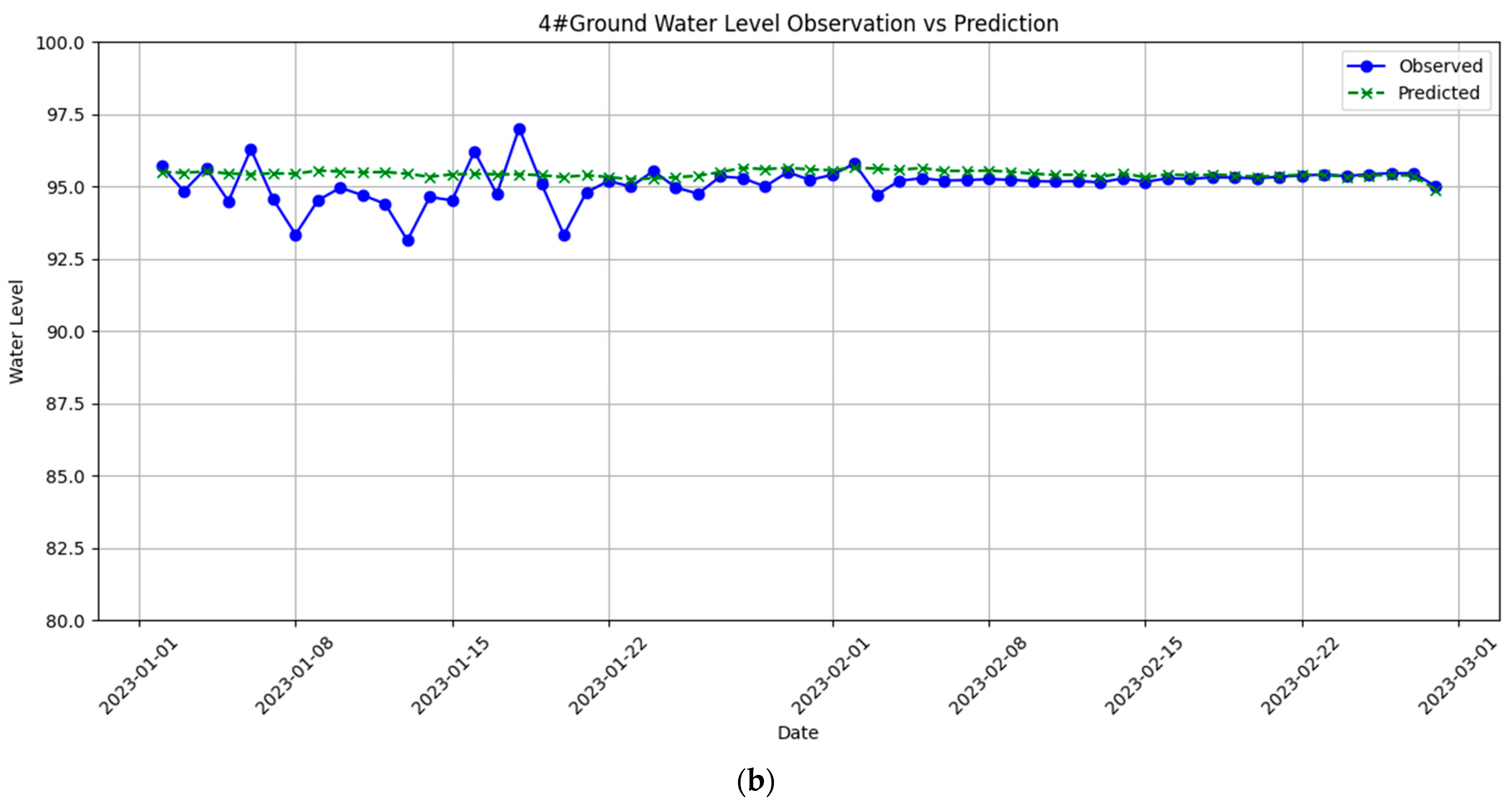
Before applying the numerical model to predict mine influx, verifying that the model aligns with the actual groundwater seepage system is crucial. Existing pumping test data from the study area aligned with the numerical predictions, verifying the model’s accuracy. A comparison will be made between the quaternary aquifer’s simulated groundwater head and the observation wells’ groundwater head. The measured and simulated water level values from hydrologic observation wells No. 2 and No. 4 for January to February 2023 are compared with their respective simulated values. Figure 5 presents the adjusted simulation results that correspond closely with the observation results.
The adjusted aquifer has been segmented into hydraulic conductivity zones, as depicted in Figure 6. The hydrogeological parameters for each aquifer are specified in Table 1.
Coal production is mainly located in the northern part of the mine area. Based on the distribution of the area and the mining plan, changes in water levels are predicted within two years of mining. As the mine area expands, dredging will be required to mitigate the risk of water surges. Due to inadequate groundwater recharge, mining and dredging will disrupt natural groundwater recharge, causing an imbalance in discharge and a subsequent decline in water levels in the northern area of the mine. As shown in Figure 7, the water level gradually declined over two years. Maintaining a continuous production plan may lead to a reduction in available groundwater resources, requiring protective measures.
Water inflow calculation in the study area primarily involves computing the aquifer water balance to determine the equivalent water inflow, specifically, by calculating the difference between the inflow and outflow of an aquifer at a specific moment. The visual MODFLOW zone equilibrium program is primarily used to process MODFLOW output data and compute the water balance in the study area. The model incorporates a zone budget module to facilitate water inflow calculations in specified areas. The results (Figure 8) illustrate the monthly water inflow for June 2023, with zones A, M, and T representing the water inflow into each aquifer and their aggregate representing the total water inflow for the mining area. The simulation results show that the groundwater head in the study area gradually decreases over time, particularly in the northern mining area, where a significant drop in water levels reflects the continuous depletion of groundwater resources. This trend is especially pronounced over the two-year simulation period, and the extent of the head decline is closely related to mining intensity and insufficient groundwater recharge. As the mining area expanded, the groundwater head reached an average daily inflow of 16,994 m3/d by June 2023, equivalent to 708.08 m3/h. Although numerical simulations can provide a three-dimensional dynamic representation of the groundwater system, the accuracy of the results heavily depends on the completeness of hydrogeological parameters and the correct setting of boundary conditions. The results are shown in Figure 8. Figure 8 presents the water inflow data under reduced, increased, and regular fits of permeability coefficients while keeping other parameters constant. The analysis reveals that the permeability coefficient has a significant impact on the sensitivity of the model. In actual mining operations, obtaining precise hydrological data becomes more challenging as geological conditions change, leading to more significant errors in the simulation predictions under certain circumstances. However, the advantage of numerical simulation lies in its ability to provide reliable long-term forecasts of future groundwater dynamics when sufficient hydrogeological data are available, making it an essential tool for mine hydrological forecasting when hydrogeological parameters are complete.

3.2. Time Series Predicting

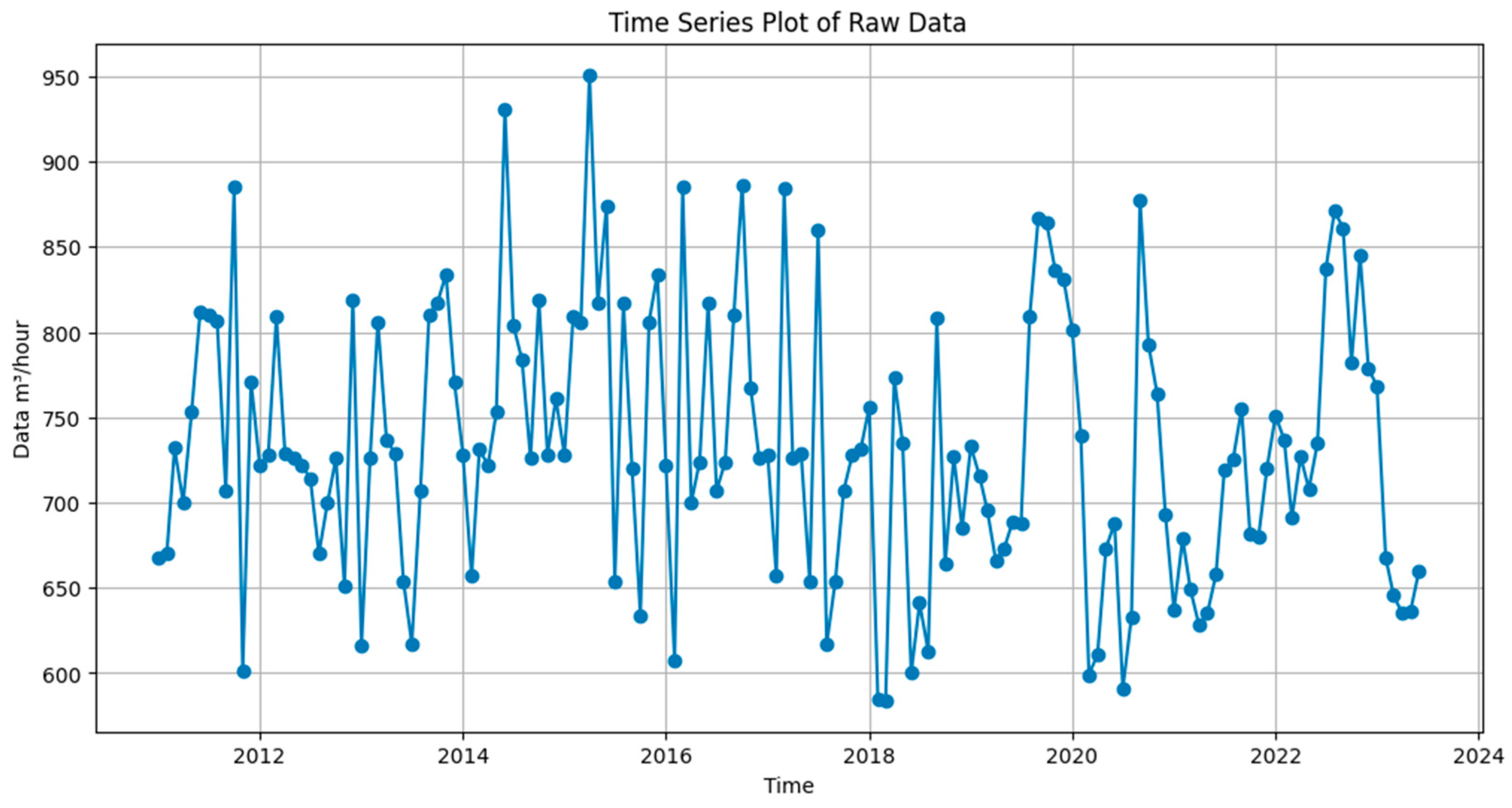
Monthly influxes from January 2012 to June 2023 were utilized as raw data in this study, as depicted in Figure 9.
The raw data are tested for smoothness to determine if differencing is necessary. Parameters such as the p-value and t-value from the ADF test on the raw series are examined in the table below, confirming the series is stationary and no differencing is required. Subsequently, white noise testing is performed, and with a p-value of 1.0286350206734886 × 10⁻¹⁴ being below the significance level of 0.05, the hypothesis of white noise is rejected. Consequently, the absence of white noise in the converted time series indicates that it is suitable for modeling and prediction. When the time series is converted to a steady-state data set, the difference order is 0, indicating that the hyperparameter d equals 0.
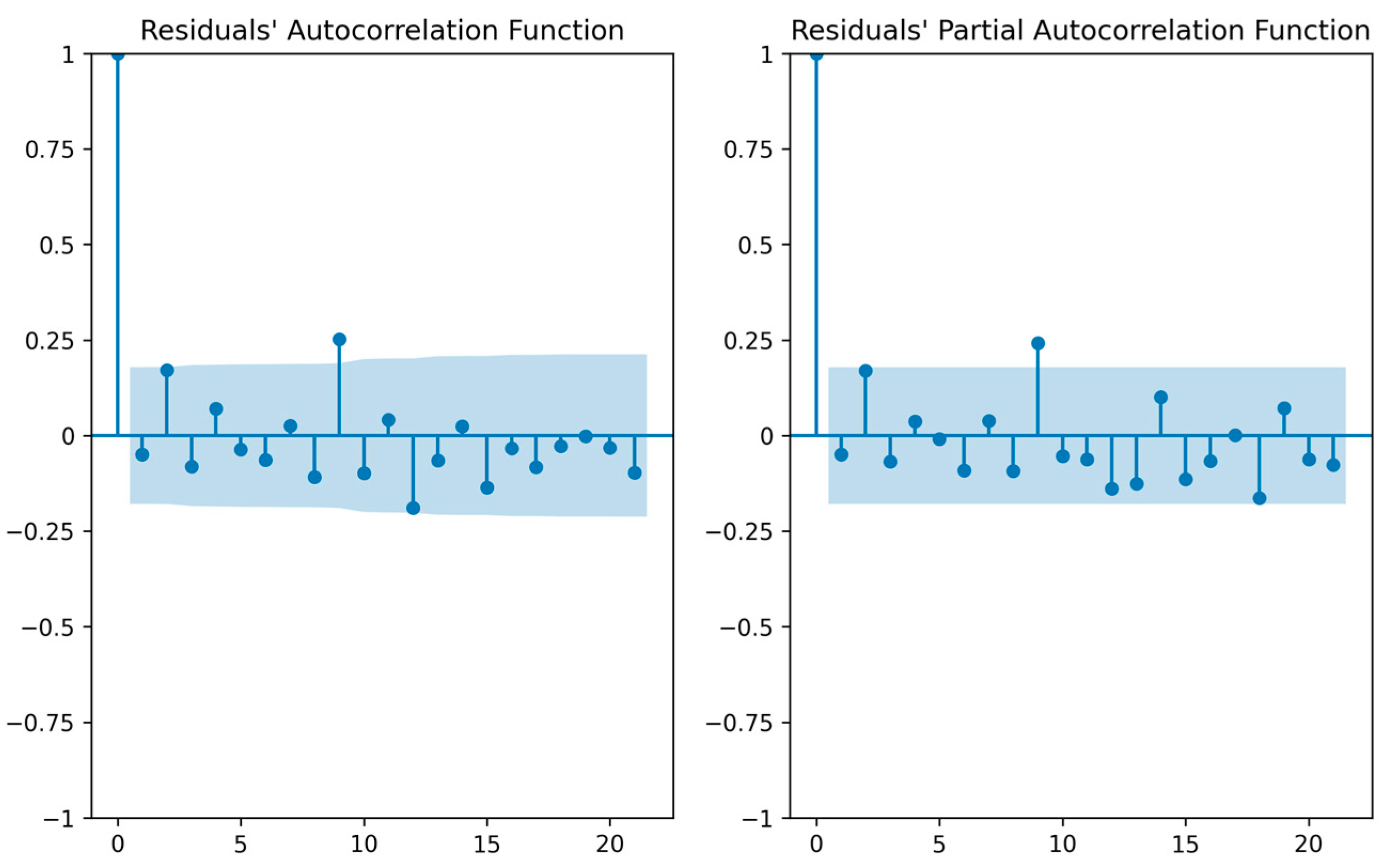
Hyperparameters p and q were determined using PACF and ACF plots, as illustrated in Figure 10. Blue bars represent significance confidence bands, within which the function value is considered zero. At lag 10, the ACF plot shows a significant non-zero value but does not truncate significantly within the lag period, suggesting a slight autocorrelation in the process. The PACF plot, displaying significant non-zero values at lag 10 and some lower order lags, does not truncate significantly within the lag period, indicating the absence of a significant AR process.
The optimal SARIMA model is identified by systematically evaluating various parameter combinations through grid search optimization, based on information criteria such as AIC and BIC. All SARIMA parameter permutations are listed to form a grid, with SARIMA modeling subsequently conducted based on these combinations. A scoring mechanism, such as cross-validation approach, is required to evaluate each model, with the highest scoring parameter combination ultimately selected as follows: Selected model parameters, SARIMA (0,1,1) (1,1,1) [12], are exhibited to perform best according to AIC and BIC values, indicating a good fit with data. The accompanying Figure 11 compares prediction results using a scatter plot.
The most suitable SARIMA training data length was determined for deriving the prediction results, and various segmentation length datasets were compared and segmented as depicted in Figure 12 and tables to identify the optimal segmentation lengths.
The RMSE was calculated based on the prediction results of different segmentation lengths. As shown in Table 2, the optimal segmentation length is when the training data are 80% of the original data.
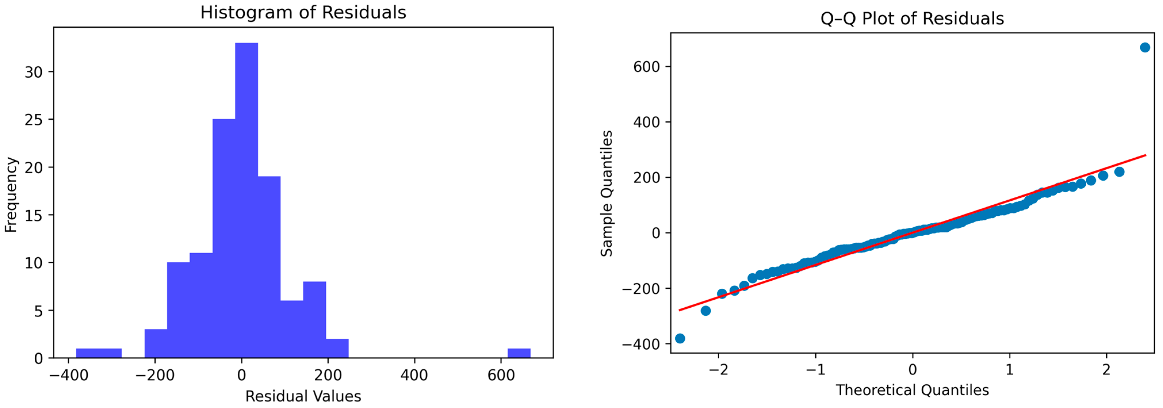
The SARIMA model results are primarily evaluated using residual tests. If residuals (residuals = actual observations − model predictions) are normally distributed, it can be inferred that they are stochastic, suggesting a better fit to the random error, as depicted in the figure. The normal distribution of residuals can be confirmed through the Q–Q plot, as illustrated in Figure 13. The Q–Q plot of residuals tests whether the residuals follow a normal distribution. The red line represents the theoretical quantiles under the standard distribution assumption. The residuals are approximately normally distributed if the residual points are distributed near this red line. The plot shows that most of the data points align closely with the red line, suggesting that the residuals largely conform to normality.
The prediction results on the test data exhibit high accuracy, verifying the validity and reliability of the time series model in practical applications. These results demonstrate that the GS-SARIMA-LSTM model performs well with time series data, utilizing both the SARIMA model’s ability to capture short-term fluctuations and the LSTM model’s strengths in handling complex and nonlinear trends, thereby offering an effective forecasting method for practical applications.
The results of Figure 14 indicate that, following optimization via grid search, the predictions (represented by blue dots) align more closely with the actual values.

4. Discussion

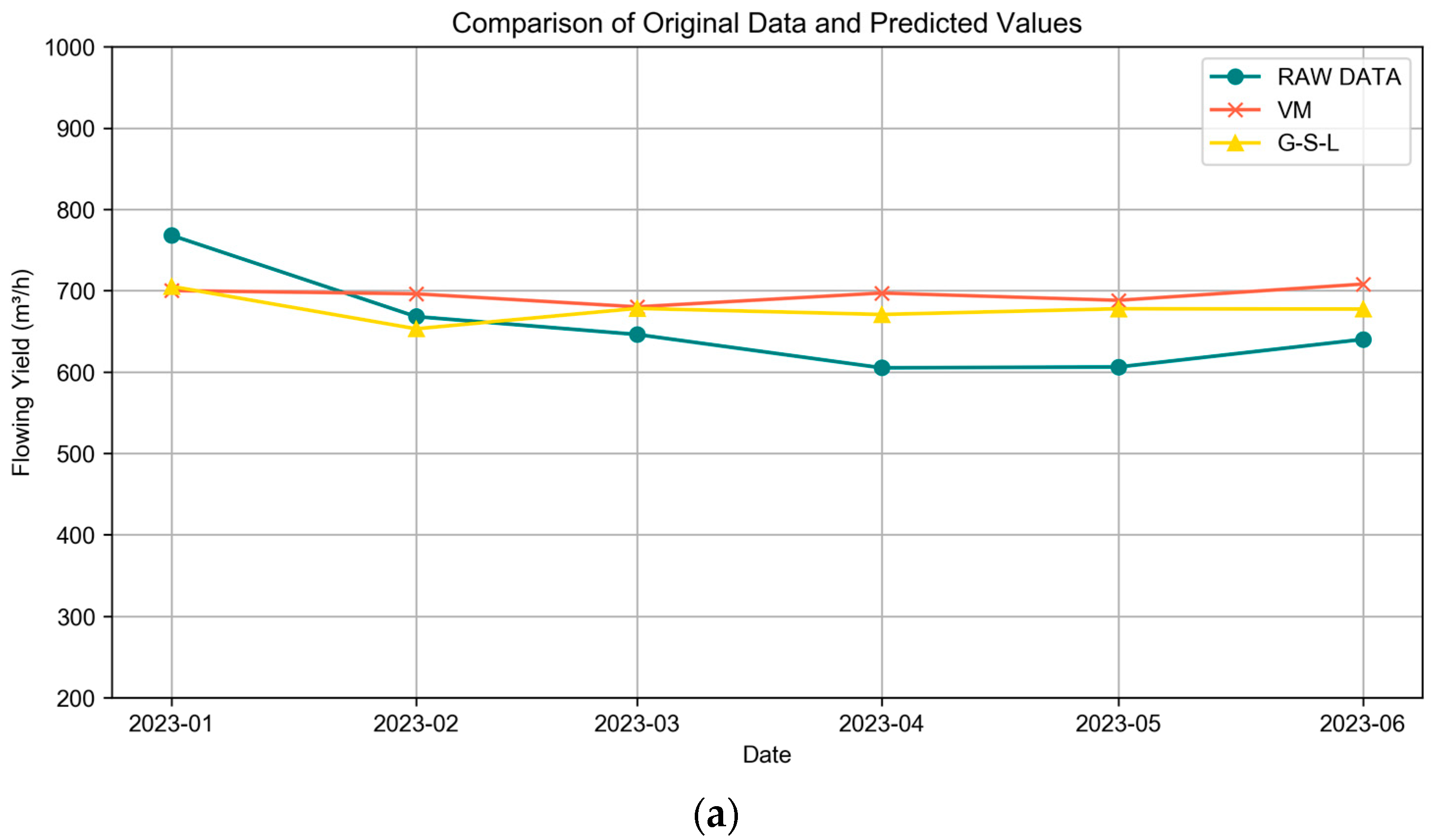
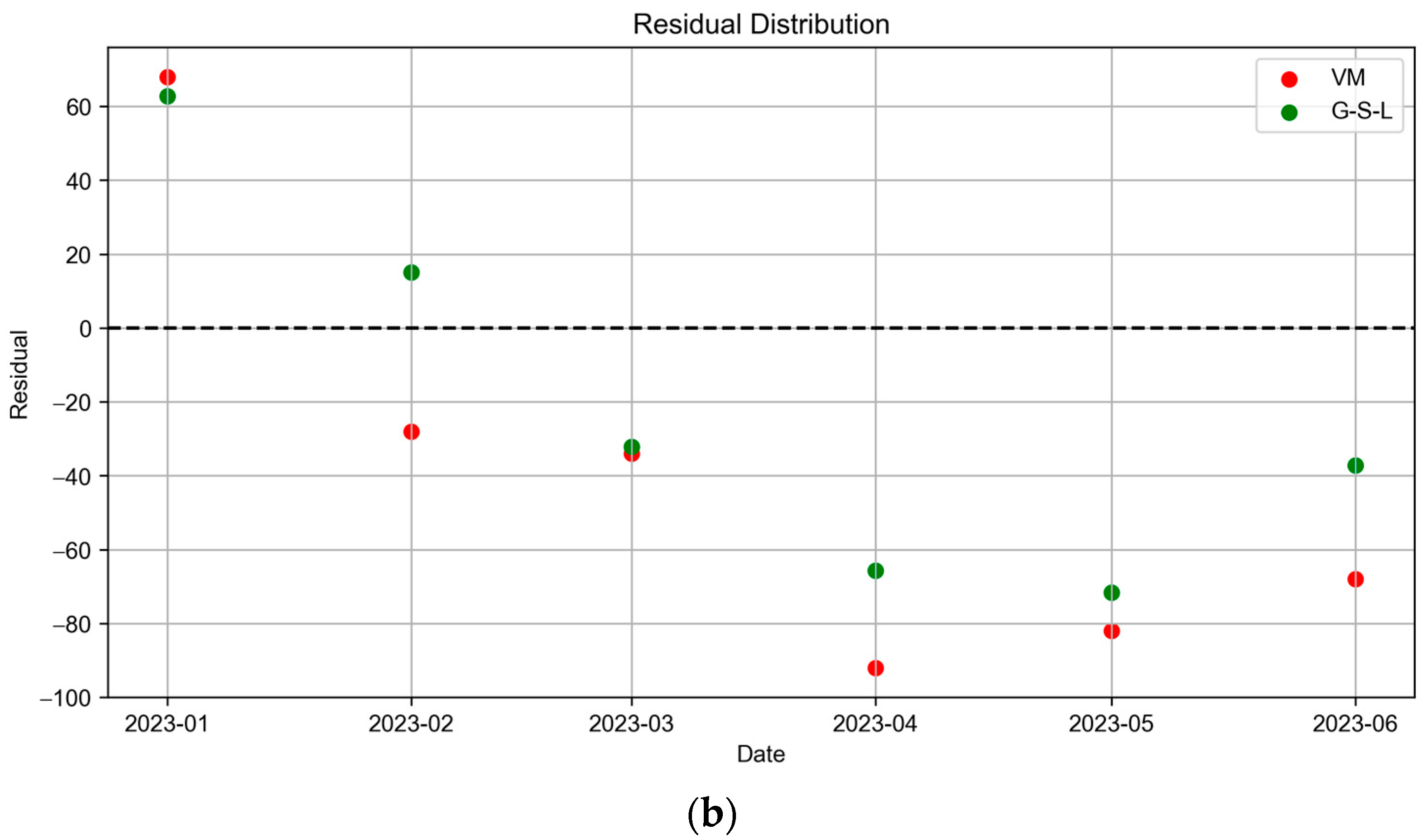
In this study, Visual MODFLOW was first selected for the numerical simulation of mine water inflow. Visual MODFLOW is one of the most widely used tools for groundwater flow simulation, suitable for heterogeneous anisotropic three-dimensional transient flow systems. When building the model, we conducted a detailed hydrogeological parameter zoning (such as permeability coefficients) of the study area to ensure the model’s accuracy and realism. Compared to other simulation tools, such as GMS and FLAC 3D, Visual MODFLOW has a higher computational efficiency and is easier to integrate with AutoCAD to obtain accurate three-dimensional coordinate data [46]. However, traditional numerical simulation methods often rely on complex hydrogeological data and require precise boundary condition settings, which introduces limitations in practical applications [47]. Therefore, we applied a GS-SARIMA-LSTM-based time series forecasting method to address the prediction challenges in cases where hydrogeological parameters are incomplete. To clearly demonstrate the effects of various prediction methods, a comparison chart of prediction trends is provided, as illustrated in Figure 15, thus demonstrating G-S-L’s slightly superior overall predictive effectiveness compared to VM. In monthly RMSE calculations, G-S-L consistently exhibits smaller errors than VM at all data points in Table 3. Particularly in April, May, and June, G-S-L RMSE values are significantly lower than those of VM, indicating G-S-L has a greater accuracy in these months, thereby confirming the method’s stability and precision in month-to-month predictions. R2 analysis indicates that an R2 value close to 1 signifies effective prediction and explanation of data variations. R2 comparisons show that G-S-L achieves positive R2 values in February, March, and June, with particularly high values in February and March, notably, 0.925511 in February, demonstrating exceptional model performance. Conversely, VM exhibits negative R2 values in most months, performing better only in February and March, yet still failing to surpass G-S-L performance.
Visualization and analysis of the residual plot and fitted curve graph reveal that G-S-L residuals are closer to the zero line and exhibit a more concentrated distribution, indicating smaller and more uniform prediction errors. Concurrently, G-S-L prediction curves align more closely with the raw data, demonstrating its enhanced capability in trend prediction. Specifically, in the residual plot, the G-S-L residual line (green) is closer to the zero line compared to VM (red), and features a more concentrated distribution, suggesting that G-S-L prediction errors are smaller and more uniformly distributed near the raw data. Regarding the fitted curve plots, G-S-L prediction curves better match the raw data, affirming its superior performance in capturing data trends and changes, particularly in upward and downward movements. G-S-L more accurately reflects the actual conditions, while VM exhibits some bias.
Time series prediction scenario methods have been increasingly applied to predict influxes [48,49]. SARIMA’s main approach involves adapting the model to seasonal variations through seasonal differencing, enhancing its ability to predict seasonal fluctuations in the data. However, SARIMA, which performs linear modeling, struggles with complex nonlinear problems [31,50,51]. LSTM, a widely utilized recurrent neural network, efficiently processes and memorizes long-term dependent information through its gating mechanism. It is noted for its simplicity and ease of training [52,53,54,55]. GS-SARIMA-LSTM merges SARIMA’s seasonal processing capabilities with LSTM’s long-term memorization abilities, enabling the effective handling of complex time series data with seasonal and long-term trends. An advantage of grid search is its systematic exploration of different parameter combinations to identify optimal settings for the model. By leveraging both GS-SARIMA-LSTM and grid search optimization, the model achieves greater accuracy and stability in handling complex time series data. This study compares the prediction capabilities of traditional Visual MODFLOW software and the GS-SARIMA-LSTM model by analyzing inflow data from January to June 2023. The study results indicate that G-S-L predictions more closely align with the raw data. G-S-L’s integration of time series analysis and deep learning enables it to more effectively capture dynamic changes and complex nonlinear relationships in the data, enhancing its surge prediction performance. Although G-S-L performed well in this study, its complexity and the high volume of data required may restrict its broader application. Future research could optimize G-S-L’s parameter settings and test it across diverse datasets to confirm its broad applicability and reliability.

5. Conclusions

This study analyzed Visual MODFLOW and the GS-SARIMA-LSTM model to compare water inflow predictions and to develop an efficient method for forecasting future inflow. The GS-SARIMA-LSTM model significantly improves prediction accuracy compared to traditional numerical simulation models. By considering both seasonal and non-seasonal variations, the SARIMA model effectively captures trends and periodicity in time series data, while the LSTM model uses its deep network structure to capture long-term dependencies. Based on findings from this study, prioritizing time series in prediction tasks with limited hydrological data is recommended. Concurrently, additional empirical studies are warranted to investigate factors influencing prediction outcomes, such as the development of water-conducting fissure zones from tectonic changes in aquifers during project excavations. Future research could explore the potential application of this model to other mining areas, as well as adaptive improvements of the model in the context of global climate change. Additionally, future studies should investigate the integration of more advanced machine learning algorithms, such as Transformers, to further enhance the accuracy and applicability of the predictive model.

Author Contributions

Z.Y.: writing, original draft, editing; D.D.: methodology, writing, review; Y.C.: resources, data curation; R.W.: visualization, investigation. All authors have read and agreed to the published version of the manuscript.

Funding

This research was funded by the “Key Technology Research and Application Demonstration of Safe Deep Storage for Coal Mine Inflow Water Bodies” (grant number: 2023YFC3012101).

Data Availability Statement

If interested in the data used in the research work, contact [email protected] for the original dataset.

Conflicts of Interest

The authors declare no conflicts of interest.

References

  1. Hu, W.; Yin, S. Dynamic mechanism of water inflow from floor of mining face. Yanshilixue Yu Gongcheng Xuebao/Chin. J. Rock Mech. Eng. 2010, 29, 3344–3349. [Google Scholar]
  2. Ji, Z.; Tian, H.; Yang, Z.; Liu, T.; Bandara, S. Mechanism of water inflow from coal seam floor based on coupling mechanism of seepage and stress. J. Intell. Fuzzy Syst. 2018, 34, 965–974. [Google Scholar] [CrossRef]
  3. Bukowski, P. Water Hazard Assessment in Active Shafts in Upper Silesian Coal Basin Mines. Mine Water Environ. 2011, 30, 302–311. [Google Scholar] [CrossRef]
  4. Wu, Q.; Xu, K.; Zhang, W.; Wei, Z. Roof aquifer water abundance evaluation: A case study in Taigemiao, China. Arab. J. Geosci. 2017, 10, 254. [Google Scholar] [CrossRef]
  5. Wang, W.; Zhang, C. Evaluation of relative technological innovation capability: Model and case study for China’s coal mine. Resour. Policy 2018, 58, 144–149. [Google Scholar] [CrossRef]
  6. Cui, F.; Wu, Q.; Lin, Y.; Zeng, Y.; Zhang, K. Damage Features and Formation Mechanism of the Strong Water Inflow Disaster at the Daxing Co Mine, Guangdong Province, China. Mine Water Environ. 2018, 37, 346–350. [Google Scholar] [CrossRef]
  7. Liu, B.; Li, S.-C.; Nie, L.-C.; Wang, J.; Li, L.-P.; Liu, Z.-Y.; Song, J. Research on simulation of mine water inflow real-time monitoring of using electrical resistivity constrained inversion imaging method. Meitan Xuebao/J. China Coal Soc. 2012, 37, 1722–1731. [Google Scholar]
  8. Wu, Q.; Zhao, D.; Wang, Y.; Shen, J.; Mu, W.; Liu, H. Method for assessing coal-floor water-inflow risk based on the variable-weight model and unascertained measure theory. Hydrogeol. J. 2017, 25, 2089–2103. [Google Scholar] [CrossRef]
  9. Xu, Z.; Chen, T.; Li, J.; Sun, Y.; Zhang, C.; Chen, G.; Gao, Y.; He, Y. Defects and Improvement of Predicting Mine Water Inflow by Virtual Large Diameter Well Method. Geofluids 2022, 2022, 3067983. [Google Scholar] [CrossRef]
  10. Zhixiong, Z.; Yang, L.; Mo, X.; Yunhui, Z.; Yun, L. Study on analytical calculation method of water inflow in the tunnel of oblique crossing layered aquifer structure. In Proceedings of the 2020 International Conference on New Energy and Sustainable Development, NESD 2020, Changchun, China, 21–23 August 2020. [Google Scholar]
  11. Li, W.; Liu, Z.; Guo, H.; Li, N.; Kang, W. Simulation of a groundwater fall caused by geological discontinuities. Hydrogeol. J. 2011, 19, 1121–1133. [Google Scholar] [CrossRef]
  12. Miladinovic, B.; Vakanjac, V.R.; Bukumirovic, D.; Dragisic, V.; Vakanjac, B. Simulation of mine water inflow: Case study of the stavalj coal mine (southwestern serbia). Arch. Min. Sci. 2015, 60, 955–969. [Google Scholar] [CrossRef]
  13. Liu, K.; Goyes, Y.; Chen, C.; Gélvez, S. Estimación de los parámetros hidrogeológicos (S, T) a partir de ensayos de bombeo en régimen variable resolviendo un sistema no-lineal de ecuaciones (SNE). Boletín Geol. 2014, 36, 71–77. [Google Scholar]
  14. Ngo, A.Q.T.; Bastian, P.; Ippisch, O. Numerical solution of steady-state groundwater flow and solute transport problems: Discontinuous Galerkin based methods compared to the Streamline Diffusion approach. Comput. Methods Appl. Mech. Eng. 2015, 294, 331–358. [Google Scholar] [CrossRef]
  15. Wu, C.; Wu, X.; Zhu, G.; Qian, C. Predicting mine water inflow and groundwater levels for coal mining operations in the Pangpangta coalfield, China. Environ. Earth Sci. 2019, 78, 130. [Google Scholar] [CrossRef]
  16. Zhai, Y.; Cao, X.; Jiang, Y.; Sun, K.; Hu, L.; Teng, Y.; Wang, J.; Li, J. Further Discussion on the Influence Radius of a Pumping Well: A Parameter with Little Scientific and Practical Significance That Can Easily Be Misleading. Water 2021, 13, 2050. [Google Scholar] [CrossRef]
  17. Golian, M.; Teshnizi, E.S.; Nakhaei, M. Prediction of water inflow to mechanized tunnels during tunnel-boring-machine advance using numerical simulation. Hydrogeol. J. 2018, 26, 2827–2851. [Google Scholar] [CrossRef]
  18. Song, C.; Hu, X.; Chen, Z.; Huang, W. Study on Stress—Fluid Coupling of Coal Seam Floor Water Outburst Based on FLAC 3D Simulation. Chem. Technol. Fuels Oils 2024, 59, 1304–1312. [Google Scholar] [CrossRef]
  19. Yin, L.; Shi, N.; Li, C. Numerical Simulation of Deformation Failure Law of Floor in Deep Mining. In Proceedings of the 3RD International Workshop on Mine Hazards Prevention and Control, Brisbane, Australia, 19–21 November 2013; pp. 273–279. [Google Scholar]
  20. Adhikari, K.; Mal, U. Evaluation of contamination of manganese in groundwater from overburden dumps of Lower Gondwana coal mines. Environ. Earth Sci. 2021, 80, 23. [Google Scholar] [CrossRef]
  21. Khan, M.S.H.; Haque, M.E.; Ahmed, M.; Mallick, J.; Islam, A.R.M.T.; Fattah, M.A. Quantitative analysis and modeling of groundwater flow using visual MODFLOW: A case from subtropical coal mine, northwest Bangladesh. Environ. Dev. Sustain. 2023, 26, 12971–12993. [Google Scholar] [CrossRef]
  22. Liu, B.; Liu, G.; Sha, J.; Sun, J.; Zhao, X.; Ren, S.; Liu, R.; Li, S. Numerical simulation of the interaction between mine water drainage and recharge: A case study of Wutongzhuang coal mine in Heibei Province, China. Ecol. Indic. 2024, 158, 111568. [Google Scholar] [CrossRef]
  23. Xu, K.; Wei, Z.; Wang, G.Q. Coal mine roof aquifer drainage prediction by visual modflow. In Proceedings of the International Conference on Water Resources and Environment, WRE 2015, Beijing, China, 25–28 July 2015; pp. 463–466. [Google Scholar]
  24. Surinaidu, L.; Gurunadha Rao, V.V.S.; Srinivasa Rao, N.; Srinu, S. Hydrogeological and groundwater modeling studies to estimate the groundwater inflows into the coal Mines at different mine development stages using MODFLOW, Andhra Pradesh, India. Water Resour. Ind. 2014, 7–8, 49–65. [Google Scholar] [CrossRef]
  25. Wu, Q.; Zhou, W.; Wang, J.; Xie, S. Prediction of groundwater inflow into coal mines from aquifers underlying the coal seams in China: Application of vulnerability index method to Zhangcun Coal Mine, China. Environ. Geol. 2009, 57, 1187–1195. [Google Scholar] [CrossRef]
  26. Fu, H.L.; An, P.T.; Chen, L.; Cheng, G.W.; Li, J.; Yu, X.H. Analysis of Tunnel Water Inflow Considering the Influence of Surrounding Rock Permeability Coefficient by Excavation Disturbance and Ground Stress. Appl. Sci. 2021, 11, 3645. [Google Scholar] [CrossRef]
  27. Nearing, G.S.; Kratzert, F.; Sampson, A.K.; Pelissier, C.S.; Klotz, D.; Frame, J.M.; Prieto, C.; Gupta, H.V. What Role Does Hydrological Science Play in the Age of Machine Learning? Water Resour. Res. 2021, 57, e2020WR028091. [Google Scholar] [CrossRef]
  28. Weiss, C.H. Time Series Modelling. Entropy 2021, 23, 1163. [Google Scholar] [CrossRef]
  29. Yu, X.G.; Han, J.; Shi, L.Q.; Wang, Y.; Zhao, Y.P. Application of a BP neural network in predicting destroyed floor depth caused by underground pressure. Environ. Earth Sci. 2017, 76, 535. [Google Scholar] [CrossRef]
  30. Choubin, B.; Malekian, A. Combined gamma and M-test-based ANN and ARIMA models for groundwater fluctuation forecasting in semiarid regions. Environ. Earth Sci. 2017, 76, 538. [Google Scholar] [CrossRef]
  31. Valipour, M. Long-term runoff study using SARIMA and ARIMA models in the United States. Meteorol. Appl. 2015, 22, 592–598. [Google Scholar] [CrossRef]
  32. Houria, B.; Abderrahmane, M.; Kenza, K.; Gabor, G. Short-term predictions of PM10 and NO2 concentrations in urban environments based on ARIMA search grid modeling. Clean-Soil Air Water 2024, 52, 2300395. [Google Scholar] [CrossRef]
  33. Gao, X.; Hou, J. An improved SVM integrated GS-PCA fault diagnosis approach of Tennessee Eastman process. Neurocomputing 2016, 174, 906–911. [Google Scholar] [CrossRef]
  34. Yan, P.-c.; Zhang, X.-f.; Shang, S.-h.; Zhang, C.-y. Research on Mine Water Inflow Identification Based on LIF and LSTM Neural Network. Spectrosc. Spectr. Anal. 2022, 42, 3091–3096. [Google Scholar] [CrossRef]
  35. Kong, T.; Fang, W.; Love, P.E.D.; Luo, H.; Xu, S.; Li, H. Computer vision and long short-term memory: Learning to predict unsafe behaviour in construction. Adv. Eng. Inform. 2021, 50, 101400. [Google Scholar] [CrossRef]
  36. Emami, M.; Nazif, S.; Mousavi, S.F.; Karami, H.; Daccache, A. A hybrid constrained coral reefs optimization algorithm with machine learning for optimizing multi-reservoir systems operation. J. Environ. Manag. 2021, 286, 112250. [Google Scholar] [CrossRef] [PubMed]
  37. Ji, L.; Zou, Y.; He, K.; Zhu, B. Carbon futures price forecasting based with ARIMA-CNN-LSTM model. In Proceedings of the 7th International Conference on Information Technology and Quantitative Management, ITQM 2019, Granada, Spain, 3–6 November 2019; pp. 33–38. [Google Scholar]
  38. Mao, W.; Zou, X.; Guo, Z.; Sun, S.; Ma, S.; Lyv, S.; Xiao, Y.; Ji, X.; Wang, Y. Numerical simulations of calcium sulphate scaling in full-scale brackish water reverse osmosis pressure vessels using computational fluid dynamics. Membranes 2021, 11, 521. [Google Scholar] [CrossRef]
  39. Liu, Q.L.; Zhang, Z.J.; Zhang, B.; Mu, W.P.; Zhang, H.J.; Li, Y.T.; Xu, N.X. Hydrochemical analysis and identification of open-pit mine water sources: A case study from the Dagushan iron mine in Northeast China. Sci. Rep. 2021, 11, 23152. [Google Scholar] [CrossRef]
  40. McDonald, M.G.; Harbaugh, A.W. The history of MODFLOW. Ground Water 2003, 41, 280–283. [Google Scholar] [CrossRef]
  41. Moeeni, H.; Bonakdari, H.; Ebtehaj, I. Monthly reservoir inflow forecasting using a new hybrid SARIMA genetic programming approach. J. Earth Syst. Sci. 2017, 126, 18. [Google Scholar] [CrossRef]
  42. Fouli, H.; Fouli, R.; Bashir, B.; Loni, O.A. Seasonal forecasting of rainfall and runoff volumes in Riyadh Region, KSA. KSCE J. Civ. Eng. 2018, 22, 2637–2647. [Google Scholar] [CrossRef]
  43. Hochreiter, S.; Schmidhuber, J. Long Short-Term Memory. Neural Comput. 1997, 9, 1735–1780. [Google Scholar] [CrossRef]
  44. Gers, F.A.; Schmidhuber, J.; Cummins, F. Learning to forget: Continual prediction with LSTM. Neural Comput. 2000, 12, 2451–2471. [Google Scholar] [CrossRef]
  45. Gupta, H.V.; Kling, H.; Yilmaz, K.K.; Martinez, G.F. Decomposition of the mean squared error and NSE performance criteria: Implications for improving hydrological modelling. J. Hydrol. 2009, 377, 80–91. [Google Scholar] [CrossRef]
  46. Liu, B.; Feng, R.; Liu, A.; Dong, L. Science mapping approach to assisting the review of mine water disaster prediction and evaluation in China between 2009 and 2019. In Proceedings of the 2019 5th International Conference on Advances in Energy Resources and Environment Engineering (ICAESEE 2019), Chongqing, China, 6–8 December 2019. [Google Scholar]
  47. Wang, J.; Wang, T.; Zhao, S.; Sun, R.; Lan, Y.; Zhang, Y.; Du, M.; Zhang, T.; Wu, J.; Zhang, Q. Numerical simulation of groundwater in hyporheic zone with coupled parameter stochastic scheme. Front. Earth Sci. 2024, 12, 1426899. [Google Scholar] [CrossRef]
  48. Henderson, T.; Fulcher, B.D. Feature-Based Time-Series Analysis in R using the theft Package. arXiv 2022, arXiv:2208.06146. [Google Scholar]
  49. Peng, S.; Weng, Y. Development and Application of Experimental Platform for Time Series Analysis Course. In Proceedings of the 13th IEEE International Conference on Software Engineering and Service Science, ICSESS 2022, Beijing, China, 21–23 October 2022; pp. 267–270. [Google Scholar]
  50. Abebe, A.; Foerch, G. Stochastic simulation of the severity of hydrological drought. Water Environ. J. 2008, 22, 2–10. [Google Scholar] [CrossRef]
  51. Aksoy, H.; Unal, N.E.; Eris, E.; Yuce, M.I. Stochastic modeling of lake van water level time series with jumps and multiple trends. Hydrol. Earth Syst. Sci. 2013, 17, 2297–2303. [Google Scholar] [CrossRef]
  52. Clark, S.R.; Lerat, J.; Perraud, J.-M.; Fitch, P. Deep learning for monthly rainfall-runoff modelling: A large-sample comparison with conceptual models across Australia. Hydrol. Earth Syst. Sci. 2024, 28, 1191–1213. [Google Scholar] [CrossRef]
  53. Frame, J.M.; Kratzert, F.; Raney, A.; Rahman, M.; Salas, F.R.; Nearing, G.S. Post-Processing the National Water Model with Long Short-Term Memory Networks for Streamflow Predictions and Model Diagnostics. J. Am. Water Resour. Assoc. 2021, 57, 885–905. [Google Scholar] [CrossRef]
  54. Kratzert, F.; Klotz, D.; Brenner, C.; Schulz, K.; Herrnegger, M. Rainfall-runoff modelling using Long Short-Term Memory (LSTM) networks. Hydrol. Earth Syst. Sci. 2018, 22, 6005–6022. [Google Scholar] [CrossRef]
  55. Kratzert, F.; Klotz, D.; Shalev, G.; Klambauer, G.; Hochreiter, S.; Nearing, G. Towards learning universal, regional, and local hydrological behaviors via machine learning applied to large-sample datasets. Hydrol. Earth Syst. Sci. 2019, 23, 5089–5110. [Google Scholar] [CrossRef]
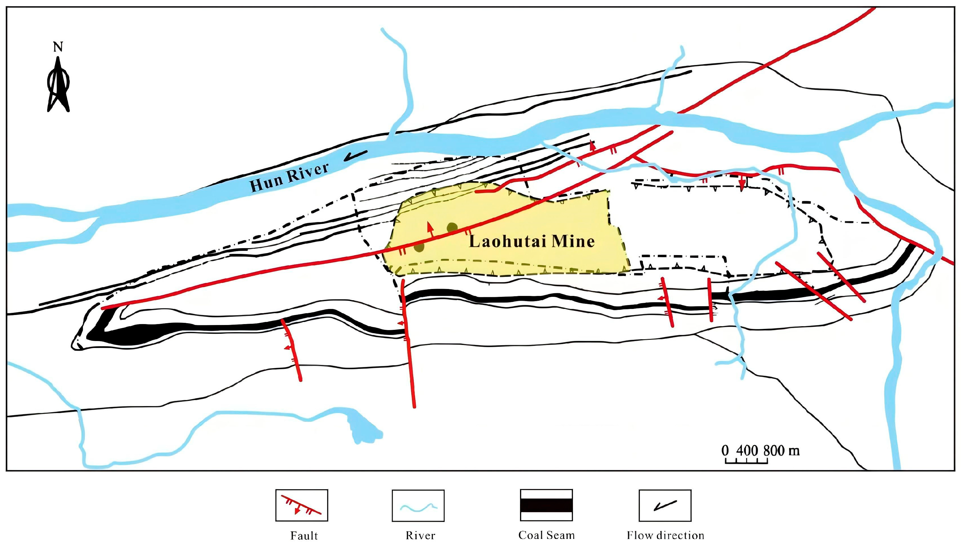
Figure 1. Regional location of the study area.
Water 16 02749 g001
Figure 2. Grid search-SARIMA–LSTM model flow chart.
Water 16 02749 g002
Figure 3. Hydrogeological generalization map.
Water 16 02749 g003
Figure 4. Partitioning of the numerical simulation study area.
Water 16 02749 g004
Figure 5. Fitted water level data for observation wells: (a) Well No. 2, (b) Well No. 4.
Water 16 02749 g005aWater 16 02749 g005b
Figure 6. Regionalization of permeability coefficients for (a) alluvial sand and gravel aquifer, (b) marl aquifer, and (c) tuff basalt aquifer.
Water 16 02749 g006
Figure 7. Changes in water head distributions of the alluvial sand and gravel aquifer.
Water 16 02749 g007
Figure 8. Numerical simulation water balance prediction result: (a) K Decrease, (b) K March, and (c) K Increase.
Water 16 02749 g008
Figure 9. Raw water inflow values.
Water 16 02749 g009
Figure 10. ACF and PACF diagrams.
Water 16 02749 g010
Figure 11. Grid search optimization of SARIMA before and after comparison diagram.
Water 16 02749 g011
Figure 12. Training SARIMA algorithm at various times.
Water 16 02749 g012
Figure 13. SARIMA predictive effectiveness.
Water 16 02749 g013
Figure 14. Predictions date of water inflow value prediction based on grid search-SARIMA-LSTM optimization model.
Water 16 02749 g014
Figure 15. Comparison of (a) Original Data and Predicted Values, and (b) Residual Distribution for VM and G-S-L Models.
Water 16 02749 g015aWater 16 02749 g015b
Table 1. Permeability coefficient.
Generalized StrataPermeability
Heterogeneity
Permeability Coefficient (m/d)Stratum Property
Alluvial Sand and Gravel Aquifer110.2Submerged Aquifer
211.6
312.4
419
Marl Aquifers50.0006Pressure Aquifer
60.001
Tuff Basalt Aquifers70.000028Pressure Aquifer
80.00005
Table 2. Root Mean Square Error (RMSE) of Training Data at Different Ratios.
DATARMSE
0.869.18227829955616
0.8582.79368072474763
0.985.38385786475945
Table 3. Best results of predicted monthly water inflow using the different approaches.
DATARMSER2
VMG-S-LVMG-S-L
2023-016858.028342−0.529143−0.304688
2023-022813.0843580.7407340.925511
2023-033426.2203730.6177140.659466
2023-049262.046975−1.799019−0.423810
2023-058269.788770−1.223606−0.697176
2023-066833.570071−0.5291430.541864
Disclaimer/Publisher’s Note: The statements, opinions and data contained in all publications are solely those of the individual author(s) and contributor(s) and not of MDPI and/or the editor(s). MDPI and/or the editor(s) disclaim responsibility for any injury to people or property resulting from any ideas, methods, instructions or products referred to in the content.