Article

Enhancing Evapotranspiration Estimations through Multi-Source Product Fusion in the Yellow River Basin, China

by
Runke Wang
*,
Xiaoni You
,
Yaya Shi
and
Chengyong Wu
School of Resources and Environmental Engineering, Tianshui Normal University, Tianshui 741001, China
*
Author to whom correspondence should be addressed.
Water 2024, 16(18), 2603; https://doi.org/10.3390/w16182603
Submission received: 10 August 2024 / Revised: 9 September 2024 / Accepted: 10 September 2024 / Published: 14 September 2024

Abstract

:
An accurate estimation of evapotranspiration (ET) is critical to understanding the water cycle in watersheds and promoting the sustainable utilization of water resources. Although there are various ET products in the Yellow River Basin, various ET products have many uncertainties due to input data, parameterization schemes, and scale conversion, resulting in significant uncertainties in regional ET data products. To reduce the uncertainty of a single product and obtain more accurate ET data, more accurate ET data can be obtained by fusing different ET data. Addressing this challenge, by calculating the uncertainty of three ET data products, namely global land surface satellite (GLASS) ET, Penman–Monteith–Leuning (PML)-V2 ET, and reliability-affordable averaging (REA) ET, the weight of each product is obtained to drive the Bayesian three-cornered Hat (BTCH) algorithm to obtain higher quality fused ET data, which are then validated at the site and basin scales, and the accuracy has significantly improved compared to a single input product. On a daily scale, the fused data’s root mean square error (RMSE) is 0.78 mm/day and 1.14 mm/day. The mean absolute error (MAE) is 0.53 mm/day and 0.84 mm/day, respectively, which has a lower RMSE and MAE than the model input data; the correlation coefficients (R) are 0.9 and 0.83, respectively. At the basin scale, the RMSE and MAE of the annual average ET of the fused data are 11.77 mm/year and 14.95 mm/year, respectively, and the correlation coefficient is 0.84. The results show that the BTCH ET fusion data are better than single-input product data. An analysis of the fused ET data on a spatiotemporal scale shows that from 2001 to 2017, the ET increased in 85.64% of the area of the Yellow River Basin. Fluctuations in ET were greater in the middle reaches of the Yellow River than in the upstream and downstream regions. The BTCH algorithm has indispensable reference value for regional ET estimation research, and the ET data after BTCH algorithm fusion have higher data quality than the original input data. The fused ET data can inform the development of management strategies for water resources in the YRB and provide a deeper understanding of the regional water supply and demand balance mechanism.

1. Introduction

Evapotranspiration (ET) is the process through which water vapor is released to the atmosphere from the earth’s surface and via plant transpiration. Following precipitation, ET is the second most significant component in the earth’s land-based water cycle [1,2]. Under the influence of global warming, the water cycle is predicted to intensify, increasing the global terrestrial ET [3]. As an important link in surface hydrothermal processes, the accurate estimation of ET is crucial for clarifying regional hydrological cycles [4], water resource management, irrigation planning [5], ecological environment changes [6], and socio-economic development research. Therefore, the accurate estimation of ET is of great theoretical significance for understanding and managing water resources and has practical significance in improving agricultural productivity, maintaining the ecosystem balance, and promoting regional socio-economic development. Through ET estimations, irrigation strategies can be optimized, drought and flood disasters can be predicted, and the impact of climate change on ecosystems can be assessed, thus providing key data support for sustainable development.
Due to challenges associated with observations and measurements, ET at the regional and global scales is typically obtained through model simulations [7,8], site observation data scaling [9,10], an empirical model [11,12], satellite remote sensing data inversion [13,14,15], data assimilation [16,17], machine learning [5,18], and deep learning [19]. Model simulation methods use physical and statistical models to estimate ET through calculations of surface and meteorological parameters. However, model simulations may amplify the ET estimation uncertainty due to the difficulty in obtaining the individual input parameters of the model and the algorithm or model sensitivity applied for indirect ET estimations. The station interpolation method for performing consistent ET spatiotemporal analysis using ground observation data is impeded by the uneven distribution of stations and inconsistent observation data spanning time. The empirical model establishes the relationship between ET and the main parameters related to ET estimations. Empirical methods are more accurate than complex models but typically require local calibration. Satellite remote sensing inversion technology offers an effective approach for estimating ET. Most relevant algorithms associate land surface variables obtained from satellite inversion with ET and ultimately obtain ET values via the estimation model. This method has the advantages of wide coverage and high temporal and spatial resolution, but its accuracy under complex surface conditions still needs to be further improved. The land surface energy balance model is a typical representative model that applies remote sensing data to ET estimations [20]. From the energy balance perspective, the one-source model (OSM) [21,22] and two-source energy balance (TSEB) model [13,23,24] represent and estimate ET as the residual term of the surface energy balance. When using OSM and TSEB models to estimate ET, the sensitivity to land surface temperature (LST) and air temperature depends on the land surface cover type, which may cause deviations in estimates. Notably, compared with the OSM model, the TSEB model exhibits better estimation accuracy [25]. Data-assimilation methods can improve the accuracy and consistency of ET estimates by fusing observational data and model simulation results. Still, its application is limited by the quality of data sources and the complexity of assimilation algorithms. In recent years, machine learning and deep learning technologies have been widely used in ET estimation due to their powerful data-processing and pattern-recognition capabilities. These methods can automatically learn complex nonlinear relationships between ET and related variables through large amounts of training data, significantly improving the estimation accuracy. However, different algorithms are highly dependent on the number of samples and data quality, and the generalization ability and representativeness of the model are still important challenges in research. Hence, using different methods to estimate the performance of ET remains a hot research topic [26].
While ET data can be obtained using different models and methods, many uncertainties exist in the model mechanism, input data, parameterization scheme, scale conversion, and other aspects, resulting in significant uncertainty in the regional ET data product output. The relative performances of different models on different underlying surfaces are inconsistent; accordingly, no globally optimal regional ET product is available. More accurate ET data can be obtained by fusing different ET data rather than using single-input data to reduce the uncertainty in a single product and obtain ET products with higher accuracy [27,28]. Data fusion is conducting a comprehensive analysis of data from various sources and extracting data with higher reliability than single data. The main methods of ET data fusion include the extended triple colonization (TC) fusion method [29], spatiotemporal adaptive method (STARFM) [30,31], and enhanced spatiotemporal adaptive fusion method (ESTARFM) [32]. The extended TC method is applied to MOD16, GLEAM, and GLDAS actual evapotranspiration products to develop a merged near-real-time accurate actual evapotranspiration dataset by dealing with theoretical and systematic uncertainties in the three actual evapotranspiration products. The advantage of this method is that the weights are adjusted according to the error structure of each dataset, thereby generating a more accurate and reliable dataset. However, this method strictly assumes that the errors of the three datasets are uncorrelated, orthogonal, and independent and are sensitive to the noise of the input data. The STARFM method integrates MODIS and Landsat data to estimate ET [33] or uses MODIS evapotranspiration products and ASTER satellite data to calculate the ET results [34]. While the STARFM method is suitable for homogeneous pixels with surface coverage, it has poor prediction performance for complex and heterogeneous underlying surfaces. The ESTARFM method achieves data fusion by improving the selection of similar pixels and weight calculations, which is suitable for data prediction in complex surface areas with high fusion accuracy. However, its computational complexity is relatively high, and computational resources and time costs must be considered. Previous studies have shown that for the spatiotemporal fusion of Sentinel-2 and MODIS data in typical areas of the Three-River Source, ESTARFM performed worse than STARFM under conditions where regional landscape heterogeneity did not change much [35].
Although the ET, as mentioned above, fusion models have made progress in estimating ET, previous studies have failed to consider the uncertainty of the input products. In the fusion process, only by considering the uncertainty of fusion between different products can the shortcomings of each product be avoided, and the global optimal ET dataset can be obtained after fusion. The Bayesian three-cornered hat (BTCH) algorithm [36] considers the uncertainty of different input ET datasets. Therefore, an exhaustive analysis and evaluation of the uncertainty of each input product is required before implementing fusion. The uncertainty is evaluated using error variance analysis, and the error variance is implemented using the three-connected hat (TCH) algorithm. The results show that mean ET data had significantly reduced errors than the parent products [37]. The advantage of the BTCH method is that it requires no prior knowledge. Data weights can be automatically assigned based on an uncertainty assessment, thus effectively reducing the uncertainty caused by a single data source. The results of the BTCH method in fusing different ET product data in the United States show that BTCH can capture the seasonal changes in ET estimates more accurately, and the long-term total water storage anomaly (TWSA) of the Mississippi River Basin (MRB) is calculated using BTCH-fused ET data. The results are consistent with the GRACE retrieval results [36]. This indicates that the BTCH method can provide more accurate ET data, making significant improvements to traditional fusion methods and overcoming the challenges of uncertainty and data quality. Fusion data can be used for regional water resource management and ecological protection.
The fusion of ET data in the study of the Yellow River Basin (YRB) can improve the accuracy and stability of ET estimations and provide key scientific support for regional water resource management in the basin. This has important scientific significance for supporting the implementation of ecological protection and high-quality development strategies in the YRB and ensuring water and ecological security in the YRB. Therefore, this study first evaluates the performance of different ET data products by calculating the uncertainty of different ET data products in China’s Yellow River Basin (YRB). Second, each product’s weight is obtained using the uncertainty calculation result, which drives the BTCH fusion algorithm and obtains the fusion ET data for the YRB, China. Finally, to validate the reliability of the ET fusion results, the validation was carried out based on the site location and the basin scale. The fusion results were validated during site validation using flux tower observation data. On the basin scale, the ET value obtained using the water balance method was used as the basin ET validation data [38]. The fused ET data were further analyzed to explore ET’s temporal and spatial variation trend.

2. Materials and Methods

2.1. Study Area

The Yellow River originates from the BaYan KaLa Mountains and flows into the Bohai Sea, with a total length of ~5464 km. The geographic range is 95.75° E–119.25° E and 32° N–42° N (Figure 1). According to the geographical location, the Yellow River is divided into the upper, middle, and lower reaches. The upstream portion extends from the river source to Toudaoguai, the midstream portion from Toudaoguai to Huayuankou, and the downstream portion from Huayuankou to the estuary. The upper region has a diverse geographical environment, including plateaus, mountains, and canyons, with a maximum height of 6119 m in the Digital Elevation Model (DEM). The middle reaches comprise the Loess Plateau, while the lower reaches largely contain the Yellow River alluvial plain. The YRB lies in a transitional zone between semi-arid and semi-humid climates, differing significantly from other watersheds in China [39]. The precipitation distribution in the YRB is heterogeneous, gradually decreasing from southeast to northwest. In terms of quantity, the precipitation in the basin’s upper, middle, and lower reaches is 368 mm, 562 mm, and 648 mm/year, respectively [40]. After China implemented high-quality development policies in the YRB, significant progress was made in this region’s ecological and environmental protection. Due to the government’s continued investment and innovative measures in watershed management and protection, the ecological security index of the YRB has gradually and steadily increased [41]. The land cover types in the study area are mainly grassland, cropland, forest, urban, and construction land, etc.
The study area included the capital cities of six provinces through which the Yellow River flows: Xining, Lanzhou, Yinchuan, Hohhot, Taiyuan, and Zhengzhou. The main hydrological monitoring stations include Tangnaihai, Lanzhou, and Toudaoguai [42] (Figure 1). The data that these hydrological stations provide is vital to monitoring water volume changes and analyzing water resource conditions in the YRB. The study area also included the Haibei shrub station and Haibei wetland station, part of the Chinese terrestrial ecosystem flux observation and research network (ChinaFLUX) (Figure 1).

2.2. Data and Processing

2.2.1. Remote Sensing Data and Preprocessing

Evapotranspiration Data Products

Three long-term series of ET data products, namely, global land surface satellite (GLASS) ET, Penman–Monteith–Leuning (PML)-V2 ET, and reliability-affordable averaging (REA) ET, served as the input data for the ET fusion algorithm. The GLASS ET had a spatial resolution of 1000 m (approximately 0.0083333°) and temporal resolution of 8 d, and the data are extended to the daily scale through interpolation. The validation results showed that the root mean square error (RMSE) of the GLASS ET products was <35.3 W/m2, better than that of MODIS ET [43]. For the China region, the PML-V2 dataset provided daily ET data with a spatial resolution of 500 m from 26 February 2000 to 31 December 2020 [44]. The REA ET used the reliability ensemble averaging method to obtain global daily ET data with a spatial resolution of 0.25° [45]. The PML-V2 ET and REA ET data were resampled to 0.0083333°, with the same spatial resolution as GLASS ET data. The daily ET values are accumulated to obtain monthly and annual ET values.

GRACE Data

The gravity recovery and climate experiment (GRACE) data were primarily reported by three research institutions: the University of Texas at the Austin Center for Space Research (CSR) in the United States, the Jet Propulsion Laboratory (JPL) of NASA, and the German Research Centre for Geosciences, Potsdam (GFZ). GRACE data are highly accurate, consistent with 2 cm between land and ocean, and have been used to evaluate regional and global trends in water storage changes [46,47]. This study selected the GRACE/GRACE-FO CSRRL06 Mascon V2 product terrestrial water storage anomaly (TWSA) from April 2002 to July 2017 with a monthly temporal resolution and 0.25° spatial resolution. To ensure the consistency of the data calculation, the bilinear interpolation method is used to resample the GRACE data to a spatial resolution of 0.0083333°.

2.2.2. Observed Data

The ET data observed at the site were sourced from the China National Ecological Science Data Service Center Resource Sharing Service Platform, which integrates long-term observation data from the China FLUX site from 2000 to 2010 with data from other observation sites in China [48]. The validation data are the observation data of the Haibei shrub station and Haibei wetland station. In this study, the observed daily latent heat flux data were converted into ET data based on the latent heat of evaporation parameters for the subsequent analysis. Based on each site’s geographic location information (latitude and longitude), extract the ET value of the pixel closest to the observation site, and then, compare the pixel value with the ET value observed at the site. The data used in the water balance method included average annual precipitation, measured runoff, and water inflow into the sea in the basin. Data were obtained from the Yellow River Water Resources Bulletin. In the basin-scale analysis, the ET data for the YRB were calculated based on the average precipitation and annual inflow into the sea.

2.3. Methods

In this paper, GLASS ET, PML-V2 ET, and REA ET data are used. Firstly, the uncertainty of each data product is calculated to determine the weight of each product. Then, the three input ET data were fused using the BTCH method, and the fusion results were validated. Finally, based on the fusion data, the temporal and spatial characteristics of ET in the study area are analyzed. The whole research process is divided into four steps: data preprocessing, weight calculation, ET data fusion and verification, and ET spatial and temporal change analysis (Figure 2).

2.3.1. Bayesian-Based Three-Cornered Hat Method

This study used the Bayesian three-cornered hat (BTCH) algorithm to fuse ET products [38]. The core assumption of the BTCH algorithm is that if the true value Xt of ET and the error standard of a certain ET product Xi are known, then the probability density function of the i th ET product E T i is
p ( E T i | E T t ) = 1 σ i 2 π exp [ ε i 2 2 σ i 2 ] = L ( E T t | E T i ) ( ε i = E T i E T t )
E T t denotes the true value of ET (actually, E T t is not available, and ETt is the hypothetical true value), L is a likelihood function, and ε i , and σ i are the zero-mean white noise and error variance of the i th ET product, respectively. The error variance σ i was solved using the three-connected hat (TCH) algorithm [37].
Similarly, if the true value of the X t of ET and the standard deviation of its error for a certain ET product X j can be determined by Equation (2)
p ( E T j | E T t ) = 1 σ j 2 π exp [ ε j 2 2 σ j 2 ] = L ( E T t | E T j ) ( ε j = E T j E T t )
where E T t denotes the true value of ET, L is a likelihood function, and ε j and σ j are the zero-mean white noise and error variance of the j th ET product, respectively, then the maximum likelihood of the true ET ( E T t ) is the maximum value of its joint probability distribution, as represented by Equation (3):
max L ( E T t | E T i , E T j ) = p ( E T i | E T t ) ( E T j | E T ) = 1 2 π σ i σ j exp [ ε i 2 2 σ i 2 ε j 2 2 σ j 2 ]
To obtain the maximum likelihood value of E T t the cost function J is defined by Equation (4):
J ( E T t ) = ε i 2 2 σ i 2 + ε j 2 2 σ j 2 = 1 2 [ [ E T i E T t ] 2 σ i 2 + [ E T j E T t ] 2 σ j 2 ]
Solving for the minimum value of Equation (4), that is, set the value of J ( E T t ) to zero, E T t can be expressed by Equation (5):
E T t = σ i 2 σ i 2 + σ j 2 E T i + σ j 2 σ i 2 + σ j 2 E T j
Define E T t = w i E T i + w j E T j , then
w i = σ i 2 σ i 2 + σ j 2 ,                   w j = σ j 2 σ i 2 + σ j 2
Similarly, E T t can be obtained using E T t = w 1 E T 1 + + w N E T N when N sets of ET products exist. The weight of each ET product can be obtained by minimizing a similar cost function (Equation (4)) and setting the weight w k according to Equation (7):
w k = i = 1 , i k N σ i 2 k = 1 N ( i = 1 , i k N σ i 2 )
The true value E T t can be solved using Equation (8):
X t = w 0 X 0 + w 1 X 1 + + w N X N
X t represents the ET value after fusion ( E T t ), X N the value of the Nth ET product, and w N the weight of the Nth product.

2.3.2. Water Balance Method

In a closed watershed, the water balance equation is the most effective for calculating the actual ET at the watershed scale [38]; the formula is represented by Equation (9):
E T w = P R Δ S
where ETw is the annual average ET of the watershed (mm/year), P is the average precipitation of the watershed (mm/year), and R is the runoff depth of the watershed (mm/year). ΔS is the annual change in watershed water reserves (mm/year), including surface and groundwater reserves, calculated using the GRACE satellite water reserve data [49]. However, on a multi-year scale (>10 years), changes in land water reserves can be ignored. Therefore, the calculation results of E T w can be used as reference data to validate the accuracy of ET estimations in the watershed [50].

2.3.3. Surface Energy Balance Closure

When studying the energy balance in the soil–vegetation–atmosphere system, ET is a key process involving water exchange and energy absorption. ET is typically expressed as LE in this system, with L representing the latent heat of vaporization. In the soil vegetation atmosphere energy balance system, the difference between the land surface net radiation (Rn) and soil heat flux (G) (available energy: RnG) is approximately equal to the sum of the sensible heat flux (H) and LE (turbulent flux: LE + H) [51]. Hence, the energy balance ratio (EBR, EBR = (LE + H)/(RnG)) for the turbulent energy flux to available energy is ~1.0.

2.3.4. Result Evaluation Method

Spatio-Temporal Scale Analysis Method

To quantify the changes in LST and air temperature in time and space, the least square linear regression method was used to calculate the slope of the unary linear equation of LST and air temperature from 2001 to 2020. The slope was the interannual change rate k; a k > 0 represents an upward trend; a k < 0 represents a downward trend. The calculation formula is presented in Equation (10) [52,53]:
k = u = 1 m ( u T u ) u = 1 m u u = 1 m T u / m u = 1 m u 2 ( u = 1 m u ) 2 / m
where u is the year serial number, Tu is the value of LST or air temperature corresponding to the year u, m is the research period, and m = 20.

Mann–Kendall Test

The Mann–Kendall test (M–K test) statistic S is represented by Equation (11) [54,55]:
S = i = 1 n 1 j = i + 1 n s i g n ( x j x i )
where n is the length of the dataset. xj and xj are the data values in the time series i and j (j > i), respectively; sign is the sign function.

Accuracy Evaluation Index

The RMSE, mean absolute error (MAE), mean absolute percentage error (MAPE), and correlation coefficient (R) provide different perspectives to evaluate the difference between calculated and observed values [56]. The smaller the MAPE, the closer the calculated value is to the observed value, whereas the opposite indicates lower accuracy for the calculated value. This study analyzed the correlations between ET data and the NDVI, temperature, and precipitation data using R, where a correlation coefficient (R) > 0 indicated a positive correlation between variables; otherwise, a negative correlation was identified.

3. Results

3.1. Uncertainty Analysis of Input Products

In the process of data fusion, ET products have potential uncertainties. Figure 3 shows the spatial distribution and uncertainty statistics of the average uncertainty of different ET products from 2001 to 2017. As can be seen from the figure, the product with the largest uncertainty is GLASS ET data (Figure 3a), followed by PML-V2 ET products (Figure 3b), while the uncertainty of REA ET products is smaller (Figure 3c). The uncertainty analysis of GLASS ET is relatively small in Lanzhou–Yinchuan–Hohhot. In the source area of the upper reaches of the Yellow River, the uncertainty of ET is greater than 1.1 mm/day. The uncertainty is highest in Lanzhou–Xi’an–Zhengzhou, greater than 1.2 mm/day. The uncertainty of PML-V2 ET data is the largest in Yinchuan in the upper reaches of the Yellow River, the uncertainty is smaller in Xining–Lanzhou in the upper reaches of the Yellow River, and the uncertainty is smaller in Xi’an–Taiyuan in the middle reaches of the Yellow River. The uncertainty of ET data in the lower reaches of the Yellow River is between 1.1 and 1.2 mm/day, and the uncertainty is relatively large. Between 2001 and 2017, the uncertainty of REA ET was relatively small, so in the fusion process, REA ET data had the largest weight. Figure 3d shows the statistical results of the uncertainty analysis of the three products. It can be seen from the figure that the uncertainties of GLASS and PML-V2 ET are relatively close under different underlying surfaces, which indicates that the methods and data sources used by these two products in calculating ET values may have similarities, and, therefore, show similar uncertainty levels under different environmental conditions. In contrast, the uncertainty of the REA ET product is the smallest, which means that the product has higher stability and reliability under various underlying surface conditions.
From the spatial distribution of each ET product, the uncertainty in Xi’an in the middle reaches of the Yellow River is relatively large, and the high uncertainty in Xi’an is mainly attributed to the development of urbanization. With the advancement of urbanization, the land use type in Xi’an has changed significantly, and the hydrological cycle system has also been significantly affected. Urbanization not only changes the surface vegetation cover and soil structure but also increases the use and impact of human activities on water resources. For example, the increase in urban buildings and infrastructure may change the precipitation flow path and soil moisture content, affecting evapotranspiration. In addition, the urban heat island effect may change local climate conditions, further increasing the uncertainty of evapotranspiration estimates.

3.2. Accuracy Validation

3.2.1. Validation of Site-Measured Data

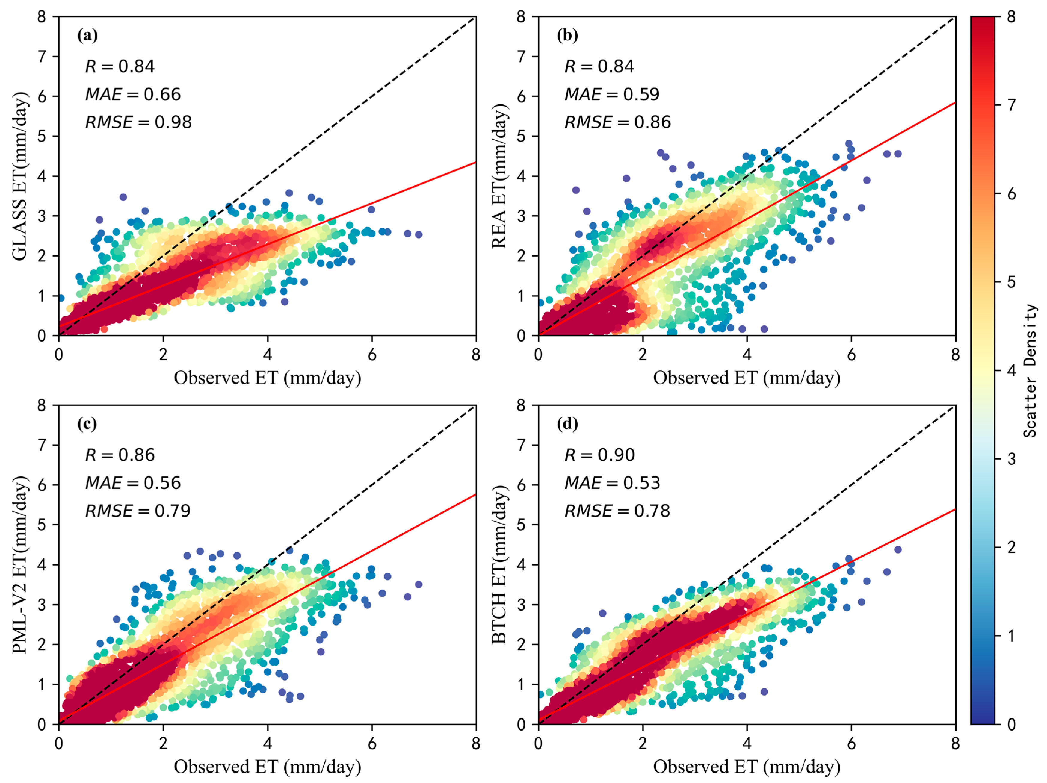
The accuracy validation results for the GLASS, REA, PML-V2 ET, and BTCH ET fusion datasets corresponding to the observation data from the Haibei shrub station from 2003 to 2010 are shown in a scatter density plot (Figure 4). As can be seen from Figure 4a–d, most of the data were concentrated between 0 and 2 mm/day. The RMSEs for the GLASS, REA, PML-V2, and BTCH ET datasets were 0.98, 0.86, 0.79, and 0.78 mm/day, respectively. The RMSE for the BTCH-fused ET is smaller than those for the GLASS, REA and PML-V2 data. Compared with the GLASS, REA, and PML-V2 ET RMSE, the BTCH ET RMSE decreased by 20.41%, 9.3%, and 1.27%. The MAEs for the GLASS, REA, PML-V2, and BTCH ET datasets were 0.66, 0.59, 0.56, and 0.53 mm/day, respectively. In comparison, the MAE of the BTCH ET data decreased by 19.7%, 10.17%, and 5.36%, respectively. The correlation coefficient R for the BTCH ET fusion dataset was 0.90, slightly higher than that of PML-V2, GLASS, and REA. Although the scatter plot in Figure 4 indicates that both PML-V2 ET and BTCH ET perform well, detailed data provided in the text reveal that BTCH ET demonstrates superior performance across various metrics. BTCH ET exhibits lower RMSE and MAE values and a higher correlation coefficient R, indicating that BTCH has the best accuracy on a daily scale when the land cover type is shrubs.
Figure 5 shows the analysis results of different ET data values compared to observed values at the Haibei wetland station in 2005. Figure 5a shows the relationship between daily ET observations and GLASS data, with RMSE, MAE, and R values of 0.94 mm/day, 1.27 mm/day, and 0.78, respectively. GLASS data tend to underestimate ET values greater than 4 mm/day. Figure 5b shows the relationship between daily ET observations and REA ET data, with RMSE, MAE, and R values of 0.89 mm/day, 1.22 mm/day, and 0.79, respectively. Higher ET measurements correspond to lower REA data values, but the overall error is slightly smaller than the GLASS ET data. Figure 5c shows the relationship between PML-V2 ET data and daily ET observations. The RMSE is 1.1 mm/day, MAE is 0.82 mm/day, and R is 0.8. The accuracy of PML-V2 data is higher than that of GLASS and REA ET data, and the error is smaller. Figure 5d depicts the relationship between daily ET values calculated using the BTCH model and observed values. The correlation coefficient R of the BTCH fused data is 0.83, higher than the data input based on the BTCH model, showing a strong positive correlation. The trend line is closer to the 1:1 line, but there is still deviation in areas with high ET values. BTCH ET data have an RMSE of 1.14 mm/day and MAE of 0.84 mm/day, slightly higher than PML-V2 ET data, but the difference is minor, showing good estimation accuracy. The validation results of the Haibei shrub and wetland station indicate that the BTCH fused data may vary across different land cover types. Nonetheless, the BTCH data fusion method is feasible.

3.2.2. Validation of Surface Energy Balance

A comparison of the calculated turbulence energy and available energy from the measured data at the Haibei shrub station is shown in Figure 6a. The coefficient R2 for the regression equation between the turbulent energy and available energy was 0.89. After removing data with an EBR > 1, the average ERB value was 0.88. Indeed, the ratio of turbulent flux to available energy observed at stations may not = 1.0 [57], and the turbulent flux is often smaller than the available energy [58].
A comparison between the turbulence energy calculated using the fused ET data and the available energy, with a determination coefficient R2 of 0.68, is shown in Figure 6b. When the available energy was <70 W/m2, the turbulent energy exceeded the available energy, whereas when the available energy was >70 W/m2, the available energy exceeded the turbulent energy, and the point was located below the 1:1 line. After removing the data with an EBR > 1.0, the average was 0.74, smaller than the EBR value calculated from the site observation data. Hence, the cause of energy non-closure warrants further investigation. This could be attributed to several reasons: (1) the spatial resolution of the ET products is 1 km, and validation using geographical coordinates and pixel scale effects should be fully considered; (2) the heat storage of the vegetation canopy in the research area cannot be ignored; (3) the lack of input parameters for calculating soil heat flux, meaning that only the influence of air temperature was considered when using the empirical formula recommended by the FAO to calculate soil heat flux [59], and the universality of the formula should be taken into account under different underlying surface conditions of the YRB.

3.2.3. Validation of the Water Balance Method

The annual average ET values for GLASS, REA, GLDAS, PML-V2, and BTCH products and the water balance ET value in the YRB from 2001 to 2017 were compared (Figure 7). The ET values for the GLASS products were lower than the observed values below the 1:1 line; the RMSE, MAE, and MAPE were 26.96 mm/year, 23.72 mm/year, and 5.34%, respectively (Figure 7a). The ET values for the REA products were significantly higher than the observed values, located far from the 1:1 line; the RMSE, MAE, and MAPE were 78.34 mm/year, 76.85 mm/year, and 17.6%, respectively. Hence, the REA ET overestimated the ET value of the watershed, as evidenced by the significant differences between results (Figure 7b). The ET values of the PML-V2 products were smaller than the observed values, with most points below the 1:1 line; the RMSE, MAE, and MAPE were 26.26 mm/year, 22.08 mm/year, and 4.95%, respectively (Figure 7c). Figure 5d shows that compared with GALSS, PML-V2, and REA ET data, the accuracy of BTCH ET fusion data has been improved, and the consistency is better, with RMSE, MAE, and MAPE of 14.95 mm/year, 11.77 mm/year, and 2.74%, respectively. The three products’ correlation coefficients (R) were 0.84, 0.76, and 0.66, respectively, and 0.84 for the BTCH ET fusion dataset. More points were distributed above the 1:1 line than below; however, the points were closer to the 1:1 line, and the observed and fused values were relatively close (Figure 7d). Overall, the ET data fused using the BTCH method in the YRB performed better than GLASS, REA, GLDAS, and PML-V2 ET products.

3.3. Spatiotemporal Variation Trends for Evapotranspiration

3.3.1. Characteristics of Evapotranspiration Time Variations

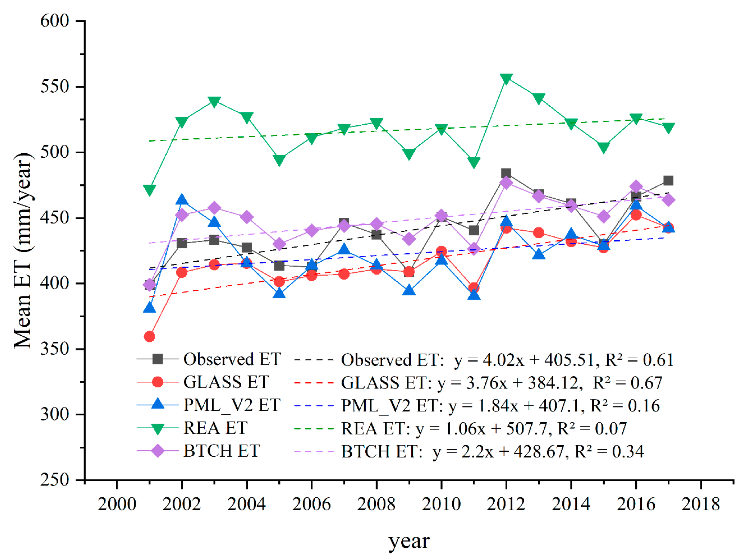
We used observational data from hydrological stations to drive the water balance method to calculate ET values at the basin scale as observed values. The average ET value in the YRB fluctuated between 350 and 550 mm from 2001 to 2017, with the average ET value in the REA products higher than that of the other ET products (Figure 8). The average ET values in the GLASS, PML-V2, and BTCH products were relatively close to those calculated from the observed values. The trends of observed values, GLASS, PML-V2, REA, and BTCH products were 4.02, 3.76, 1.84, 1.06, and 2.2 mm/year, respectively. The coefficients of determination R2 were 0.61, 0.67, 0.16, 0.07, and 0.34, respectively. The inter-annual changes among different ET products maintained consistency with an increasing trend. However, although PML-V2 and REA products also reflected interannual changes in ET, their performance was worse than that of the GLASS products and the fusion results of the BTCH method. Before 2007, the ET trend calculated from the observations was consistent with that of GLASS ET. After 2007, the ET trend calculated from the observations was consistent with that of the BTCH ET fusion dataset. The annual growth rate of integrated ET products was 2.2 mm/year. Before 2010, the BTCH ET value exceeded the observed value; after 2010, the BTCH ET value was lower than the observed value. The GLASS ET growth rate calculated from the watershed observations was the most rapid (growth rate: 3.76 mm/year); the REA ET product was the slowest (growth rate: 1.06 mm/year).

3.3.2. Spatial Variation Characteristics of Evapotranspiration

The annual average rate of change (k) for each pixel in the BTCH ET fusion dataset from 2003 to 2017 was calculated (Figure 9). From 2001 to 2017, the BTCH ET fusion data showed significant regional differences. The ET in most areas of the YRB exhibited increasing trends (k > 0), accounting for 85.64% of the basin area (Figure 9a). In the middle reaches of the Yellow River, the ET increased most rapidly between Toudaoguai and Longmen (annual growth rate: >5.0 mm/year), followed by the eastern area of Gansu Province, southern area of Ningxia Hui Autonomous Region, and northwestern area of Shaanxi Province (annual growth rate: >1.0 mm/year). The ET increased in some areas of the Qinghai and Sichuan Provinces, the source areas for the Yellow River; however, the growth rates in these areas were relatively low. The ET between Longmen and Huayuankou showed a decreasing trend, whereas that in the area from Huayuankou to the Yellow River estuary showed an increasing trend. Hence, spatial differences in ET are closely related to urban development [60], climate change, vegetation cover, and human activities [61].
The M-K method was used for significance testing to better understand the changes in BTCH ET from 2001 to 2017. The results showed that the regions connected by the Baiyin–Tianshui–Pingliang, Yulin–Yan’an and Linfen–Lvliang cities, with high interannual change rates, all passed the 95% significance test (Figure 9b), indicating an increasing trend in ET. In contrast, the Yellow River source area and most areas below Longmen did not pass the 95% significance test.

4. Discussion

By utilizing different models or algorithms, ET can be estimated. However, input parameters often constrain single-data products used in ET estimations. For instance, the TSEB model is particularly sensitive to surface and air temperature differences [13]. By analyzing the uncertainties of GLASS, PML-V2, and REA ET products, we found significant differences in the uncertainties of different ET products. This may be related to each product’s data source, algorithm, and sensitivity to land cover types. For example, GLASS and PML-V2 ET products have greater uncertainty in some urbanized development areas, which is related to the impact of urbanization on the surface vegetation cover and soil structure. In addition, the uncertainty of ET products is also affected by latitude [62], but in the Yellow River Basin, the impact of latitude is not obvious. Although combined with ground ET observation data, the weight of each ET product can be determined using statistical regression methods. The statistical regression method, however, assumes that the weight of the variables is based on empirical regression and that each input ET product is related to the result and does not consider the impact of each input ET product on the uncertainty of the fusion results. The BTCH method obtains an error covariance matrix for each ET product using the three-coordinate hat (TCH) method and then calculates the weights to obtain the fused ET data. The BTCH method considers the uncertainty of each product and assumes that the product with the least uncertainty contributes the most to the ET results. In this paper, the uncertainty of each ET product is not normalized, which avoids drastic fluctuations in ET fusion results caused by changes in uncertainty during data fusion.
A comparison of ET estimation methods, for instance, using machine learning techniques to improve land ET estimates in China from 2000 to 2018 demonstrated that machine learning can effectively enhance the ET estimation accuracy. However, the uneven distribution of ground observation stations may limit its applicability in barren areas [63]. In contrast, this study uses the BTCH fusion algorithm to calculate the uncertainty error of each input product, reflecting the level of understanding of unknown truth values. The results from the fusion process show that the accuracy for the BTCH ET products was improved, thus indicating that when comparing pixels at the same positions between different products, the fusion of ET data via the BTCH algorithm is more reliable when there is a small sample number. In the study of ET simulation optimization, previous researchers introduced data-driven models to improve the parameters in the physical process. They explored the optimization method of the ET zoning changes [64]. Their research emphasized the importance of a detailed evaluation of the uncertainty of ET data, which is consistent with the idea of this study. Both reduce the uncertainty of a single data source by integrating multiple data sources and improve the accuracy of the ET estimation. The difference is that the BTCH method is based on Bayesian analysis, in which different input ET products are regarded as random variables. The STARFM and ESTARFM methods have shown some application value in the ET estimation [30,32]. However, they exhibit limitations when dealing with complex and heterogeneous land cover. In contrast, the BTCH fusion algorithm, through the improved selection and weighting of similar pixels, is better suited for data prediction in complex surface areas, offering higher fusion accuracy.
Although the BTCH fusion algorithm performs well in improving the accuracy of the ET estimation, it still has some limitations. First, the BTCH method must be optimized for high computational complexity and resource consumption. Second, the fusion process is highly dependent on the quality of input data, and the reliability and consistency of the data source need to be ensured. In addition, for areas with strong surface heterogeneity, the accuracy of the fusion results still needs to be improved. Therefore, future research needs to further optimize the fusion algorithm, improve the computational efficiency, and expand the coverage of data sources to meet the challenges brought by more complex surface conditions and environmental changes.

5. Conclusions

The BTCH algorithm can be used to fuse multiple ET products; this study used it to merge the ET data for the YRB. The validation of the resulting site observation data showed that when compared with GLASS and REA ET data, the RMSE of the Haibei shrub station decreased by 20.41% and 9.3%, respectively, on a daily scale after fusion. Although PML-V2 ET and BTCH ET performed well in the scatter plot, BTCH ET showed superior performance in various indicators, including lower RMSE and MAE values and a higher correlation coefficient R, indicating its reliability and accuracy in ET estimations. The fusion method of the BTCH ET dataset demonstrates its applicability and feasibility under different land cover types, although the specific performance may vary depending on the land cover type. These results can be used to analyze the water reserves in the study area or as input data for other models.
The ET in 85.64% of the YRB showed an increasing trend from 2001 to 2017, but its distribution and growth rate in different regions showed significant differences. Specifically, the middle reaches of the Yellow River, from Toudaoguai to Longmen, exhibited the fastest increase in the ET rate, followed by the eastern area of the Gansu Province, the southern area of the Ningxia Hui Autonomous Region, and the northwestern area of the Shaanxi Province. The ET showed an increasing trend in some areas of Qinghai Province, the source area of the Yellow River, but the growth rate was relatively low. These results reveal the changing characteristics of ET in the YRB and provide key data to support and a scientific basis for analyzing the causes of changes in water resources in the YRB and the rational development and utilization of water resources in the basin.

Author Contributions

R.W.: conceptualization, methodology, writing of code, writing—original draft preparation. X.Y.: resources, experimental conception and design, writing—reviewing. Y.S.: data downloading and preprocessing. C.W.: investigation, validation. All authors have read and agreed to the published version of the manuscript.

Funding

This research was supported by the State Key Laboratory of Frozen Soil Engineering, Northwest Institute of Eco-Environment and Resources, Chinese Academy Sciences [grant number SKLFSE202014]; the Youth Science and Technology Fund of Gansu Provincial Science and Technology Department [grant number 23JRRE727]; the Science and Technology Program of Gansu Province [grant number 21JR1RE293, 22JR5R194]; and the Youth Doctoral Program in Higher Education Institutions of Gansu Province [grant number 2022QB-143].

Data Availability Statement

REA ET and PML-V2 ET data were obtained from the National Tibetan Plateau Data Center (https://data.tpdc.ac.cn/). The GLASS ET was derived from the GLASS products (http://www.glass.umd.edu/). Air temperature and precipitation data were obtained from the Science Data Bank (https://www.scidb.cn/en). GRACE data were obtained from the Jet Power Laboratory at JPL (search.earthdata.nasa.gov). The NDVI data were obtained from the Resource and Environment Science and Data Center (https://www.resdc.cn/). Site observational data were obtained from ChinaFLUX (http://www.chinaflux.org/).

Acknowledgments

We would like to acknowledge the China National Meteorological Service Center for supplying the meteorological data for this research.

Conflicts of Interest

The authors declare no conflicts of interest.

References

  1. Rodell, M.; Beaudoing, H.K.; L’ecuyer, T.S.; Olson, W.S.; Famiglietti, J.S.; Houser, P.R.; Adler, R.; Bosilovich, M.G.; Clayson, C.A.; Chambers, D.; et al. The observed state of the water cycle in the early twenty-first century. J. Clim. 2015, 28, 8289–8318. [Google Scholar] [CrossRef]
  2. Huang, Q.; Ma, N.; Wang, P. Faster increase in evapotranspiration in permafrost-dominated basins in the warming Pan-Arctic. J. Hydrol. 2022, 615, 128678. [Google Scholar] [CrossRef]
  3. Huntington, T.G. Evidence for intensification of the global water cycle: Review and synthesis. J. Hydrol. 2005, 319, 83–95. [Google Scholar] [CrossRef]
  4. Vergopolan, N.; Fisher, J.B. The impact of deforestation on the hydrological cycle in Amazonia as observed from remote sensing. Int. J. Remote Sens. 2016, 37, 5412–5430. [Google Scholar] [CrossRef]
  5. Granata, F. Evapotranspiration evaluation models based on machine learning algorithms—A comparative study. Agric. Water Manag. 2019, 217, 303–315. [Google Scholar] [CrossRef]
  6. Zhao, F.; Ma, S.; Wu, Y.; Qiu, L.; Wang, W.; Lian, Y.; Chen, J.; Sivakumar, B. The role of climate change and vegetation greening on evapotranspiration variation in the Yellow River Basin, China. Agric. For. Meteorol. 2022, 316, 108842. [Google Scholar] [CrossRef]
  7. Monin, A.S.; Obukhov, A.M. Basic laws of turbulent mixing in the surface layer of the atmosphere. Contrib. Geophys. Inst. Acad. Sci. USSR 1954, 24, 163–187. [Google Scholar]
  8. Penman, H.L. Natural evaporation from open water, bare soil and grass. Proc. R. Soc. Lond. Ser. A 1948, 193, 120–145. [Google Scholar] [CrossRef]
  9. Wilson, K.; Goldstein, A.; Falge, E.; Aubinet, M.; Baldocchi, D.; Berbigier, P.; Bernhofer, C.; Ceulemans, R.; Dolman, H.; Field, C.; et al. Energy balance closure at FLUXNET sites. Agric. For. Meteorol. 2002, 113, 223–243. [Google Scholar] [CrossRef]
  10. Baldocchi, D. ‘Breathing’ of the terrestrial biosphere: Lessons learned from a global network of carbon dioxide flux measurement systems. Aust. J. Bot. 2008, 56, 1–26. [Google Scholar] [CrossRef]
  11. Anderson, R.G.; Goulden, M.L. A mobile platform to constrain regional estimates of evapotranspiration. Agric. For. Meteorol. 2009, 149, 771–782. [Google Scholar] [CrossRef]
  12. Wang, K.; Liang, S. An improved method for estimating global evapotranspiration based on satellite determination of surface net radiation, vegetation index, temperature, and soil moisture. J. Hydrometeorol. 2008, 9, 712–727. [Google Scholar] [CrossRef]
  13. Norman, J.M.; Kustas, W.P.; Humes, K.S. Source approach for estimating soil and vegetation energy fluxes in observations of directional radiometric surface temperature. Agric. For. Meteorol. 1995, 77, 263–293. [Google Scholar] [CrossRef]
  14. Su, Z. The Surface Energy Balance System (SEBS) for estimation of turbulent heat fluxes. Hydrol. Earth Syst. Sci. 2002, 6, 85–99. [Google Scholar] [CrossRef]
  15. Jiang, L.; Islam, S. Estimation of surface evaporation map over southern Great Plains using remote sensing data. Water Resour. Res. 2001, 37, 329–340. [Google Scholar] [CrossRef]
  16. Caparrini, F.; Castelli, F.; Entekhabi, D. Estimation of surface turbulent fluxes through assimilation of radiometric surface temperature sequences. J. Hydrometeorol. 2004, 5, 145–159. [Google Scholar] [CrossRef]
  17. Deb, P.; Abbaszadeh, P.; Moradkhani, H. An ensemble data assimilation approach to improve farm-scale actual evapotranspiration estimation. Agric. For. Meteorol. 2022, 321, 108982. [Google Scholar] [CrossRef]
  18. Xu, T.; Guo, Z.; Liu, S.; He, X.; Meng, Y.; Xu, Z.; Xia, Y.; Xiao, J.; Zhang, Y.; Ma, Y.; et al. Evaluating different machine learning methods for upscaling evapotranspiration from flux towers to the regional scale. J. Geophys. Res. Atmos. 2018, 123, 8674–8690. [Google Scholar] [CrossRef]
  19. Chen, Z.; Zhu, Z.; Jiang, H.; Sun, S. Estimating daily reference evapotranspiration based on limited meteorological data using deep learning and classical machine learning methods. J. Hydrol. 2020, 591, 125286. [Google Scholar] [CrossRef]
  20. Morillas, L.; García, M.; Nieto, H.; Villagarcia, L.; Sandholt, I.; Gonzalez-Dugo, M.; Zarco-Tejada, P.; Domingo, F. Using radiometric surface temperature for surface energy flux estimation in Mediterranean drylands from a two-source perspective. Remote Sens. Environ. 2013, 136, 234–246. [Google Scholar] [CrossRef]
  21. Kustas, W.P.; Daughtry, C.S.; Van Oevelen, P.J. Analytical treatment of the relationships between soil heat flux/net radiation ratio and vegetation indices. Remote Sens. Environ. 1993, 46, 319–330. [Google Scholar] [CrossRef]
  22. Jacobsen, A.; Hansen, B.U. Estimation of the soil heat flux/net radiation ratio based on spectral vegetation indexes in high-latitude Arctic areas. Int. J. Remote Sens. 1999, 20, 445–461. [Google Scholar] [CrossRef]
  23. Dolman, A.J. A multiple-source land surface energy balance model for use in general circulation models. Agric. For. Meteorol. 1993, 65, 21–45. [Google Scholar] [CrossRef]
  24. Shuttleworth, W.J.; Wallace, J.S. Evaporation from sparse crops-an energy combination theory. Q. J. R. Meteorol. Soc. 1985, 111, 839–855. [Google Scholar] [CrossRef]
  25. Wang, R.; Wang, J.; Zhu, G.; Li, H.; Shao, D.; Hao, X. Estimation of surface latent heat fluxes in an oasis utilizing a two-source energy balance model based on land surface temperature decomposition. J. Appl. Remote Sens. 2019, 13, 034504. [Google Scholar] [CrossRef]
  26. Yaseen, Z.M.; Al-Juboori, A.M.; Beyaztas, U.; Al-Ansari, N.; Chau, K.-W.; Qi, C.; Ali, M.; Salih, S.Q.; Shahid, S. Prediction of evaporation in arid and semi-arid regions: A comparative study using different machine learning models. Eng. Appl. Comput. Fluid Mech. 2019, 14, 70–89. [Google Scholar] [CrossRef]
  27. Jiménez, C.; Martens, B.; Miralles, D.M.; Fisher, J.B.; Beck, H.E.; Fernández-Prieto, D. Exploring the merging of the global land evaporation WACMOS-ET products based on local tower measurements. Hydrol. Earth Syst. Sci. 2018, 22, 4513–4533. [Google Scholar] [CrossRef]
  28. Yao, Y.; Liang, S.; Li, X.; Hong, Y.; Fisher, J.B.; Zhang, N.; Chen, J.; Cheng, J.; Zhao, S.; Zhang, X.; et al. Bayesian multimodel estimation of global terrestrial latent heat flux from eddy covariance, meteorological, and satellite observations. J. Geophys. Res. Atmos. 2014, 119, 4521–4545. [Google Scholar] [CrossRef]
  29. Khan, M.S.; Liaqat, U.W.; Baik, J.; Choi, M. Stand-alone uncertainty characterization of GLEAM, GLDAS and MOD16 evapotranspiration products using an extended triple collocation approach. Agric. For. Meteorol. 2018, 252, 256–268. [Google Scholar] [CrossRef]
  30. Cammalleri, C.; Anderson, M.; Gao, F.; Hain, C.; Kustas, W. Mapping daily evapotranspiration at field scales over rainfed and irrigated agricultural areas using remote sensing data fusion. Agric. For. Meteorol. 2014, 186, 1–11. [Google Scholar] [CrossRef]
  31. Gao, F.; Masek, J.; Schwaller, M.; Hall, F. On the blending of the Landsat and MODIS surface reflectance: Predicting daily Landsat surface reflectance. IEEE Trans. Geosci. Remote 2006, 44, 2207–2218. [Google Scholar] [CrossRef]
  32. Zhu, X.; Chen, J.; Gao, F.; Chen, X.; Masek, J.G. An enhanced spatial and temporal adaptive reflectance fusion model for complex heterogeneous regions. Remote Sens. Environ. 2010, 114, 2610–2623. [Google Scholar] [CrossRef]
  33. Yang, Y.; Anderson, M.C.; Gao, F.; Hain, C.R.; Semmens, K.A.; Kustas, W.P.; Noormets, A.; Wynne, R.H.; Thomas, V.A.; Sun, G. Daily Landsat-scale evapotranspiration estimation over a forested landscape in North Carolina, USA, using multi-satellite data fusion. Hydrol. Earth Syst. Sci. 2017, 21, 1017–1037. [Google Scholar] [CrossRef]
  34. Yi, Z.; Zhao, H.; Jiang, Y. Continuous daily evapotranspiration estimation at the field-scale over heterogeneous agricultural areas by fusing ASTER and MODIS data. Remote Sens. 2018, 10, 1694. [Google Scholar] [CrossRef]
  35. Fan, M.; Ma, D.; Huang, X.; An, R. Adaptability Evaluation of the Spatiotemporal Fusion Model of Sentinel-2 and MODIS Data in a Typical Area of the Three-River Headwater Region. Sustainability 2023, 15, 8697. [Google Scholar] [CrossRef]
  36. He, X.; Xu, T.; Xia, Y.; Bateni, S.M.; Guo, Z.; Liu, S.; Mao, K.; Zhang, Y.; Feng, H.; Zhao, J. A Bayesian three-cornered hat (BTCH) method: Improving the terrestrial evapotranspiration estimation. Remote Sens. 2020, 12, 878. [Google Scholar] [CrossRef]
  37. Koot, L.; Viron, O.D.; Dehant, V. Atmospheric angular momentum time-series: Characterization of their internal noise and creation of a combined series. J. Geodesy 2006, 79, 663–674. [Google Scholar] [CrossRef]
  38. Long, D.; Longuevergne, L.; Scanlon, B.R. Uncertainty in evapotranspiration from land surface modeling, remote sensing, and GRACE satellites. Water Resour. Res. 2014, 50, 1131–1151. [Google Scholar] [CrossRef]
  39. Zhu, Y.; Chang, J.; Huang, S.; Huang, Q. Characteristics of integrated droughts based on a nonparametric standardized drought index in the Yellow River Basin, China. Hydrol. Res. 2015, 47, 454–467. [Google Scholar] [CrossRef]
  40. Chang, J.; Wei, J.; Wang, Y.; Yuan, M.; Guo, J. Precipitation and runoff variations in the Yellow River Basin of China. J. Hydroinform. 2016, 19, 138–155. [Google Scholar] [CrossRef]
  41. Qiu, M.; Zuo, Q.; Wu, Q.; Yang, Z.; Zhang, J. Water ecological security assessment and spatial autocorrelation analysis of prefectural regions involved in the Yellow River Basin. Sci. Rep. 2022, 12, 5105. [Google Scholar] [CrossRef]
  42. Wang, F.; Wang, Z.; Yang, H.; Di, D.; Zhao, Y.; Liang, Q.; Hussain, Z. Comprehensive evaluation of hydrological drought and its relationships with meteorological drought in the Yellow River basin, China. J. Hydrol. 2020, 584, 124751. [Google Scholar] [CrossRef]
  43. Liang, S.; Cheng, J.; Jia, K.; Jiang, B.; Liu, Q.; Xiao, Z.; Yao, Y.; Yuan, W.; Zhang, X.; Zhao, X.; et al. The Global land surface satellite (GLASS) product suite. Bull. Am. Meteorol. Soc. 2021, 102, E323–E337. [Google Scholar] [CrossRef]
  44. He, S.; Zhang, Y.; Ma, N.; Tian, J.; Kong, D.; Liu, C. A daily and 500 m coupled evapotranspiration and gross primary production product across China during 2000–2020. Earth Syst. Sci. Data 2022, 14, 5463–5488. [Google Scholar] [CrossRef]
  45. Lu, J.; Wang, G.; Chen, T.; Li, S.; Hagan, D.F.T.; Kattel, G.; Peng, J.; Jiang, T.; Su, B. A harmonized global land evaporation dataset from model-based products covering 1980–2017. Earth Syst. Sci. Data 2021, 13, 5879–5898. [Google Scholar] [CrossRef]
  46. Voss, K.A.; Famiglietti, J.S.; Lo, M.-H.; De Linage, C.; Rodell, M.; Swenson, S.C. Groundwater depletion in the Middle East from GRACE with implications for transboundary water management in the Tigris-Euphrates-Western Iran region. Water Resour. Res. 2013, 49, 904–914. [Google Scholar] [CrossRef]
  47. Xu, L.; Chen, N.; Zhang, X.; Chen, Z. Spatiotemporal changes in China’s terrestrial water storage from GRACE satellites and its possible drivers. J. Geophys. Res. Atmos. 2019, 124, 11976–11993. [Google Scholar] [CrossRef]
  48. Zheng, H.; Yu, G.; Zhu, X.; Wang, Q.; Zhang, L.; Chen, Z.; Sun, X.; He, H.; Su, W.; Wang, Y.; et al. A Dataset of Actual Evapotranspiration and Water Use Efficiency of Typical Terrestrial Ecosystems in China (2000–2010); China Scientific Data: Beijing, China, 2019. [Google Scholar] [CrossRef]
  49. Chen, H.; Zhang, W.; Nie, N.; Guo, Y. Long-term groundwater storage variations estimated in the Songhua River Basin by using GRACE products, land surface models, and in-situ observations. Sci. Total. Environ. 2018, 649, 372–387. [Google Scholar] [CrossRef]
  50. Velpuri, N.M.; Senay, G.B.; Singh, R.K.; Bohms, S.; Verdin, J.P. A comprehensive evaluation of two MODIS evapotranspiration products over the conterminous United States: Using point and gridded FLUXNET and water balance ET. Remote Sens. Environ. 2013, 139, 35–49. [Google Scholar] [CrossRef]
  51. Colaizzi, P.D.; Evett, S.R.; Howell, T.A.; Gowda, P.H.; Oâshaughnessy, S.A.; Tolk, J.A.; Kustas, W.P.; Anderson, M.C. Two-source energy balance model: Refinements and lysimeter tests in the southern high plains. Trans. ASABE 2012, 55, 551–562. [Google Scholar] [CrossRef]
  52. Song, Z.; Yang, H.; Huang, X.; Yu, W.; Huang, J.; Ma, M. The spatiotemporal pattern and influencing factors of land surface temperature change in China from 2003 to 2019. Int. J. Appl. Earth Obs. 2021, 104, 102537. [Google Scholar] [CrossRef]
  53. Wang, R.; You, X.; Shi, Y.; Wu, C.; Liu, B. Study on air temperature estimation and its influencing factors in a complex mountainous area. PLoS ONE 2022, 17, e0272946. [Google Scholar] [CrossRef]
  54. Sonali, P.; Kumar, D.N. Review of trend detection methods and their application to detect temperature changes in India. J. Hydrol. 2013, 476, 212–227. [Google Scholar] [CrossRef]
  55. Bari, S.H.; Rahman, M.T.U.; Hoque, M.A.; Hussain, M. Analysis of seasonal and annual rainfall trends in the northern region of Bangladesh. Atmospheric Res. 2016, 176–177, 148–158. [Google Scholar] [CrossRef]
  56. Willmott, C.J. Some comments on the evaluation of model performance. B. Am. Meteorol. Soc. 1982, 63, 1309–1313. [Google Scholar] [CrossRef]
  57. Liu, S.M.; Xu, Z.W.; Wang, W.Z.; Jia, Z.Z.; Zhu, M.J.; Bai, J.; Wang, J.M. A comparison of eddy-covariance and large aperture scintillometer measurements with respect to the energy balance closure problem. Hydrol. Earth Syst. Sci. 2011, 15, 1291–1306. [Google Scholar] [CrossRef]
  58. Barr, A.; Morgenstern, K.; Black, T.; McCaughey, J.; Nesic, Z. Surface energy balance closure by the eddy-covariance method above three boreal forest stands and implications for the measurement of the CO2 flux. Agric. For. Meteorol. 2006, 140, 322–337. [Google Scholar] [CrossRef]
  59. Allen, R.G.; Pereira, L.S.; Raes, D.; Smith, M. Crop Evapotranspiration-Guidelines for Computing Crop Water Requirements; FAO Irrigation and drainage paper 56; FAO: Rome, Italy, 1998; pp. 17–64. [Google Scholar]
  60. Hasan, A.; Mia, B.; Khan, M.R.; Alam, J.; Chowdury, T.; Amin, A.; Ahmed, K.M.U. Temporal changes in land cover, land surface temperature, soil moisture, and evapotranspiration using remote sensing techniques—A case study of Kutupalong rohingya refugee camp in Bangladesh. J. Geovisualization Spat. Anal. 2023, 7, 11. [Google Scholar] [CrossRef]
  61. Liu, Y.; Gui, D.; Yin, C.; Zhang, L.; Xue, D.; Liu, Y.; Ahmed, Z.; Zeng, F. Effects of Human Activities on Evapotranspiration and Its Components in Arid Areas. Int. J. Environ. Res. Public Health 2023, 20, 2795. [Google Scholar] [CrossRef]
  62. Cui, Z.; Zhang, Y.; Wang, A.; Wu, J.; Li, C. Uncertainty Analysis and Data Fusion of Multi-Source Land Evapotranspiration Products Based on the TCH Method. Remote Sens. 2023, 16, 28. [Google Scholar] [CrossRef]
  63. Yin, L.; Tao, F.; Chen, Y.; Liu, F.; Hu, J. Improving terrestrial evapotranspiration estimation across China during 2000–2018 with machine learning methods. J. Hydrol. 2021, 600, 126538. [Google Scholar] [CrossRef]
  64. Jiang, X.; Wang, Y.; Yinglan, A.; Wang, G.; Zhang, X.; Ma, G.; Duan, L.; Liu, K. Optimizing actual evapotranspiration simulation to identify evapotranspiration partitioning variations: A fusion of physical processes and machine learning techniques. Agric. Water Manag. 2024, 295, 108755. [Google Scholar] [CrossRef]
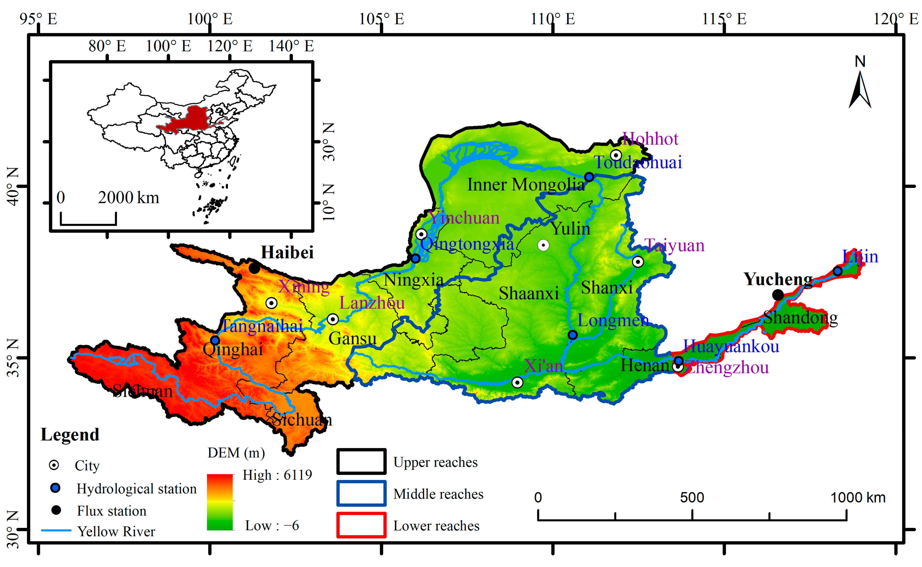
Figure 1. Location of the research area and distribution of major cities, hydrological stations, and flux observation stations.
Water 16 02603 g001
Figure 2. Technical flowchart.
Water 16 02603 g002
Figure 3. Uncertainty results of different evapotranspiration products, (a) GLASS ET, (b) PML-V2 ET, (c) REA ET, and (d) uncertainty statistics.
Water 16 02603 g003
Figure 4. Accuracy validation of ET products, fusion ET data, and flux tower data at Haibei shrub station from 2003 to 2010. (a) GLASS, (b) REA, (c) PML-V2, (d) BTCH (red: fitting line; dashed: best-fit line, a 1:1 line).
Water 16 02603 g004
Figure 5. Accuracy validation of ET products, fusion ET data, and flux tower data at Haibei wetland station in 2005. (a) GLASS, (b) REA, (c) PML-V2, (d) BTCH (red: fitting line; dashed: best-fit line, a 1:1 line).
Water 16 02603 g005
Figure 6. Energy balance ratio of observed data and fused ET data from the Haibei shrub station. (a) measured data, (b) fused ET data.
Water 16 02603 g006
Figure 7. Comparison of the average and observed values for ET from the different products in the YRB. (a) GLASS, (b) REA, (c) PML-V2, (d) BTCH.
Water 16 02603 g007
Figure 8. Variation characteristics for the average values of different ET products in the YRB.
Water 16 02603 g008
Figure 9. Interannual ET change rate (a) and M-K significance test (b) of BTCH fusion from 2001 to 2017.
Water 16 02603 g009
Disclaimer/Publisher’s Note: The statements, opinions and data contained in all publications are solely those of the individual author(s) and contributor(s) and not of MDPI and/or the editor(s). MDPI and/or the editor(s) disclaim responsibility for any injury to people or property resulting from any ideas, methods, instructions or products referred to in the content.