Article

Flood Susceptibility Assessment for Improving the Resilience Capacity of Railway Infrastructure Networks

1
Department of Engineering, Parthenope University, 80143 Naples, Italy
2
Research Centre, Ferrovie dello Stato Italiane S.p.A., 50123 Florence, Italy
3
Research Centre, Ferrovie dello Stato Italiane S.p.A., 00161 Rome, Italy
4
Technical Department, Rete Ferroviaria Italiana (RFI) S.p.A., 00161 Rome, Italy
5
School of Engineering, College of Arts, Technology and Environment, University of the West of England (UWE), Bristol BS16 1QY, UK
6
School of Architecture and Environment, College of Arts, Technology and Environment, University of the West of England (UWE), Bristol BS16 1QY, UK
7
College of Arts, Technology and Environment, University of the West of England (UWE), Bristol BS16 1QY, UK
*
Authors to whom correspondence should be addressed.
Water 2024, 16(18), 2592; https://doi.org/10.3390/w16182592
Submission received: 30 July 2024 / Revised: 1 September 2024 / Accepted: 10 September 2024 / Published: 12 September 2024

Abstract

:
Floods often cause significant damage to transportation infrastructure such as roads, railways, and bridges. This study identifies several topographic, environmental, and hydrological factors (slope, elevation, rainfall, land use and cover, distance from rivers, geology, topographic wetness index, and drainage density) influencing the safety of the railway infrastructure and uses multi-criteria analysis (MCA) alongside an analytical hierarchy process (AHP) to produce flood susceptibility maps within a geographic information system (GIS). The proposed methodology was applied to the catchment area of a railway track in southern Italy that was heavily affected by a destructive flood that occurred in the autumn of 2015. Two susceptibility maps were obtained, one based on static geophysical factors and another including triggering rainfall (dynamic). The results showed that large portions of the railway line are in a very highly susceptible zone. The flood susceptibility maps were found to be in good agreement with the post-disaster flood-induced infrastructural damage recorded along the railway, whilst the official inundation maps from competent authorities fail to supply information about flooding occurring along secondary tributaries and from direct rainfall. The reliable identification of sites susceptible to floods and damage may provide railway and environmental authorities with useful information for preparing disaster management action plans, risk analysis, and targeted infrastructure maintenance/monitoring programs, improving the resilience capacity of the railway network. The proposed approach may offer railway authorities a cost-effective strategy for rapidly screening flood susceptibility at regional/national levels and could also be applied to other types of linear transport infrastructures.

1. Introduction

Rail infrastructure networks are critical transport arteries that sustain mobility in contemporary society, underpinning economic and social well-being [1,2]. In recent years, climate change has led to an increased frequency and severity of extreme weather events [3], which have adversely affected railway infrastructure and its associated operations [4]. For example, intense precipitation has caused direct damage to the functioning of electrical systems, destabilized railway embankments, and triggered geohydrological hazards (i.e., landslides and floods) that have destroyed physical assets (i.e., tracks, tunnels, bridges) and, concomitantly, disrupted rail services and traffic flows [2,5,6,7].
Vulnerabilities to climate change increase the socio-economic costs and reduce the reliability of railway transportation [8,9]. Throughout Europe, and most notably across Italy, geohydrological hazards (i.e., landslides and floods) are widespread phenomena that constitute a detrimental influence on the built environment and transportation infrastructure [10,11,12,13,14]. Ref. [10] estimate that ~15% of the Italian railway network is exposed to landslides and ~24% to floods. Uncertainty in these estimates arises because of the extensive nature of the network and the cost of undertaking a comprehensive assessment. Past analysis has been mainly confined to major rivers and the most critical sections [10,15]. A cost-effective approach to screening hazards of this nature is therefore a critical need.
Flooding can derive from various sources including intense and/or persistent rainfall, high river flows, and coastal storms [16]. Fluvial (or riverine) flooding occurs when river water levels rise and overflow onto their adjacent floodplains [17]. Pluvial (or surface) flooding arises from rain-induced overland flow, resulting in local accumulations of water before the runoff enters any river or drainage facility or when it cannot enter these systems due to reduced capacity or blockage [18,19]. Flash floods combine both pluvial and fluvial elements, typically impact small steep watersheds, and are characterized by rapid flow velocities that may lead to debris flows, significant sediment transport, and erosion [19]. Railway–river intersections, or locations where culverts and ditches are obstructed by debris and sediment material, are therefore vulnerable points for railway network infrastructure. The inundation of railway tracks due to water flow can result in issues such as washing away of ballast, slope instability, and embankment breaches [7]. Water-induced damage on rail infrastructure can necessitate extensive and expensive repair work and involve temporary redirecting of trains in the case of link disruption, a scenario more pronounced in rail systems when compared to competing road networks due to their complex interconnected nature and poor flexibility [9,20].
Rail (and environmental) authorities require methodologies that enable rapid spatial assessment of the flood hazards that affect railway infrastructure. This would allow rail authorities to avoid critical areas during the planning and construction of new infrastructure and to adjust technical standards and maintenance practices for existing lines in areas susceptible to geohydrological hazards.
This research is the result of a collaboration with Ferrovie dello Stato Italiane (FSI) [21], the parent company of the Italian national railway infrastructure manager Rete Ferroviaria Italiana (RFI), who have faced issues with extreme precipitation and associated impacts causing damage and destruction of their rail infrastructure network in the recent past. The purpose of the study was to develop and validate a procedure to support the identification and zonation of rail infrastructure that may be susceptible to flooding, so rail authorities can take pro-active steps to minimize future floods’ negative impacts.

Background

Flood hazard is defined as the probability of a flood event of a certain frequency and magnitude at a particular location in space and time [22,23]. Aligned with this concept, flood susceptibility is defined as the propensity of an area to suffer from flooding based on local territorial conditions, estimating “where” future flood events are likely to occur without accounting for “how frequently” such events may occur [24,25].
Flood hazard analysis and mapping (as key components of flood risk assessment) are traditionally performed using hydrologic and/or hydraulic–hydrodynamic models that, for a certain hydrological scenario, simulate flood inundation extent, flow depth, and velocity by numerically solving the flow equations in one-dimensional (1D) or two-dimensional (2D) settings [17,26,27,28,29]. These models provide accurate flood predictions, but they generally require large amounts of high-quality data, including high-resolution digital elevation models, design rainfall and river discharges, land use information for roughness parameters, and river network geometry, and may involve extensive pre-processing and time-consuming calculations. Consequently, detailed flood hazard evaluations at the local scale are not always feasible due to the extensive resources needed and are generally limited to the river stretches detected in preliminary screening stages [30] and to a limited number of flood scenarios, each one characterized by its magnitude and probability of occurrence. Additionally, while the generation of fluvial flood hazard maps along large rivers is an institutionalized standard practice, the mapping of non-fluvial floods is still limited [17,26].
Considering these issues, a successful and efficient approach (especially in large-scale or data-scarce situations) could be to produce a flood susceptibility analysis that relies on the identification of flood-prone areas based on territorial intrinsic influencing factors, both natural and anthropogenic, without considering the temporal probability of occurrence of the specific flood events [25,31].
Geographical information systems (GISs) are well-suited to collating and analyzing relevant spatial data, including topographical, hydrological, geomorphological, climatic, and environmental considerations, to support reliable flood susceptibility mapping [32]. Flood susceptibility classifications exploiting the potential of GISs include statistical methods, multi-criteria analysis (MCA), and machine learning techniques [32,33,34,35,36]. GIS-based MCA techniques have been successfully employed to analyze complex spatial problems in many fields [37] and have been increasingly applied to identify areas potentially subject to flooding [31,38,39,40,41,42,43,44,45]. According to a recent review [46], the analytical hierarchy process (AHP) is the most popular method in flood-related MCA applications as it is considered a robust technique for assessing the spatial distribution of flood-prone areas when it is combined with GIS [47]. The AHP-GIS approach has been widely used to identify areas susceptible to flooding in urban environments [22,38,48,49,50], small catchments [42,51,52,53,54], cultural heritage sites [55], large river basins [39,56,57,58], and at district [59] and regional scales [41,60,61].
Studies implementing GIS-based multi-criteria analysis for flood susceptibility mapping along railway infrastructure are still limited. Ref. [62] identified flood-prone areas along the Al-Shamal railway line in Saudi Arabia by implementing an AHP-GIS approach and considering eight flood-influencing criteria (flow accumulation, distance from the stream network, hydrological soil group, slope, rainfall intensity, land use/land cover, drainage density, and rainfall runoff speed). However, the factor of rainfall runoff speed was derived through numerical simulations with the hydrologic–hydrodynamic HEC-RAS software, so in effect, the AHP-GIS approach was still dependent on traditional flood inundation simulation software.
The purpose of the present study is to develop and validate a screening procedure to support national and local authorities in the identification and zonation of rail infrastructure that may be susceptible to flood events, highlighting the most critical locations to prioritize future targeted investments of more detailed analysis. The work combines a GIS environment with an MCA technique, namely the analytic hierarchy process (AHP), and it is based on dynamic (rainfall) and static (slope, elevation, land use and cover, distance from rivers, geology, topographic wetness index, and drainage density) flood-influencing factors. The methodology has been applied in the catchment area encompassing a railway track in southern Italy to support the rapid identification and zonation of rail infrastructure susceptible to flooding. The rest of this paper is structured as follows: Section 2 presents an overview of the study area and the characteristics of the autumn 2015 flood event that severely affected the rail track. Section 3 presents a comprehensive overview of the methodology, the selected factors, and the data used. The relative importance of the factors was evaluated by using the AHP method. In Section 4, uncertainty is assessed through a sensitivity analysis of the factors. The results are presented in Section 5. Flood-induced infrastructural damages along the railroad and official flood inundation maps from competent authorities were used for validating the flood susceptibility zonation. Finally, conclusions are drawn in Section 6.

2. Case Study

The Napoli–Bari railway (~320.6 km) is one of the most important passenger and freight railway lines in southern Italy and, as such, it is essential this rail route remains open. However, on occasions, the route is forced to close due to natural disasters such as flooding and landslides. For instance, in October 2015 (14 October 2015 to 15 October 2015) part of the track in the central sector of the province of Benevento of the Campania region (Figure 1) was severely damaged by the devastating effects of an extreme rainfall event that made the route impassable. Figure 1 shows a map of the catchment encompassing the considered track and the surrounding cities, with a total area of 230.33 km2. The drainage network of the area is dominated by the western lower segment of the Calore Irpino River that flows at the base of the northern slope of Mount Camposauro (1390 m a.s.l.) and crosses the Telesina Valley (50–150 m a.s.l.). The Napoli–Bari railway line runs almost parallel to the Calore River. The drainage network comprises several streams, known for occasional torrential flows.
The climate of the area is typical of the Mediterranean, with a mean annual rainfall of ~1150 mm [63], where November is the rainiest month and July/August are the driest [63,64]. Notably, [65] analyzed changes in precipitation patterns over the past two decades in the Campania region and found significant evidence of increased autumnal daily precipitation in the Telesina Valley.
The extreme downpours in October 2015 led to exceptional rainfalls, with 415.4 mm in 24 h registered at the rain gauge of Paupisi in the province of Benevento [66]. This meteorological event produced multiple “knock-on” effects across the territory, such as river flooding, runoff soil erosion, hillslope processes (debris and earth flows), and landslides [67,68,69]. Occurrences of hydraulic instability may have been exacerbated by inadequate gully maintenance, resulting in vegetation obstruction within the channels [68]. It is important to note that the Benevento area has experienced several hazardous events with similar characteristics in the past [67].
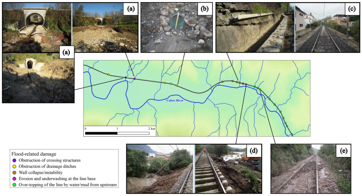
Intense precipitation and the subsequent flooding caused widespread damage to the railway line and led to six days of service disruption. Damage resulted primarily from: (i) overflowing of the Calore River, (ii) interaction with surface runoff, and (iii) significant sediment transport, resulting in overflow, erosion, and debris accumulation at the intersection between the railway line and the secondary right-bank Calore River tributaries. The consequences of these phenomena included instability of retaining walls and railway embankments, obstruction of drainage facilities, and debris material accumulation adjacent to crossing structures (culverts and bridges). In most cases, the recorded damage could not be attributed to a single mechanism but rather a combination of multiple geohydraulic factors. Figure 2 shows the approximate location and typology of the damage recorded along the railway after the storm, provided by the railway company. The main damage caused by the event is summarized in Table 1.

3. Methodology

In this section, we present a six-stage stepwise process for creating flood susceptibility maps and define the contributing flood-influencing factors.

3.1. Methodology Flowchart

We apply a GIS-based multi-criteria approach for the flood susceptibility assessment of the railway track described in Section 2. The AHP was selected as the factors’ weighting method within the framework of MCA. The numerical codes used in this work were in the open-source GIS environment QGIS (version 3.28.3), to create, process, and analyze geospatial data, and the Microsoft Excel (version 2408) spreadsheet environment for the AHP application. The study is based on the following main six stages (Figure 3):
-
The data required for the analysis were collected from various sources and pre-processed in GIS.
-
Several flood-influencing factors (FIFs) covering hydrological, geomorphological, environmental, topographical, and meteorological conditions, based on the actual characteristics of the study area, were selected. Input data for each factor were resampled in the GIS environment as raster data with 10 m spatial resolution, resulting in 4,306,822 cells (2194 columns, 1963 rows), and reprojected in the reference system WGS 84/UTM zone 32 N. We classify the FIFs into seven static flood-conditioning factors (FCFs: elevation, slope, topographic wetness index, distance to streams, drainage density, land use/land cover and geology) and one dynamic flood-triggering factor (FTF, October 2015 rainfall). Due to the diverse nature of each factor, all the thematic maps were reclassified on a scale from 1 to 5 (rating score), where 1 refers to a very low (or negligible) level of influence/susceptibility to flooding and 5 to a very high level. The approach of setting a priori the number of susceptibility classes is also employed in similar studies for identifying flood-prone areas [38,42,56,60,70,71,72,73].
-
The AHP technique was employed to determine the relative weights of the flood-influencing factors.
-
The thematic map layers were superposed in GIS using the weights calculated with the AHP technique. A flood susceptibility condition map (FSC) was created by combining the seven FCFs with their weights, and a flood susceptibility assessment map (FSA) was obtained by combining the seven FCFs and the one FTF (rainfall) with their weights. The pixel value of each output map (FSi) was obtained using the following equation (weighted linear combination, WLC, [74]):
F S i = j = 1 n r i j w j
where n is the number of factors, rij is the rating score (from 1 to 5) of the j-th factor at each grid cell i, and wj is the weight of the j-th factor calculated with the AHP method.
-
A sensitivity analysis was applied to both the FSC and FSA maps to evaluate the influence of uncertainties of the input factors’ weights on the derived flood susceptibility maps.
-
To validate the flood susceptibility zonation method, historical flood-related damage sites on the railway infrastructure from the railway company and official flood inundation maps from the competent authorities were used.

3.2. Flood-Influencing Factors (FIFs)

The primary challenge for any flood susceptibility assessment is to identify a set of appropriate influencing factors based on the actual geomorphological and hydrological conditions of the study area [60]. To avoid unreliable weights dominated by one predominant factor, it is generally recommended to consider at least six conditioning factors in the evaluation of areas susceptible to flooding [38,60]. These factors were selected based on an extensive literature review [31,38,39,41,42,44,45,49,50,51,52,53,54,55,58,60,70,72].
For all the numerical factors (except distance from the drainage network), the Jenks natural breaks classification method [75] was applied (with appropriate Python code) to establish different flood susceptibility levels [41,42,44,70,71]. The qualitative parameters of land use/land cover and geologic formations were classified according to the characteristics of the study area [63].
Although not exhaustive, the cited factors offer a comprehensive representation of the major influential variables that may impact flood occurrence within the study area. In the following, we provide an overview of source data and processing related to the selected FIFs.

3.2.1. Elevation (E)

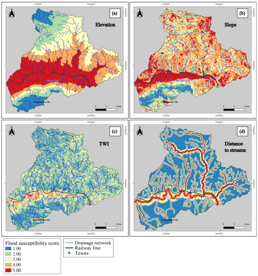
Topographic elevation is commonly used in assessing flood-prone areas, as lowland regions are generally more susceptible to floods [39,43]. The high level of susceptibility connected to lowlands arises from the natural flow of water from higher to lower elevation points. For each cell, the elevation values were obtained from the digital elevation model (DEM). A freely accessible DEM with a spatial resolution of 10 m, produced by the National Institute of Geophysics and Vulcanology (INGV) for the whole Italian territory, was downloaded from https://tinitaly.pi.ingv.it/ in February 2023 [76]. The elevation of the study area varies from 47 m a.s.l. to 1385 m a.s.l. and was divided into five classes (Figure 4a and Table 2): the lowest elevation class was allocated a value of 5 (very high susceptibility to flooding) and a score of 1 (very low susceptibility) was attributed to the highest elevation category. The elevation map (Figure 4a) shows that the highest susceptibility scores are in the flat area characterizing the Low Calore River alluvial floodplain.

3.2.2. Slope Angle (S)

Slope, defined as the tangent of the angle β between the Earth’s surface and a horizontal reference [77], plays a fundamental role in hydrology and geomorphology. It influences the movement of water and materials under gravity, impacting various processes such as soil water content, erosion, geomorphic evolution, and flood dynamics [33,78]. In simplified terms, for a given flow rate at a specific point, a decrease in the local slope will lead to an increase in water depth (and a corresponding decrease in flow velocity), and vice versa. Consequently, areas with gentle slopes are prone to water accumulation and stagnation, making them susceptible to flooding. For each cell, the slope angle was derived from the DEM using the slope function available in QGIS. The study area, a steeply sloping terrain where the slope angle ranges from 0° to 70.8°, was divided into five classes (Figure 4b and Table 2): the lowest slope category was allocated a score of 5 (very high susceptibility), while the highest slope category was given a value of 1 (very low susceptibility to flooding). From Figure 4b we note that the southern part of the catchment is dominated by the steep slopes of Mount Camposauro, while the central part is dominated by the flat Calore River floodplain.

3.2.3. Topographic Wetness Index (TWI)

The topographic wetness index (TWI) represents the potential for water to accumulate at any point within the drainage basin and to move downslope driven by gravitational forces [78]. It is computed with the TWI algorithm from SAGA Next Gen in QGIS as ln(a/tanβ), where a is the upslope area draining through a certain point per unit contour length (m2 m−1) and tanβ is the local slope where β is expressed in radians [79,80,81]. The catchment area a represents the upstream drainage area per unit contour length expected to supply water to the pixel for which the TWI calculation is made. Since rainfall direction is assumed approximately vertical, the catchment area a is proportional to the flow rate passing through a point. Regions with large contributing drainage areas and gentle slopes will exhibit high TWI values, whereas small areas with steep slopes will correspond to low TWI values. In the study area, the TWI varies from 5.56 to 23.62 and was divided into five classes (Figure 4c and Table 2), with the highest values given the highest susceptibility score.

3.2.4. Distance to Streams (DS)

In addition to overland flows, river overflows play a pivotal role in triggering flood events, typically originating from the riverbed and extending into the surrounding areas. Thus, the proximity to rivers and streams significantly influences the susceptibility to flooding during such hazardous events. The river network map for the study area was retrieved from the National Summary Database (Database di Sintesi Nazionale, DBSN), freely downloaded (upon registration) from the Italian Military Geographic Institute (IGM) website (https://www.igmi.org/it/dbsn-database-di-sintesi-nazionale, accessed on 4 April 2023). The streams were classified using Strahler’s order system [82]. The main watercourse of the drainage network (the Calore River) is a fifth-order stream in the context of the study area. The distance to rivers was computed in QGIS using the Euclidean distance to the closest channel stream. Classes were created around first- and second-order streams at distances of 25, 50, 100, and 150 m, third-order streams at distances of 50, 100, 150, and 200 m, fourth-order streams at distances of 100, 200, 300, and 400 m, and fifth-order streams at distances of 100, 300, 500, and 700 m. The highest flood susceptibility score was assigned to the areas closest to the drainage network (Figure 4d and Table 2).

3.2.5. Drainage Density (DD)

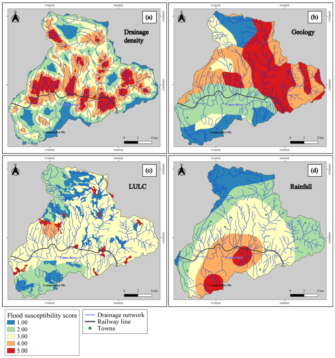
Drainage density is defined as the ratio of the total length of drainage channels per basin area [38,83]. Impermeable soils produce higher runoff which causes more pronounced soil erosion and an increase in drainage density [60]. The line density module in QGIS was applied. Figure 5a shows the drainage density map of the study area, obtained from the river network, which varies from 2.37–3.64 km/km2 (very high susceptibility to flooding) to 0–0.75 km/km2 (very low susceptibility), as reported in Table 2.

3.2.6. Geology (G)

The geology of an area may significantly affect flooding occurrences. Porous formations, such as coarse sand and aggregates, facilitate rainwater infiltration, while impermeable deposits consisting of marl and clays promote surface runoff. Permeable formations are often connected to alluvial sediments in lowlands, allowing the floodplain delineation. The geological formations in the study area were derived from the Italian geology map, freely downloaded from the National Geoportal (https://gn.mase.gov.it/portale/home, accessed on 20 June 2023). The soil types present in the study area are clay, sandstone and arenaceous marl, marl and calcareous marl, alluvial deposits, and limestone (Figure 5b and Table 2). Clay soils are characterized by very low permeability and so they constitute zones of very high susceptibility to flooding, while limestone soils, usually characterized by high permeability rates, have low susceptibility.

3.2.7. Land Use Land Cover (LULC)

The extent and nature of land use and land cover can influence the vegetation density, which in turn regulates both precipitation absorption and surface runoff rates. Consequently, dense vegetation areas may mitigate the flood hazard, while barren and sparsely vegetated areas may experience increased surface runoff and may be more susceptible to flooding.
The Corine land cover database (European Environmental Agency—EEA, http://www.eea.europa.eu, accessed on 21 June 2023) was used to identify the land uses of the considered catchment area. The land use/land cover types present in the study area are urban areas, sparse urban areas, agricultural lands (mostly dominated by vineyards and olive groves, [63]), grasslands and shrubs, and forests (mainly concentrated on the steepest slopes, [63]) (Figure 5c and Table 2). The highest susceptibility score was assigned to the urban areas.

3.2.8. Cumulative Two-Day Rainfall (C2DR)

In this study, rainfall was considered a dynamic triggering factor for flooding (flood-triggering factor, FTF) instead of a static conditioning factor [22]. Generally, high-intensity and long-duration rainfall correlates with increased overland flow and water runoff, affecting the magnitude of flooding phenomena.
For the historical event of autumn 2015, cumulative two-day rainfall (C2DR) was derived from the sub-hourly precipitation records of 30 hydrometeorological stations located inside and near the catchment area (21 stations managed by the regional Civil Protection Department—7 of which are auxiliary stations not used for civil protection activities—and 9 stations managed by the Regional Agrometeorological Service) from October 14th (20:00 h) to 15th (13:00 h), 2015. The inverse distance weighted (IDW) function in QGIS was used to determine the spatial distribution of rainfall. The rainfall spatial distribution varies from 77.5 mm to 305.1 mm and is divided into five classes (Figure 5d and Table 2). The greatest susceptibility was attributed to the highest precipitation class. The precipitation map (Figure 5d) shows that the highest precipitation values are mainly concentrated in the central and southern areas of the domain.

3.3. Calculation of Weights

A flood susceptibility condition (FSC) map was created by combining the seven FCFs with their weights, and a flood susceptibility assessment (FSA) map was obtained by combining the seven FCFs and the one FTF (rainfall) with their weights. According to the factors’ relevance for the occurrence of flood phenomena, the weight values were determined with the analytic hierarchy process (AHP).
The AHP is a multi-criteria method that has been widely employed in various decision-making applications [84]. The procedure estimates criteria weights through pairwise comparisons using numerical importance scales [85,86], offering a structured approach for evaluating and integrating the effects of various factors within the framework of natural hazard and risk management [87].
The application of the procedure involved five experts who were part of the study (three from the academy and two from the railway industry). The most relevant factors to include in the analysis were derived from the literature and discussed during group settings, adding relevant factors that were first neglected or removing irrelevant ones. Pairwise judgments were administered through surveys and interviews during online group sessions, using a scale of relative importance between factors [85] that ranges from one (equal importance) to nine (extreme importance). During the first step, pairwise judgments were expressed among the seven FCFs. The correspondent pairwise comparison matrix obtained from the experts’ opinions was normalized with the principal eigenvector method, obtaining the relative weights of the seven factors (see Table 3, third column), and subsequently evaluated for consistency. This process is described in Appendix A.
During the second step, eight factors (the seven FCFs plus the triggering rainfall) were considered: the pairwise judgments from the previous step were retained and the experts were called to express their opinions on the importance of the triggering rainfall. Again, the correspondent pairwise comparison matrix was normalized and tested for consistency. Table 3 (fourth column) shows, for each factor, the final relative weight, which represents its expected contribution to the occurrence of flood phenomena in the considered research area.
During the first step, slope and distance to streams emerged as the most significant factors for flood occurrence, while geology and LULC were considered the least influential (Table 3, third column). In the second step, the rainfall spatial distribution was the most influential factor (Table 3, fourth column) for the construction of the flood susceptibility assessment map. The weights assigned to the various factors are not fixed and may be reviewed and updated regularly.

4. Map Interpolation and Sensitivity Analysis

The proposed methodology integrates the selected flood-influencing factors through a linear combination, considering the relative weights calculated with the AHP method (Section 3.3 and Appendix A). This process entails overlaying the thematic maps of Figure 4 and Figure 5 with different weights in QGIS through the weighted linear combination (WLC) of Equation (1) (using the Raster Calculator).
A flood susceptibility condition map (FSC) was created by combining in QGIS the seven flood-conditioning factors with their weights (Table 3, third column):
F S C = 0.255 × S l o p e + 0.255 × D i s t a n c e f r o m s t r e a m s + 0.151 × T W I + 0.151 × E l e v a t i o n + + 0.092 × D r a i n a g e D e n s i t y + 0.058 × G e o l o g y + 0.039 × L a n d U s e L a n d C o v e r
and a flood susceptibility assessment (FSA) map was obtained by combining the seven flood-conditioning factors and the one flood-triggering factor (rainfall) with their weights (Table 3, fourth column):
F S A = 0.219 × R a i n f a l l + 0.201 × S l o p e + 0.201 × D i s t a n c e f r o m s t r e a m s + 0.116 × T W I + + 0.116 × E l e v a t i o n + 0.069 × D r a i n a g e D e n s i t y + 0.045 × G e o l o g y + + 0.031 × L a n d U s e L a n d C o v e r
These maps provide the spatial variability of flood susceptibility within the entire study area. Finally, flood-prone areas were split into five susceptibility classes (“very low”, “low”, “moderate”, “high”, and “very high”) using the Jenks breaks classification (with a custom Python script).

Sensitivity Analysis

Variability of the selected factors may introduce biases into the susceptibility assessment process. An investigation was conducted to examine the impact of uncertainty in the assigned factor weights on the flood susceptibility assessment. At each cell grid, the error Δεi produced by the uncertainties Δwj of the weighting coefficient values wj is [49,50,88,89]:
Δ ε i = j = 1 n Δ w j r i j 2
where n is the number of factors and rij is the rating score (from 1 to 5) of the j-th factor at each grid cell i. The factor weights wj used for the basic FSC map (see Table 3) were altered by 20% with respect to their original values. The changes in weight values (Δwj) of every factor are: 0.051 for slope, 0.051 for distance to streams, 0.0301 for TWI, 0.0301 for elevation, 0.0183 for drainage density, 0.0117 for geology, 0.0078 for LULC. This procedure led to the creation of a map (representing the error Δεi at each grid cell) that was added and subtracted from the basic FSC map to represent two extreme scenarios of maximum and minimum values (FSCmax and FSCmin, respectively). The same procedure was repeated for the basic FSA map—with the changes in weight values of 0.0437 for rainfall, 0.0402 for slope, 0.0402 for distance to streams, 0.0233 for TWI, 0.0233 for elevation, 0.0139 for drainage density, 0.0091 for geology, 0.0063 for LULC—obtaining two extreme scenarios of maximum and minimum values (FSAmax and FSAmin, respectively). Thus, a total of six maps were obtained.

5. Results and Discussion

This section presents the findings of investigations into spatial variations of flood susceptibility across the study area and subsequent validation.

5.1. Spatial Variation of Flood Susceptibility at Basin Level

The spatial distribution of the flood susceptibility obtained with the AHP weights and WLC method implemented in QGIS has been created (Figure 6 and Figure 7). Susceptibility was split into five classes (“very low/negligible”, “low”, “moderate”, “high”, and “very high”) using the Jenks breaks classification method (with a custom Python script).
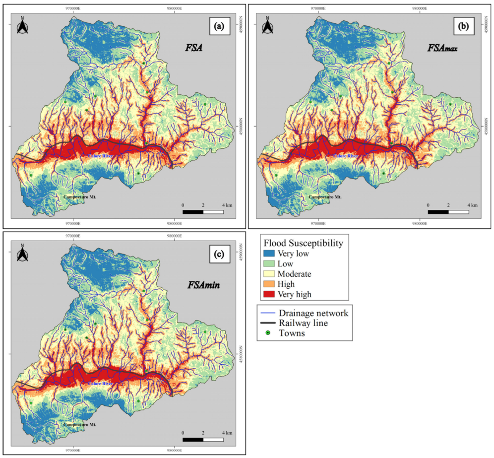
Figure 6a illustrates the basic FSC map along with the upper (FSCmax, Figure 6b) and lower (FSCmin, Figure 6c) values, derived by accounting for the uncertainty in the factors’ weights (see Section 4). The basic FSC map reflects the influence of the seven static FCFs (elevation, slope, topographic wetness index, distance to streams, drainage density, land use/land cover and geology) on the occurrence of flood phenomena in the study area, and the two additional maps (FSCmax and FSCmin) account for the uncertainties in the weights of the adopted factors.
Figure 6a shows that the flood-prone areas (with “high” and “very high” flood susceptibility) are mainly located in the low-lying Calore River floodplain and along its tributary streams. As also reported by several studies [41,43,44], the most susceptible areas to flood generally present a common pattern of very low altitude, low slope angle, high drainage density, and proximity to streams. The junctions of low-order streams with the main watercourse represent areas with “very high” flood susceptibility. In contrast, the susceptibility is “negligible” in the higher-elevation and steeper slope zones at the foot of the Mt. Camposauro northern face (southern part of the domain). These areas, which are entirely covered by forests and grasslands, are characterized by very low to moderate drainage density values, and low TWI values, and mainly comprise limestone formations (with high permeability). Similarly, the northern part of the domain is characterized by higher elevation and moderate/low slope degree areas with established vegetation cover and permeable geological formations and consequently flood susceptibility ranges from “very low” to “moderate”.
Figure 7a illustrates the basic FSA map for the storm event together with the upper (FSAmax, Figure 7b) and lower (FSAmin, Figure 7c) scenarios, derived by considering uncertainty in factor weightings (see Sec. 4). The basic FSA map reflects the combined effect of the seven FCFs and the one FTF (cumulative two-day rainfall) on the flooding event that occurred in the study area.
The FSA map shows those areas located along the main watercourse and its tributary streams expected to have “high” and “very high” flood susceptibility due to the combination of intense precipitation with low-lying topography, gentle slope, high drainage density, and proximity to streams. In particular, the regions with the highest susceptibility are mainly concentrated in the central part of the study area (encompassing the Low Calore River floodplain, the regions along its low-order tributaries, and the slopes above rivers and rivulets), which is most affected by high-intensity rainfall. This agrees with the general picture of the effects produced on the territory by the extreme meteorological event, i.e., fluvial flooding, and hillslope processes (soil erosion, debris flow, earth flow) [68]. In contrast, in the northern part of the catchment, large areas are characterized by “negligible” susceptibility because of scarce intensity precipitation combined with higher altitude, moderate to low slope angle, low drainage density, extensive vegetation cover, and permeable geological formations.
In both flood susceptibility zonation maps, “very high” and “high” susceptibility zones mostly cover the areas along and near the rivers [43]. The highest flood potential regions also cover the areas along the streams’ junctions, proving that the drainage density is an important contributor to flooding. On the other hand, the lowest flood potential areas are distributed in the more elevated and steeper areas from where the runoff water rapidly propagates to the low-lying regions encompassing the Low Calore River alluvial floodplain [41].
The percentages of the susceptibility classes, concerning the entire catchment area, are given in Table 4. Notably, the basic FSC map classifies about 66.5% of the study area with “very high” to “moderate” flood susceptibility and 33.6% as comprising “low” and “very low” susceptibility zones. This implies that a large proportion of the catchment is susceptible to flooding as a function of the region’s intrinsic characteristics. Similarly, the basic FSA map classifies about 64.8% of the study area with “very high” to “moderate” flood susceptibility levels and 35% as “low” and “very low” susceptibility zones (Table 4). This implies that considering the event rainfall does not increase the percentage area of the highest susceptibility, but rather leads to a spatial redistribution of susceptibility classes within the catchment area.
From Table 4 it is observed that, regarding the FSCmax map showing the upper susceptibility values relative to the basic FSC map, the spatial extent of the “moderate” and “negligible” susceptibility classes has decreased, the extent of the “high” and “very high” susceptibility zones has increased, while the percentage area of “low” susceptibility has remained unchanged. For the FSCmin map showing the extreme scenario of minimum susceptibility values, the areas of “moderate” and “low” susceptibility classes have decreased, the extent of the “high” and “very high” susceptibility zones has increased, while the percentage area of “very low” susceptibility has remained constant. Therefore, both the FSCmax and FSCmin maps are characterized by an increase in the “high” and “very high” susceptibility zones and a decrease in the “moderate” susceptibility zones relative to the basic FSC map (Table 4). Compared with the basic FSA map, the spatial extent of the “high” and “very high” susceptibility classes in the FSAmax map has decreased, while the extent of the “negligible”, “low”, and “moderate” classes has increased. For the FSAmin map, the areas of the “low”, “moderate”, “high”, and “very high” classes have decreased, whereas only the spatial extent of the “negligible” susceptibility has increased. The FSAmax and FSAmin maps share a decrease in “high” and “very high” zones and an increase in “very low” susceptibility zones, relative to the basic FSA map. In summary, the four additional maps that account for the uncertainty in the factors’ weights (FSCmax and FSCmin, and FSAmax and FSAmin) present no significant differences in the spatial distribution of susceptibility relative to the basic FSC map and FSA map, respectively, demonstrating the robustness of scoring and the model outcomes.
Figure 8 shows the spatial distribution of the absolute difference between the FSC map of Figure 6a and the FSA map of Figure 7a for the study area. The main difference between the two maps (red) can be found in the southern part of the study area, at the foot of the Mt. Camposauro northern slope, due to the strong influence exerted by the rainfall intensity (as flood-triggering factor) in the FSA map of Figure 7a. The southern part of the catchment is mainly classified with a “very low” susceptibility (blue) in the FSC map (Figure 6a), while large portions with “low” susceptibility (green) appear, for the same area, in the FSA map (Figure 7a).

5.2. Impact of Factors on the Flood Susceptibility Distribution

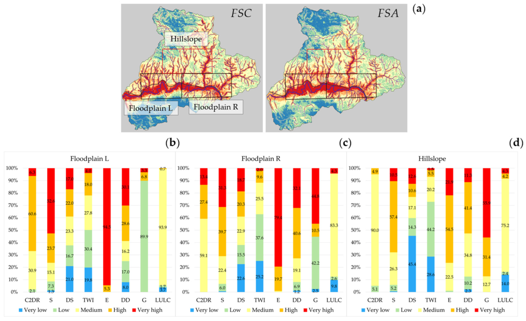
Figure 9 illustrates the percentage distribution of the influence/susceptibility levels (low, very low, medium, high, very high) of the eight factors (that contributed to constructing the flood susceptibility maps, the FSC map of Figure 6a and the FSA map of Figure 7a) across different regions of the domain. Specifically, two regions were considered (Figure 9a): (i) the floodplain, which was further divided into the left (Floodplain L) and right (Floodplain R) zones, and (ii) a portion of the hillslope located immediately north of the floodplain (Hillslope). On the x-axis, the influencing factors are ordered from left to right according to the importance assigned to them by the experts, based on the weights determined using the AHP method (Table 3). The inspection of the figure shows the variable impact of the different factors in the regions considered. Clearly, the higher the percentage of “high” and “very high” influence/susceptibility levels, the greater the impact of a single factor on the flood susceptibility of a specific area (regardless of the AHP weights assigned to the various factors).
In the left part of the floodplain (Figure 9b), the highest rainfall exerts a dominant influence, along with very gentle slopes, low elevation, and high drainage density. There is also a notable influence from the short distance to streams and the high TWI driven by the large upstream drainage area and gentle slopes. In conclusion, the flood susceptibility of this floodplain area is primarily determined by its geomorphology, characterized by very low elevations, flat terrain, a large upstream drainage area, the dominance of the Calore River, and a dense network of secondary tributaries on the right hydraulic side. The autumn 2015 storm event negatively impacted the already highly susceptible context.
Conversely, in the right part of the floodplain (Figure 9c), the drainage network density is higher than in the left part (due to the presence of numerous secondary tributaries on both the right and left hydraulic sides of the main watercourse), and geology plays a more significant role, as the more impermeable clay and sandy formations have markedly increased. Land use and land cover (LULC) also have a greater influence on overall flood susceptibility, due to the presence of urbanized and/or industrial impervious areas. For this reason, the right part of the floodplain is also highly susceptible to flooding due to its geomorphology, and the presence of highly impermeable geological formations further contributes to this susceptibility. The rainfall event considered has also negatively impacted this area, already highly susceptible to flooding.
The situation differs, however, in the hillslope area located immediately north of the floodplain (Figure 9d). Here, the highest rainfall has limited importance, close distance to streams and high drainage density continue to exert some influence, while the influence of geology on flood susceptibility increases significantly due to the extensive presence of highly impermeable geological formations. In conclusion, flood susceptibility of the hillslope region is primarily concentrated in areas along the low-order tributaries of the main Calore River, being influenced by the presence of impermeable geological formations.

5.3. Validation of the Methodology

Validation ensures that the procedure requirements are fulfilled [90,91]. Figure 10 shows the spatial distribution of flood susceptibility in the area surrounding the railway track, derived from the basic FSC map of Figure 6a (Figure 10a,b) and the basic FSA map of Figure 7a (Figure 10c,d), respectively. Figure 10 also shows the approximate position of 22 flood-related damage sites recorded along the railway infrastructure after the October 2015 storm event, which are marked with circular points and numbered from 1 to 22 (see Section 2 and Figure 2). To verify the flood susceptibility zonation model, the two outcome maps developed (the FSC map of Figure 10a,b and the FSA map of Figure 10c,d), were compared against the flood-related damage sites along the railway. As shown in Figure 10b and Table 5, 21 disasters (numbers 1 to 5 and 7 to 22) occurred in the areas of “very high” susceptibility, while disaster number 6 occurred in the “high” susceptibility area. According to the FSA susceptibility zonation (Figure 10d and Table 5), 21 disasters (numbers 1 to 18 and 20–22) occurred in the areas of “very high” susceptibility, while disaster number 19 occurred in the “high” susceptibility area. The sensitivity analysis shows that weighting uncertainty does not impact this outcome. All flood-induced damage was found to occur in the “very high” or “high” susceptibility zone (Table 5), demonstrating a close relationship between modeled and real-world hazards. This also suggests that the flood susceptibility condition (FSC) map (exclusively based on static factors) is as suitable as the flood susceptibility assessment (FSA) map, which includes the dynamic aspect of event rainfall.
The flood susceptibility zonation model was verified by comparison with the inundation maps available from the relevant authorities. In Italy, seven River Basin District Authorities (RBDAs) produce flood inundation hazard maps according to the European Floods Directive 2007/60/EC [92]. These maps delineate the areas that could be potentially affected by riverine flood events for three different hazardous scenarios: (i) low probability hazard (LPH) for rare events (with return period, also called recurrence interval, ranging in the interval T = 200–500 years), (ii) medium probability hazard (MPH) for frequent events (with T = 100–200 years), and (iii) high probability hazard (HPH) for very frequent events (with T = 20–50 years). The maps from different basin authorities were merged into one map covering Italy by the Italian Institute for Environmental Protection and Research (ISPRA). The national coverage map was last updated in 2021 [13] and is freely available from the ISPRA website (https://idrogeo.isprambiente.it/app/page/open-data, accessed on 17 November 2022) in vector polygon format.
In many areas of the Italian peninsula, official flood hazard maps are absent or incomplete since low-order streams are generally omitted [15], and non-fluvial flood phenomena like pluvial/surface flooding are not properly accounted for. Figure 10 shows the overlap between the official fluvial flood hazard map with MPH (with T = 100 years) and the railway track. In the study area, the official flood inundation extent for the MPH was determined by the competent authority using a combination of numerical hydraulic simulations of the Calore River overflow, which were available before the autumn 2015 event, and surveys that included multiple in situ assessments conducted by technicians to document the areas affected by the Calore River overflow during the autumn 2015 storm event (the details are available from the RBDA website: https://www.distrettoappenninomeridionale.it/, accessed on 17 November 2022).
The official fluvial flood hazard map does not perfectly overlap in the GIS environment with the locations of the damage to the railway infrastructure (Figure 10 and Table 5). This is partly expected since the official flood hazard map does not directly account for the overflows of low-order Calore River tributaries and surface runoff water processes on hillslopes. Therefore, disasters 3–6 (related to the clogging of drainage facilities) and disasters 13–22 (related to the obscuring of railway segments), both attributed to sediment and debris materials transported by overland flow and secondary tributaries, could not be adequately anticipated from the official fluvial flood hazard map despite the updates made based on post-event surveys following the autumn 2015 storm event.
The proposed flood susceptibility zonation can identify not only the segments of railway infrastructure intersecting with flood-prone areas but also potential infrastructural damage sources, attributed to the effect of direct rainfall, which are currently not incorporated into the official flood hazard maps from the RBDAs. Further, the modeled flood susceptibility zonation shows a significant correspondence between the flood-prone areas and the spatial occurrence of flood-related incidents on the railway. Thus, the validation process substantiates the reliability and accuracy of the generated maps. The FSC map proves to be sufficiently accurate for identifying areas susceptible to flood along the railway compared to the FSA map, despite not accounting for the precipitation within the watershed during the considered event.
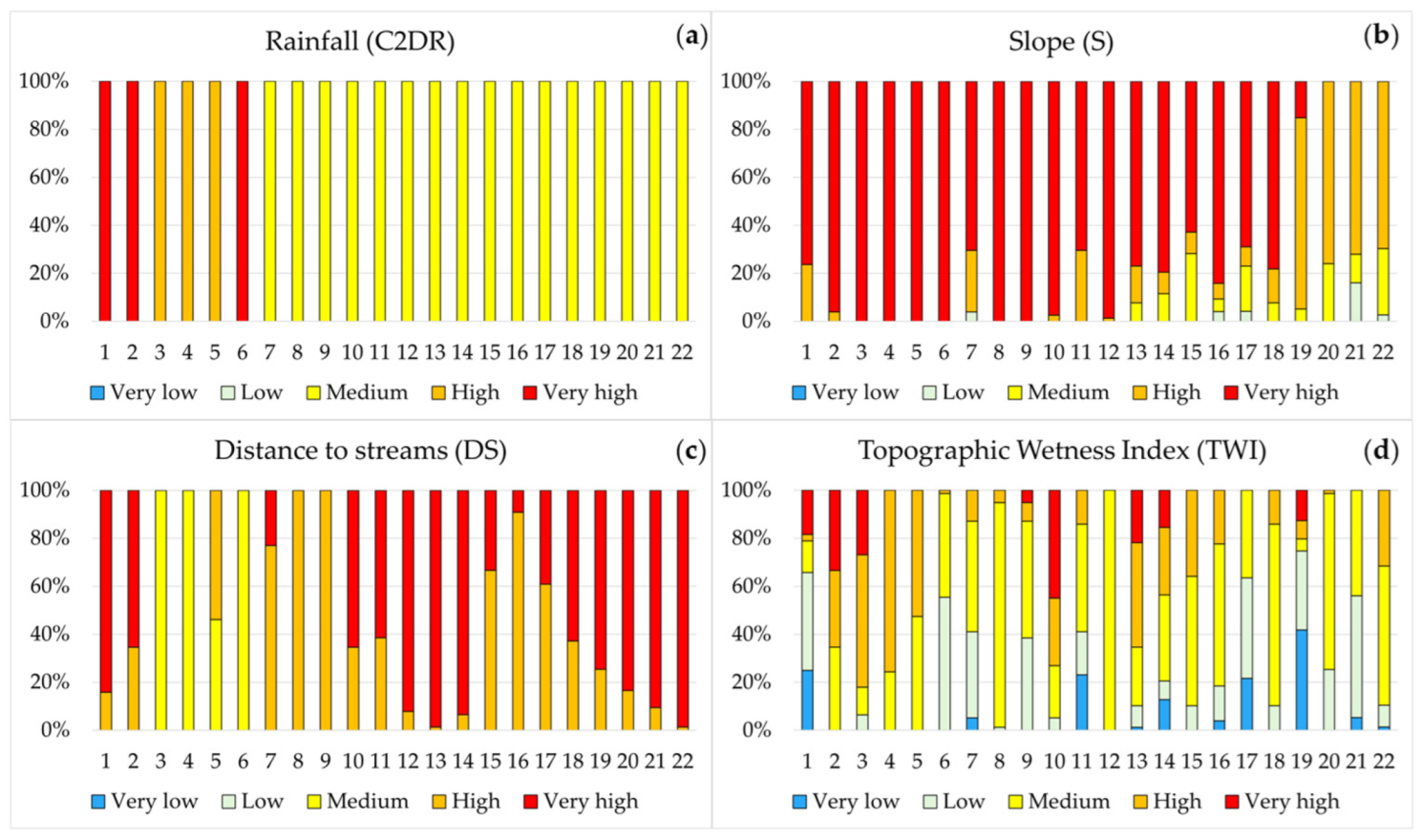
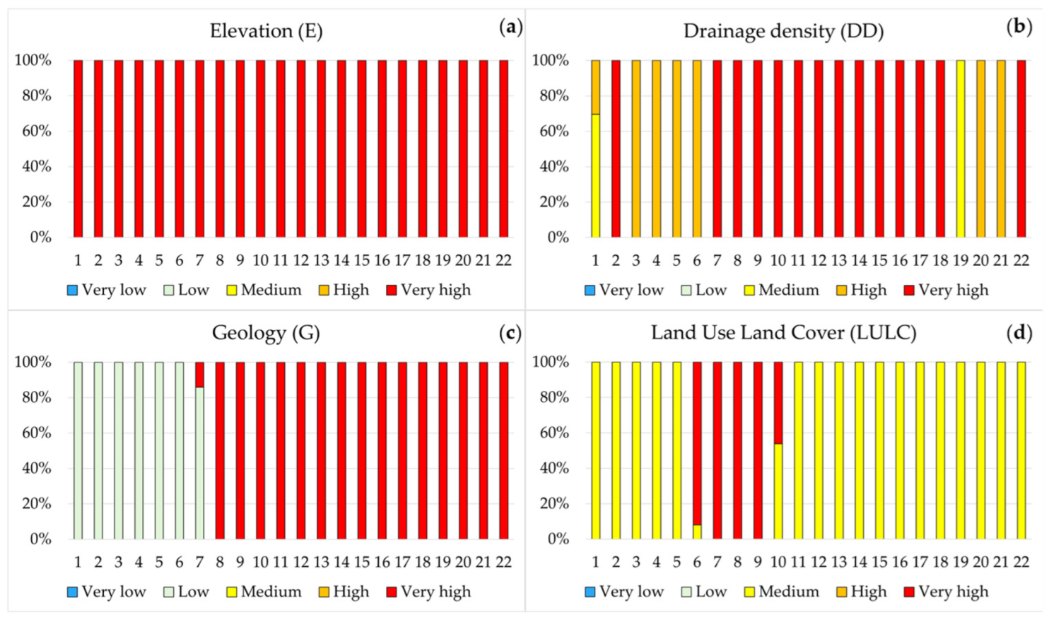
In the GIS environment, a circle with a radius of 50 m was drawn around each damage site, and the percentage of influence/susceptibility level for each factor was evaluated relative to these circular areas. Figure 11 and Figure 12 illustrate the percentage distribution of influence/susceptibility levels (low, very low, medium, high, very high) of the eight flood-influencing factors across the 22 recorded damage sites (x-axis). By analyzing the figures, it is evident that all damage occurred in areas with the lowest elevation and slope. Most of the damage also appears to have been influenced by the high drainage network density and proximity to streams. The damage most influenced by rainfall occurred west of the town of Ponte (Figure 11a, damage sites 1–6), while that most affected by geology was located within and to the east of the town (Figure 12c, damage sites 8–22).

5.4. Limitations and Future Research Directions

The proposed methodology provides a comprehensive framework for identifying areas and rail infrastructure that may be susceptible to flood events. However, potential limitations should be considered:
-
The inherent subjectivity in expert assessments within the analytic hierarchy process (AHP) can lead to biases in the weighting of criteria, even though pairwise comparisons are used to promote consistency. The influence of this bias can be assessed with sensitivity analysis conducted on weights.
-
The accuracy and resolution of the input data could introduce uncertainties, particularly in regions with complex topography or diverse land cover. Depending on the scope of the susceptibility map, different scales could be required for different applications.
-
The present application considers the rainfall forcing from the 2015 autumn event only. There is the potential to include present climate (rainfalls with different durations and intensity) and future projections where available.
-
The extent and nature of present land use and land cover (LULC) do not account for historical modifications or predict future changes. Future developments of the territory should be included if the corresponding information is available.
Considering these limitations, future research could broaden the analysis by integrating additional factors, including socio-economic aspects and the physical vulnerability of the infrastructure. The procedure could also account for the spatial variability of rainfall over extended time periods, potentially incorporating future changes due to climate change. Additionally, the methodology could be adopted for application to other types of transportation infrastructure networks, particularly roads, and at broader scales, such as regional or national levels.

6. Conclusions

This study has considered a GIS-based multi-criteria approach (based on catchment descriptors and rainfall forcing) to create rapid prediction maps of flooding-susceptible areas along railway lines. The importance of the study stems from a gap in implementing GIS-based MCA techniques for flood susceptibility mapping along rail infrastructure that consider multiple flood sources (e.g., heavy rainfall and river flooding). The procedure, which could also be applied to other types of linear transport infrastructures in flood-prone regions, has been demonstrated using a case-study rail track in southern Italy that was affected by a destructive flood in the autumn of 2015.
Two susceptibility maps were produced, with one excluding the 2015 event rainfall forcing. The findings highlight that large portions of the case-study railway intersect with areas characterized by high flood susceptibility, based on the physical characteristics of the region. The most critical zones cover the areas close to and along the main river, its low-order tributaries, and the streams’ junctions. The inclusion of rainfall as a triggering factor leads to a redistribution of the highest-flood-susceptibility areas, mainly concentrated in the central part of the catchment.
The flood susceptibility maps correlate well with recorded post-event flood-related damage along the railway, whilst the official fluvial flood inundation maps fail to supply information about flooding occurring along secondary tributaries and from direct rainfall. The proposed zonation highlighted the importance of secondary tributaries and rivulets in flood occurrence in the study area, underscoring their necessity for inclusion in flood hazard assessments from railway and environmental authorities. This provides a worthy insight into the correlation between flood sources and railway damage, prompting the adjournment of the official flood inundation maps that do not consider the effect of pluvial/surface flooding.
From the validation, the flood map excluding triggering rainfall is sufficiently accurate for identifying flood-prone areas along the rail route. This may have important practical implications since the construction of this map relies on a small set of readily available data.
The main limit of the proposed methodology is that the outcome, i.e., the zonation of the flood susceptibility areas, is dependent on expert judgements and, thus, could suffer from sensitivity to changes (i) in the selection of the factors and (ii) in the weights assigned to the adopted factors. Despite their subjectivity, the obtained flood susceptibility maps may provide railway (and environmental) authorities with the reliable spatial distribution of flood-critical locations for limiting infrastructural damage and service disruptions. This information could be used to prioritize future targeted investments of more detailed analysis, to carry out targeted preventive measures (maintenance of drainage pipes, culverts, and ditches susceptible to debris clogging and maintenance of gullies to avoid obstruction from vegetation), and to implement flooding early warning systems by individuating appropriate locations for the deployment of real-time rainfall gauge stations. The study also reinforces the importance of promptly recording infrastructural damage data to improve the analysis of hazard–impact relations on the railway in the post-disaster phase.
The proposed methodology may offer railway authorities a cost-effective strategy for protecting infrastructure assets in the long term, aiding in decision making and maintaining operational rail routes. This is crucial for minimizing operational risk and mitigating the socio-economic impacts of flooding at regional and national levels.

Author Contributions

G.V.: Conceptualization (lead), Methodology (lead), Formal analysis (lead), Investigation (lead), Data curation (lead), Software (lead), Writing—original draft (lead), Writing—review and editing (equal), Visualization (lead). R.D.M.: Writing—original draft (supporting), Writing—review and editing (supporting), Supervision (supporting). M.T.: Writing—original draft (supporting), Supervision (supporting). A.F.: Writing—original draft (supporting). A.Z.: Writing—original draft (supporting). I.A.: Writing—original draft. C.A.B.: Writing—original draft (supporting), Writing—review and editing (equal). N.Q.: Writing—original draft (supporting), Writing—review and editing (equal). J.E.L.: Writing—original draft (supporting), Writing—review and editing (equal), Supervision (supporting). L.C.: Writing—original draft (supporting), Writing—review and editing (equal), Supervision (lead). All authors have read and agreed to the published version of the manuscript.

Funding

This research was co-funded by the European Union program FSE-REACT-EU, PON Ricerca e Innovazione 2014–2020 DM1062/2021 (Grant No. CUP-I65F21001120001).

Data Availability Statement

Most data used in this study are from publicly sourced databases available at the sources included in the article. Restrictions apply to the availability of data concerning flood-related damages along the railway due to privacy and security issues. The original contributions presented in the study are included in the article, further inquiries can be directed to the corresponding authors.

Acknowledgments

The lead author (GV) expresses her thanks for the co-funding provided by the European Union program FSE-REACT-EU, PON Ricerca e Innovazione 2014–2020 DM1062/2021. All the authors are grateful to Dr Anna Pelosi for kindly providing rainfall data to support the initial phases of the work. All the authors want to acknowledge the Editor and the Referees for their constructive comments that contributed to improving the manuscript’s original version.

Conflicts of Interest

The authors declare no conflict of interest.

Appendix A. Analytical Hierarchy Process (AHP)

Appendix A.1. Development of the Pairwise Comparison Matrix

Let us consider a finite set of criteria C = {C1, C2, …, Cn}, with n ≥ 2, that need to be ranked with reference to a certain goal. The paired comparison in terms of the relative importance of the criterion Ci over Cj is undertaken by the experts/raters using the semantic scale of Table A1 and is converted into a numerical integer value aij > 0 (i, j = 1, …, n).
Table A1. Saaty’s comparative scale [85].
Intensity of ImportanceValues for
Reciprocal Scale
Definition
11Equal importance
21/2Equal to moderate importance
31/3Moderate importance
41/4Moderate to strong importance
51/5Strong importance
61/6Strong to very strong importance
71/7Very strong importance
81/8Very to extremely strong importance
91/9Extreme importance
The relative importance of the criterion Cj over Ci is defined as its reciprocal. As a result of the pairwise comparison, a (n × n) positive reciprocal matrix A is created using the values aij (i, j = 1, …, n):
A = a 11 a 12 a 13 a 1 n a 21 a 22 a 23 a 2 n a 31 a 32 a 33 a 3 n a n 1 a n 2 a n 3 a n n ,   a i i = 1 ,   a j i = 1 a i j ,   a i j 0 .
Table A2 and Table A3 show the pairwise comparison matrix derived from the experts’ judgment for the first case in which only the seven flood-conditioning factors are considered (n = 7) and the second case in which the seven flood-conditioning factors and the one flood-triggering factor are considered (n = 8), respectively. After developing the pairwise comparison matrix, it is possible to calculate the factors’ weights.
Table A2. Pairwise comparison matrix: the seven Flood-Conditioning Factors are considered as criteria (n = 7).
Pairwise Comparison Matrix
FactorSDSTWIEDDGLULC
Slope (S)1122345
Distance from streams (DS)1122345
Topographic wetness index (TWI)1/21/211234
Elevation (E)1/21/211234
Drainage density (DD)1/31/31/21/2123
Geology (G)1/41/41/31/31/212
Land use land cover (LULC)1/51/51/41/41/31/21
Column sum3.783.787.087.0811.8317.524
Table A3. Pairwise comparison matrix: the seven Flood-Conditioning Factors and the one Flood-Triggering Factor are considered as criteria (n = 8).
Pairwise Comparison Matrix
FactorC2DRSDSTWIEDDGLULC
Rainfall (C2DR)11122456
Slope (S)11122345
Distance from streams (DS)11122345
Topographic wetness index (TWI)1/21/21/211234
Elevation (E)1/21/21/211234
Drainage density (DD)1/41/31/31/21/2123
Geology (G)1/51/41/41/31/31/212
Land use land cover (LULC)1/61/51/51/41/41/31/21
Column sum4.624.784.789.089.0815.8322.530

Appendix A.2. Normalized Pairwise Comparison Matrix and Computation of the Criteria Weights

The priority ranking vector, i.e., the vector of weights, w = (w1, w2, …, wn)T, with w1 > 0, …, wn > 0 and i = 1 n w i = 1 , can be estimated by means of the principal eigenvector method [93] solving the following equation:
A w = λ max w ,
where λmax is the largest eigenvalue in modulus of the matrix A. An easy way to approximate the priority vector w is to [93,94]:
-
sum the values in each column of the judgement matrix A (obtaining the column total, as shown in Table A2 and Table A3, respectively),
-
divide each element of the matrix A by its column total (obtaining the so-called normalized pairwise comparison matrix),
-
average over each row of the resulting normalized pairwise comparison matrix (i.e., divide the sum of the normalized elements of each row by the number of criteria n), thus obtaining an estimate of the criteria weights.
Table A4 and Table A5 show the normalized pairwise comparison matrix and the overall relative weights of criteria for the first case in which only the seven flood-conditioning factors are considered (n = 7) and the second case in which the seven flood-conditioning factors and the one flood-triggering factor are considered (n = 8), respectively.
Table A4. Normalized pairwise comparison matrix and relative weights of criteria. The seven Flood-Conditioning Factors are considered as criteria (n = 7).
Normalized Pairwise Comparison Matrix
FactorSDSTWIEDDGLULCWeight
Slope (S)0.260.260.280.280.250.230.210.25
Distance from streams (DS)0.260.260.280.280.250.230.210.25
Topographic wetness index (TWI)0.130.130.140.140.170.170.170.15
Elevation (E)0.130.130.140.140.170.170.170.15
Drainage density (DD)0.090.090.070.070.080.110.130.09
Geology (G)0.070.070.050.050.040.060.080.06
Land use land cover (LULC)0.050.050.040.040.030.030.040.04
Table A5. Normalized pairwise comparison matrix and relative weights of criteria. The seven Flood-Conditioning Factors and the one Flood-Triggering Factor are considered as criteria (n = 8).
Normalized Pairwise Comparison Matrix
FactorC2DRSDSTWIEDDGLULCWeight
Rainfall (C2DR)0.220.210.210.220.220.250.220.200.22
Slope (S)0.220.210.210.220.220.190.180.170.20
Distance from streams (DS)0.220.210.210.220.220.190.180.170.20
Topographic wetness index (TWI)0.110.100.100.110.110.130.130.130.12
Elevation (E)0.110.100.100.110.110.130.130.130.12
Drainage density (DD)0.050.070.070.060.060.060.090.100.07
Geology (G)0.040.050.050.040.040.030.040.070.05
Land use land cover (LULC)0.040.040.040.030.030.020.020.030.03

Appendix A.3. Consistency Test

Since the AHP method may exhibit inconsistencies in determining the values for the judgment matrix, it is crucial to assess the level of inconsistency by calculating the consistency ratio (CR), which should be less than 0.1 (otherwise, value judgments must be revised). The CR is evaluated as
C R = C I R I ,
where CI is the consistency index and RI is the random index, whose values are contained in Table A6 [93].
Table A6. Random index RI [93].
n3456789
RI0.580.901.121.241.321.411.45
The consistency index CI is determined using the following equation:
C I = λ max n n 1 ,
where n is the number of criteria and λmax is the largest eigenvalue derived from the pairwise comparison matrix. Having obtained the vector of weights w, it is possible to estimate λmax using Equation (A2) by [93,94]:
-
computing the product Aw (obtaining the so-called weighted sum vector),
-
dividing the resulting weighted sum vector by w (obtaining the so-called consistency vector),
-
averaging the elements of the consistency vector (i.e., dividing the sum of the elements of the consistency vector by the number of criteria n), thus obtaining an estimate of λmax.
Finally, this estimate of λmax can be used to calculate CI by means of Equation (A4). Table A7 shows the consistency check results for the first case in which only the seven flood-conditioning factors are considered (n = 7) and the second case in which the seven flood-conditioning factors and the one flood-triggering factor are considered, respectively (n = 8). For both cases the comparison matrix can be accepted since CR < 0.1.
Table A7. Results of the consistency test for the pairwise comparison matrix of Table A2 and Table A3, respectively.
nλmaxCIRICRConsistency
77.090.0151.320.011CR < 0.1 (Yes)
88.090.0131.410.009CR < 0.1 (Yes)

References

  1. Hong, L.; Ouyang, M.; Peeta, S.; He, X.; Yan, Y. Vulnerability assessment and mitigation for the Chinese railway system under floods. Reliab. Eng. Syst. Saf. 2015, 137, 58–68. [Google Scholar] [CrossRef]
  2. Kellermann, P.; Schöbel, A.; Kundela, G.; Thieken, A.H. Estimating flood damage to railway infrastructure—The case study of the March River flood in 2006 at the Austrian Northern Railway. Nat. Hazards Earth Syst. Sci. 2015, 15, 2485–2496. [Google Scholar] [CrossRef]
  3. IPCC. Summary for Policymakers. In Climate Change 2021: The Physical Science Basis. Contribution of Working Group I to the Sixth Assessment Report of the Intergovernmental Panel on Climate Change; Masson-Delmotte, V., Zhai, P., Pirani, A., Connors, S.L., P’ean, C., Berger, S., Caud, N., Chen, Y., Goldfarb, L., Gomis, M.I., et al., Eds.; Cambridge University Press: Cambridge, UK, 2021. [Google Scholar]
  4. Sun, S.; Gao, G.; Li, Y.; Zhou, X.; Huang, D.; Chen, D.; Li, Y. A comprehensive risk assessment of Chinese high-speed railways affected by multiple meteorological hazards. Weather Clim. Extrem. 2022, 38, 100519. [Google Scholar] [CrossRef]
  5. Koks, E.E.; Rozenberg, J.; Zorn, C.; Tariverdi, M.; Vousdoukas, M.; Fraser, S.A.; Hall, J.W.; Hallegatte, S. A global multi-hazard risk analysis of road and railway infrastructure assets. Nat. Commun. 2019, 10, 2677. [Google Scholar] [CrossRef]
  6. Lamb, R.; Garside, P.; Pant, R.; Hall, J.W. A Probabilistic Model of the Economic Risk to Britain’s Railway Network from Bridge Scour During Floods. Risk Anal. 2019, 39, 2457–2478. [Google Scholar] [CrossRef]
  7. Liu, K.; Wang, M.; Cao, Y.; Zhu, W.; Yang, G. Susceptibility of existing and planned Chinese railway system subjected to rainfall-induced multi-hazards. Transp. Res. Part A Policy Pract. 2018, 117, 214–226. [Google Scholar] [CrossRef]
  8. Argyroudis, S.A.; Mitoulis, S.A.; Winter, M.G.; Kaynia, A.M. Fragility of transport assets exposed to multiple hazards: State-of-the-art review toward infrastructural resilience. Reliab. Eng. Syst. Saf. 2019, 191, 106567. [Google Scholar] [CrossRef]
  9. Khademi, N.; Babaei, M.; Schmöcker, J.-D.; Fani, A. Analysis of incident costs in a vulnerable sparse rail network—Description and Iran case study. Res. Transp. Econ. 2018, 70, 9–27. [Google Scholar] [CrossRef]
  10. Firmi, P.; Iacobini, F.; Rinaldi, A.; Vecchi, A.; Agostino, I.; Mauro, A. Methods for managing hydrogeological and seismic hazards on the Italian railway infrastructure. Struct. Infrastruct. Eng. 2021, 17), 1651–1666. [Google Scholar] [CrossRef]
  11. Marchesini, I.; Althuwaynee, O.; Santangelo, M.; Alvioli, M.; Cardinali, M.; Mergili, M.; Reichenbach, P.; Peruccacci, S.; Balducci, V.; Agostino, I.; et al. National-scale assessment of railways exposure to rapid flow-like landslides. Eng. Geol. 2024, 332, 107474. [Google Scholar] [CrossRef]
  12. Salvati, P.; Bianchi, C.; Fiorucci, F.; Giostrella, P.; Marchesini, I.; Guzzetti, F. Perception of flood and landslide risk in Italy: A preliminary analysis. Nat. Hazards Earth Syst. Sci. 2014, 14, 2589–2603. [Google Scholar] [CrossRef]
  13. Trigila, A.; Iadanza, C.; Lastoria, B.; Bussettini, M.; Barbano, A. Dissesto Idrogeologi-Co in Italia: Pericolosità e Indicatori di Rischio—Edizione 2021 [Landslides and Floods in Italy: Hazard and Risk Indicators—2021 Edition]; Rapporti 356/2021; ISPRA: Rome, Italy, 2021.
  14. Vennari, C.; Parise, M.; Santangelo, N.; Santo, A. A database on flash flood events in Campania, southern Italy, with an evaluation of their spatial and temporal distribution. Nat. Hazards Earth Syst. Sci. 2016, 16, 2485–2500. [Google Scholar] [CrossRef]
  15. Samela, C.; Carisi, F.; Domeneghetti, A.; Petruccelli, N.; Castellarin, A.; Iacobini, F.; Rinaldi, A.; Zammuto, A.; Brath, A. A methodological framework for flood hazard assessment for land transport infrastructures. Int. J. Disaster Risk Reduct. 2023, 85, 103491. [Google Scholar] [CrossRef]
  16. Bates, P.D.; Quinn, N.; Sampson, C.; Smith, A.; Wing, O.; Sosa, J.; Savage, J.; Olcese, G.; Neal, J.; Schumann, G.; et al. Combined modeling of US fluvial, pluvial, and coastal flood hazard under current and future climates. Water Resour. Res. 2021, 57, e2020WR028673. [Google Scholar] [CrossRef]
  17. Costabile, P.; Costanzo, C.; Ferraro, D.; Barca, P. Is HEC-RAS 2D accurate enough for storm-event hazard assessment? Lessons learnt from a benchmarking study based on rain-on-grid modelling. J. Hydrol. 2021, 603, 126962. [Google Scholar] [CrossRef]
  18. Palla, A.; Colli, M.; Candela, A.; Aronica, G.T.; Lanza, L.G. Pluvial flooding in urban areas: The role of surface drainage efficiency. J. Flood Risk Manag. 2018, 11, S663–S676. [Google Scholar] [CrossRef]
  19. Schanze, J. Pluvial flood risk management: An evolving and specific field. J. Flood Risk Manag. 2018, 11, 227–229. [Google Scholar] [CrossRef]
  20. Mattsson, L.-G.; Jenelius, E. Vulnerability and resilience of transport systems—A discussion of recent research. Transp. Res. Part A Policy Pract. 2015, 81, 16–34. [Google Scholar] [CrossRef]
  21. Varra, G.; Cozzolino, L.; Della Morte, R.; Tartaglia, M.; Fiduccia, A.; Agostino, I.; Zammuto, A. Towards a Spatial Decision Support System for Hydrogeological Risk Mitigation in Railway Sector. In Geomatics for Environmental Monitoring: From Data to Services; ASITA 2023; Borgogno Mondino, E., Zamperlin, P., Eds.; Communications in Computer and Information Science; Springer: Cham, Switzerland, 2024; Volume 2088. [Google Scholar] [CrossRef]
  22. Chen, H.; Ito, Y.; Sawamukai, M.; Tokunaga, T. Flood hazard assessment in the Kujukuri Plain of Chiba Prefecture, Japan, based on GIS and multicriteria decision analysis. Nat. Hazards 2015, 78, 105–120. [Google Scholar] [CrossRef]
  23. Maranzoni, A.; D’Oria, M.; Rizzo, C. Quantitative flood hazard assessment methods: A review. J. Flood Risk Manag. 2023, 16, e12855. [Google Scholar] [CrossRef]
  24. Kaya, C.M.; Derin, L. Parameters and methods used in flood susceptibility mapping: A review. J. Water Clim. Change 2023, 14, 1935–1960. [Google Scholar] [CrossRef]
  25. Santangelo, N.; Santo, A.; Di Crescenzo, G.; Foscari, G.; Liuzza, V.; Sciarrotta, S.; Scorpio, V. Flood susceptibility assessment in a highly urbanized alluvial fan: The case study of Sala Consilina (southern Italy). Nat. Hazards Earth Syst. Sci. 2011, 11, 2765–2780. [Google Scholar] [CrossRef]
  26. David, A.; Schmalz, B. Flood hazard analysis in small catchments: Comparison of hydrological and hydrodynamic approaches by the use of direct rainfall. J. Flood Risk Manag. 2020, 13, e12639. [Google Scholar] [CrossRef]
  27. Papaioannou, G.; Loukas, A.; Vasiliades, L.; Aronica, G.T. Flood inundation mapping sensitivity to riverine spatial resolution and modelling approach. Nat. Hazards 2016, 83 (Suppl. S1), 117–132. [Google Scholar] [CrossRef]
  28. Thaivalappil Sukumaran, S.; Birkinshaw, S.J. Investigating the Impact of Recent and Future Urbanization on Flooding in an Indian River Catchment. Sustainability 2024, 16, 5652. [Google Scholar] [CrossRef]
  29. Tufano, R.; Guerriero, L.; Annibali Corona, M.; Cianflone, G.; Di Martire, D.; Ietto, F.; Novellino, A.; Rispoli, C.; Zito, C.; Calcaterra, D. Multiscenario flood hazard assessment using probabilistic runoff hydrograph estimation and 2D hydrodynamic modelling. Nat. Hazards 2023, 116, 1029–1105. [Google Scholar] [CrossRef]
  30. Emanuelsson, M.A.E.; McIntyre, N.; Hunt, C.F.; Mawle, R.; Kitson, J.; Voulvoulis, N. Flood risk assessment for infrastructure networks. J. Flood Risk Manag. 2014, 7, 31–41. [Google Scholar] [CrossRef]
  31. Tang, Z.; Zhang, H.; Yi, S.; Xiao, Y. Assessment of flood susceptible areas using spatially explicit, probabilistic multi-criteria decision analysis. J. Hydrol. 2018, 558, 144–158. [Google Scholar] [CrossRef]
  32. Ekmekcioğlu, Ö.; Koc, K. Explainable step-wise binary classification for the susceptibility assessment of geo-hydrological hazards. CATENA 2022, 216 Pt A, 106379. [Google Scholar] [CrossRef]
  33. Arabameri, A.; Rezaei, K.; Cerdà, A.; Conoscenti, C.; Kalantari, Z. A comparison of statistical methods and multi-criteria decision making to map flood hazard susceptibility in Northern Iran. Sci. Total Environ. 2019, 660, 443–458. [Google Scholar] [CrossRef]
  34. Huang, Y.; Lin, J.; He, X.; Lin, Z.; Wu, Z.; Zhang, X. Assessing the scale effect of urban vertical patterns on urban waterlogging: An empirical study in Shenzhen. Environ. Impact Assess. Rev. 2024, 106, 107486. [Google Scholar] [CrossRef]
  35. Mudashiru, R.B.; Sabtu, N.; Abustan, I.; Balogun, W. Flood hazard mapping methods: A review. J. Hydrol. 2021, 603 Pt A, 126846. [Google Scholar] [CrossRef]
  36. Riazi, M.; Khosravi, K.; Shahedi, K.; Ahmad, S.; Jun, C.; Bateni, S.M.; Kazakis, N. Enhancing flood susceptibility modeling using multi-temporal SAR images, CHIRPS data, and hybrid machine learning algorithms. Sci. Total Environ. 2023, 871, 162066. [Google Scholar] [CrossRef] [PubMed]
  37. Greene, R.; Devillers, R.; Luther, J.E.; Eddy, B.G. GIS-Based Multiple-Criteria Decision Analysis. Geogr. Compass 2011, 5, 412–432. [Google Scholar] [CrossRef]
  38. Chaulagain, D.; Rimal, P.R.; Ngando, S.N.; Nsafon, B.E.K.; Suh, D.; Huh, J.-S. Flood susceptibility mapping of Kathmandu metropolitan city using GIS-based multi-criteria decision analysis. Ecol. Indic. 2023, 154, 110653. [Google Scholar] [CrossRef]
  39. Chen, Y. Flood hazard zone mapping incorporating geographic information system (GIS) and multi-criteria analysis (MCA) techniques. J. Hydrol. 2022, 612 Pt C, 128268. [Google Scholar] [CrossRef]
  40. Fernández, D.S.; Lutz, M.A. Urban flood hazard zoning in Tucumán Province, Argentina, using GIS and multicriteria decision analysis. Eng. Geol. 2010, 111, 90–98. [Google Scholar] [CrossRef]
  41. Kazakis, N.; Kougias, I.; Patsialis, T. Assessment of flood hazard areas at a regional scale using an index-based approach and Analytical Hierarchy Process: Application in Rhodope–Evros region, Greece. Sci. Total Environ. 2015, 538, 555–563. [Google Scholar] [CrossRef]
  42. Papaioannou, G.; Vasiliades, L.; Loukas, A. Multi-Criteria Analysis Framework for Potential Flood Prone Areas Mapping. Water Resour. Manag. 2015, 29, 399–418. [Google Scholar] [CrossRef]
  43. Rahmati, O.; Zeinivand, H.; Besharat, M. Flood hazard zoning in Yasooj region, Iran, using GIS and multi-criteria decision analysis. Geomat. Nat. Hazards Risk 2016, 7, 1000–1017. [Google Scholar] [CrossRef]
  44. Toosi, A.S.; Calbimonte, G.H.; Nouri, H.; Alaghmand, S. River basin-scale flood hazard assessment using a modified multi-criteria decision analysis approach: A case study. J. Hydrol. 2019, 574, 660–671. [Google Scholar] [CrossRef]
  45. Xiao, Y.; Yi, S.; Tang, Z. Integrated flood hazard assessment based on spatial ordered weighted averaging method considering spatial heterogeneity of risk preference. Sci. Total Environ. 2017, 599–600, 1034–1046. [Google Scholar] [CrossRef] [PubMed]
  46. de Brito, M.M.; Evers, M. Multi-criteria decision-making for flood risk management: A survey of the current state of the art. Nat. Hazards Earth Syst. Sci. 2016, 16, 1019–1033. [Google Scholar] [CrossRef]
  47. Aidinidou, M.T.; Kaparis, K.; Georgiou, A.C. Analysis, prioritization and strategic planning of flood mitigation projects based on sustainability dimensions and a spatial/value AHP-GIS system. Expert Syst. Appl. 2023, 211, 118566. [Google Scholar] [CrossRef]
  48. Bansal, N.; Mukherjee, M.; Gairola, A. Evaluating urban flood hazard index (UFHI) of Dehradun city using GIS and multi-criteria decision analysis. Model. Earth Syst. Environ. 2022, 8, 4051–4064. [Google Scholar] [CrossRef]
  49. Bathrellos, G.D.; Karymbalis, E.; Skilodimou, H.D.; Gaki-Papanastassiou, K.; Baltas, E.A. Urban flood hazard assessment in the basin of Athens Metropolitan city, Greece. Environ. Earth Sci. 2016, 75, 319. [Google Scholar] [CrossRef]
  50. Skilodimou, H.D.; Bathrellos, G.D.; Alexakis, D.E. Flood Hazard Assessment Mapping in Burned and Urban Areas. Sustainability 2021, 13, 4455. [Google Scholar] [CrossRef]
  51. Dahri, N.; Abida, H. Monte Carlo simulation-aided analytical hierarchy process (AHP) for flood susceptibility mapping in Gabes Basin (southeastern Tunisia). Environ. Earth Sci. 2017, 76, 302. [Google Scholar] [CrossRef]
  52. Ghosh, A.; Kar, S.K. Application of analytical hierarchy process (AHP) for flood risk assessment: A case study in Malda district of West Bengal, India. Nat. Hazards 2018, 94, 349–368. [Google Scholar] [CrossRef]
  53. Ogato, G.S.; Bantider, A.; Abebe, K.; Geneletti, D. Geographic information system (GIS)-Based multicriteria analysis of flooding hazard and risk in Ambo Town and its watershed, West shoa zone, oromia regional State, Ethiopia. J. Hydrol. Reg. Stud. 2020, 27, 100659. [Google Scholar] [CrossRef]
  54. Stefanidis, S.; Stathis, D. Assessment of flood hazard based on natural and anthropogenic factors using analytic hierarchy process (AHP). Nat. Hazards 2013, 68, 569–585. [Google Scholar] [CrossRef]
  55. Kittipongvises, S.; Phetrak, A.; Rattanapun, P.; Brundiers, K.; Buizer, J.L.; Melnick, R. AHP-GIS analysis for flood hazard assessment of the communities nearby the world heritage site on Ayutthaya Island, Thailand. Int. J. Disaster Risk Reduct. 2020, 48, 101612. [Google Scholar] [CrossRef]
  56. Hossain, M.N.; Mumu, U.H. Flood susceptibility modelling of the Teesta River Basin through the AHP-MCDA process using GIS and remote sensing. Nat. Hazards 2024. [Google Scholar] [CrossRef]
  57. Vashist, K.; Singh, K.K. Flood hazard mapping using GIS-based AHP approach for Krishna River basin. Hydrol. Process. 2024, 38, e15212. [Google Scholar] [CrossRef]
  58. Zhang, D.; Shi, Z.; Xu, H.; Jing, Q.; Pan, X.; Liu, T.; Wang, H.; Hou, H. A GIS-based spatial multi-index model for flood risk assessment in the Yangtze River Basin, China. Environ. Impact Assess. Rev. 2020, 83, 106397. [Google Scholar] [CrossRef]
  59. Negese, A.; Worku, D.; Shitaye, A.; Getnet, H. Potential flood-prone area identification and mapping using GIS-based multi-criteria decision-making and analytical hierarchy process in Dega Damot district, northwestern Ethiopia. Appl. Water Sci. 2022, 12, 255. [Google Scholar] [CrossRef]
  60. Mahmoud, S.H.; Gan, T.Y. Multi-criteria approach to develop flood susceptibility maps in arid regions of Middle East. J. Clean. Prod. 2018, 196, 216–229. [Google Scholar] [CrossRef]
  61. Msabi, M.M.; Makonyo, M. Flood susceptibility mapping using GIS and multi-criteria decision analysis: A case of Dodoma region, central Tanzania. Remote Sens. Appl. Soc. Environ. 2021, 21, 100445. [Google Scholar] [CrossRef]
  62. Abdelkarim, A.; Al-Alola, S.S.; Alogayell, H.M.; Mohamed, S.A.; Alkadi, I.I.; Ismail, I.Y. Integration of GIS-Based Multicriteria Decision Analysis and Analytic Hierarchy Process to Assess Flood Hazard on the Al-Shamal Train Pathway in Al-Qurayyat Region, Kingdom of Saudi Arabia. Water 2020, 12, 1702. [Google Scholar] [CrossRef]
  63. Magliulo, P.; Cusano, A. Geomorphology of the Lower Calore River alluvial plain (Southern Italy). J. Maps 2016, 12, 1119–1127. [Google Scholar] [CrossRef]
  64. Magliulo, P.; Valente, A. GIS-Based Geomorphological Map of the Calore River Floodplain Near Benevento (Southern Italy) Overflooded by the 15th October 2015 Event. Water 2020, 12, 148. [Google Scholar] [CrossRef]
  65. Capozzi, V.; Rocco, A.; Annella, C.; Cretella, V.; Fusco, G.; Budillon, G. Signals of change in the Campania region rainfall regime: An analysis of extreme precipitation indices (2002–2021). Meteorol. Appl. 2023, 30, e2168. [Google Scholar] [CrossRef]
  66. Pelosi, A.; Villani, P.; Chirico, G.B. Rainfall Extraordinary Extreme Events (EEEs) Frequency and Magnitude Assessment: The EEE Occurred on 14th–15th October 2015 in Benevento Area (Southern Italy). In Computational Science and Its Applications—ICCSA 2021; Gervasi, O., Murgante, B., Misra, S., Garau, C., Blečić, I., Taniar, D., Apduhan, B.O., Rocha, A.M.A.C., Tarantino, E., Torre, C.M., Eds.; ICCSA 2021, Lecture Notes in Computer Science; Springer: Cham, Switzerland, 2021; Volume 12956. [Google Scholar] [CrossRef]
  67. Guerriero, G.; Focareta, M.; Fusco, G.; Rabuano, R.; Guadagno, F.M.; Revellino, P. Flood hazard of major river segments, Benevento Province, Southern Italy. J. Maps 2018, 14, 597–606. [Google Scholar] [CrossRef]
  68. Revellino, P.; Guerriero, L.; Mascellaro, N.; Fiorillo, F.; Grelle, G.; Ruzza, G.; Guadagno, F.M. Multiple Effects of Intense Meteorological Events in the Benevento Province, Southern Italy. Water 2019, 11, 1560. [Google Scholar] [CrossRef]
  69. Santo, A.; Santangelo, N.; Forte, G.; De Falco, M. Post Flash Flood Survey: The 14th and 15th October 2015 Event in the Paupisi-Solopaca Area (Southern Italy). J. Maps 2017, 13, 19–25. [Google Scholar] [CrossRef]
  70. Kourgialas, N.N.; Karatzas, G.P. Flood management and a GIS modelling method to assess flood-hazard areas—A case study. Hydrol. Sci. J.—J. Des. Sci. Hydrol. 2011, 56, 212–225. [Google Scholar] [CrossRef]
  71. Kourgialas, N.N.; Karatzas, G.P. A national scale flood hazard mapping methodology: The case of Greece—Protection and adaptation policy approaches. Sci. Total Environ. 2017, 601–602, 441–452. [Google Scholar] [CrossRef]
  72. Tehrany, M.S.; Pradhan, B.; Jebur, M.N. Flood susceptibility mapping using a novel ensemble weights-of-evidence and support vector machine models in GIS. J. Hydrol. 2014, 512, 332–343. [Google Scholar] [CrossRef]
  73. Zou, Q.; Zhou, J.; Zhou, C.; Song, L.; Guo, J. Comprehensive flood risk assessment based on set pair analysis-variable fuzzy sets model and fuzzy AHP. Stoch. Environ. Res. Risk Assess. 2013, 27, 525–546. [Google Scholar] [CrossRef]
  74. Malczewski, J. On the use of weighted linear combination method in GIS: Common and best practice approaches. Trans. GIS 2000, 4, 5–22. [Google Scholar] [CrossRef]
  75. Jenks, G.F. The data model concept in statistical mapping. Int. Yearb. Cartogr. 1967, 7, 186–190. [Google Scholar]
  76. Tarquini, S.; Isola, I.; Favalli, M.; Battistini, A.; Dotta, G. TINITALY, a Digital Elevation Model of Italy with a 10 Meters Cell Size (Version 1.1); Istituto Nazionale di Geofisica e Vulcanologia (INGV): Roma, Italy, 2023. [CrossRef]
  77. Kia, M.B.; Pirasteh, S.; Pradhan, B.; Mahmud, A.R.; Sulaiman, W.N.A.; Moradi, A. An artificial neural network model for flood simulation using GIS: Johor River Basin, Malaysia. Environ. Earth Sci. 2012, 67, 251–264. [Google Scholar] [CrossRef]
  78. Gómez, H.; Kavzoglu, T. Assessment of shallow landslide susceptibility using artificial neural networks in Jabonosa River Basin, Venezuela. Eng. Geol. 2005, 78, 11–27. [Google Scholar] [CrossRef]
  79. Beven, K.J.; Kirkby, M.J. A physically based, variable contributing area model of basin hydrology. Hydrol. Sci. Bull. 1979, 24, 43–69. [Google Scholar] [CrossRef]
  80. Moore, I.D.; Grayson, R.; Ladson, A. Digital terrain modelling: A review of hydrological, geomorphological, and biological applications. Hydrol. Process. 1991, 5, 3–30. [Google Scholar] [CrossRef]
  81. Sørensen, R.; Zinko, U.; Seibert, J. On the calculation of the topographic wetness index: Evaluation of different methods based on field observations. Hydrol. Earth Syst. Sci. 2006, 10, 101–112. [Google Scholar] [CrossRef]
  82. Strahler, A. Quantitative analysis of watershed Geomorphology. Eos. Trans. AGU 1957, 38, 913–920. [Google Scholar]
  83. Tucker, G.E.; Catani, F.; Rinaldo, A.; Bras, R.L. Statistical analysis of drainage density from digital terrain data. Geomorphology 2001, 36, 187–202. [Google Scholar] [CrossRef]
  84. Ishizaka, A.; Labib, A. Review of the main developments in the analytic hierarchy process. Expert Syst. Appl. 2011, 38, 14336–14345. [Google Scholar] [CrossRef]
  85. Saaty, T.L. How to make a decision: The analytic hierarchy process. Eur. J. Oper. Res. 1990, 48, 9–26. [Google Scholar] [CrossRef]
  86. Saaty, T.L. Decision making with the analytic hierarchy process. Int. J. Serv. Sci. 2008, 1, 83–98. [Google Scholar] [CrossRef]
  87. Dung, N.B.; Long, N.Q.; Goyal, R.; An, D.T.; Minh, D.T. The Role of Factors Affecting Flood Hazard Zoning Using Analytical Hierarchy Process: A Review. Earth Syst. Environ. 2022, 6, 697–713. [Google Scholar] [CrossRef]
  88. Bathrellos, G.D.; Skilodimou, H.D.; Chousianitis, K.; Youssef, A.M.; Pradhan, B. Suitability estimation for urban development using multi-hazard assessment map. Sci. Total Environ. 2017, 575, 119–134. [Google Scholar] [CrossRef]
  89. Skilodimou, H.D.; Bathrellos, G.D.; Chousianitis, K.; Youssef, A.M.; Pradhan, B. Multi-hazard assessment modeling via multi-criteria analysis and GIS: A case study. Environ. Earth Sci. 2019, 78, 47. [Google Scholar] [CrossRef]
  90. Browne, P. The Validation Handbook for Engineers; CreateSpace Independent Publishing Platform: Scotts Valley, CA, USA, 2017; ISBN 9781548341442. [Google Scholar]
  91. Taylor, C.S. Validity and Validation; Oxford University Press: Oxford, UK, 2013; ISBN 9780199791040. [Google Scholar]
  92. European Parliament and Council. Directive 2007/60/EC of the European Parliament and of the Council of 23 October 2007 on the Assessment and Management of Flood Risks; European Parliament and Council: Strasbourg, France, 2007. [Google Scholar]
  93. Saaty, R.W. The analytic hierarchy process—What it is and how it is used. Math. Model. 1987, 9, 161–176. [Google Scholar] [CrossRef]
  94. Malczewski, J. GIS and Multicriteria Decision Analysis; John Wiley and Sons, Inc.: New York, NY, USA, 1999. [Google Scholar]
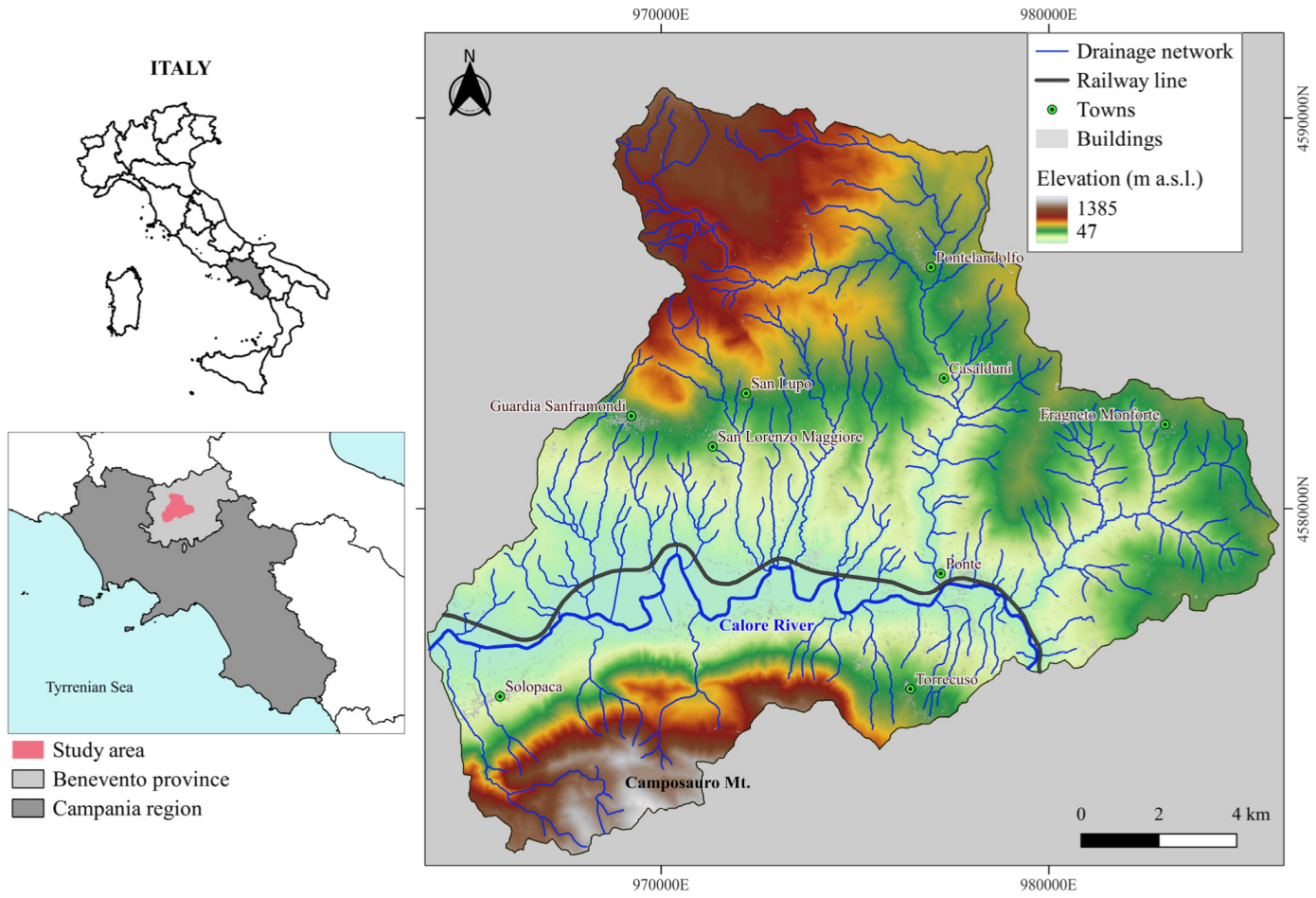
Figure 1. Study area in southern Italy with topographic elevations, drainage network, main settlements, and railway line.
Water 16 02592 g001
Figure 2. Photographic evidence of the aftermath and a map showing the position of the water-related infrastructure damage along the railway line: (a) obstruction of crossing structures (culvert/bridge), (b) clogging of drainage ditches by debris material, (c) instability/collapse of retaining walls—masonry damage, (d) failure of embankment caused by erosion, (e) overtopping of the line by water/mud from upstream. The photos are courtesy of Rete Ferroviaria Italiana (RFI).
Water 16 02592 g002
Figure 3. Flowchart of the flood susceptibility zonation framework.
Water 16 02592 g003
Figure 4. Thematic maps of the Flood-Influencing Factors in a reclassified scale from 1 (low susceptibility) to 5 (high susceptibility): (a) Elevation, (b) Slope, (c) Topographic Wetness Index, and (d) Distance to Streams.
Water 16 02592 g004
Figure 5. Thematic maps of the Flood-Influencing Factors in a reclassified scale from 1 (low susceptibility) to 5 (high susceptibility): (a) Drainage Density, (b) Geology, (c) Land Use Land Cover, and (d) cumulative two-day rainfall.
Water 16 02592 g005
Figure 6. Map illustrating the Flood Susceptibility Condition (FSC) (a) along with the upper (FSCmax) (b) and lower (FSCmin) values (c), obtained by accounting for the uncertainty in the factors’ weights.
Water 16 02592 g006
Figure 7. Map illustrating the Flood Susceptibility Assessment (FSA) for the 14th–15th October 2015 storm event (a) along with the upper (FSAmax) (b) and lower (FSAmin) values (c), obtained by accounting for the uncertainty in the factors’ weights.
Water 16 02592 g007
Figure 8. Absolute difference between the Flood Susceptibility Condition map (FSC) of Figure 6a and the Flood Susceptibility Assessment map (FSA) of Figure 7a for the study area.
Water 16 02592 g008
Figure 9. Percentage distribution of the susceptibility/influence levels (low, very low, medium, high, very high) for the eight Flood-Influencing Factors, concurring with the construction of the Flood Susceptibility Condition map (FSC) of Figure 6a and the Flood Susceptibility Assessment map (FSA) of Figure 7a, over different regions (a): (b) left and (c) right part of the floodplain, and (d) hillslope area located north of the floodplain.
Water 16 02592 g009
Figure 10. Flood susceptibility maps: (a,b) Flood Susceptibility Condition (FSC) map that excludes the triggering rainfall; (c,d) and Flood Susceptibility Assessment (FSA) map. Comparison with the distribution of flood-related damage and the official flood hazard map.
Water 16 02592 g010
Figure 11. Percentage distribution of influence/susceptibility levels (low, very low, medium, high, very high) of four Flood-Influencing Factors, (a) rainfall, (b) slope, (c) distance to streams, (d) TWI, across 22 flood-related damage sites.
Water 16 02592 g011
Figure 12. Percentage distribution of influence/susceptibility levels (low, very low, medium, high, very high) of four Flood-Influencing Factors, (a) elevation, (b) drainage density, (c) geology, (d) LULC, across 22 flood-related damage sites.
Water 16 02592 g012
Table 1. A summary of the main damage caused by the intense rainfall event of October 2015, plus a description of each of the damage types.
Type of DamageDescription of the Damage
Obstruction of crossing structures (culvert/bridge)At railway–stream intersections, sediment and debris carried by the flow accumulated, leading to the obstruction of crossing structures’ clearances and the failure of drainage facilities with corresponding potential infrastructural damage.
Instability/collapse of retaining walls—masonry damageThis type of damage affected the area where the railway line passes through the town of Ponte, with buildings flanking the line structures. Instabilities and collapses of retaining walls occurred due to issues related to increased water pressures as well as flow-related erosive phenomena.
Clogging of drainage ditchesSediment and debris materials transported by overland flow or coming from the secondary tributaries led to the obstruction of several drainage facilities.
Failure of embankment caused by erosionThe overflow of the Calore River and tributary creek breached the railway embankment and caused the washing away of ballast.
Overtopping by water/mud from upstreamMasses of mud and water traveling down the slopes due to overland flow or coming from the secondary tributaries obscured several railway segments.
Table 2. Reclassification of the selected Flood-Influencing Factors.
Factor [Unit]ClassificationSusceptibility Level
Descriptive FormScore
Elevation (E), [m a.s.l.]47–225Very high5
225–415High4
415–644Medium3
644–919Low2
919–1385Very low1
Slope (S), [°]0–6.6Very high5
6.6–12.4High4
12.4–20Medium3
20–30.7Low2
30.7–70.8Very low1
Rainfall (C2DR), [mm]305.1–415.4Very high5
252.7–305.1High4
214.4–252.7Medium3
165–214.4Low2
77.5–165Very low1
Land use land cover (LULC)Urban areasVery high5
Sparse urban areasHigh4
Agricultural landMedium3
Grassland and shrubLow2
ForestVery low1
Distance to streams (DS), [m]1st–2nd-order streams
0–25Very high5
25–50High4
50–100Medium3
100–150Low2
>150Very low1
3rd-order streams
0–50Very high5
50–100High4
100–150Medium3
150–200Low2
>200Very low1
4th-order streams
0–100Very high5
100–200High4
200–300Medium3
300–400Low2
>400Very low1
5th-order streams
0–100Very high5
100–300High4
300–500Medium3
500–700Low2
>700Very low1
Topographic wetness
index (TWI), [-]
12.47–23.62Very high5
9.00–12.47High4
7.01–9.00Medium3
5.56–7.01Low2
1.75–5.56Very low1
Geology (G)ClayVery high5
Sandstone and
arenaceous marl
High4
Marl and calcareous marlMedium3
Alluvial Low2
LimestoneVery low1
Drainage density (DD), [km/km2]2.37–3.64Very high5
1.82–2.37High4
1.31–1.82Medium3
0.75–1.31Low2
0–0.75Very low1
Table 3. Factors used in flood susceptibility mapping and their corresponding weights, as determined by the Analytical Hierarchy Process (AHP).
Flood-Influencing FactorWeights of
Factors (Using AHP)
Condition MapAssessment Map
Triggering factorRainfall (C2DR)-0.219
Conditioning
factor
Slope (S)0.2550.201
Distance to streams (DS)0.2550.201
Topographic wetness index (TWI)0.1510.116
Elevation (E)0.1510.116
Drainage density (DD)0.0920.069
Geology (G)0.0580.045
Land use land cover (LULC)0.0390.031
Table 4. Percentages representing the area of each flood susceptibility class with respect to the study area for the three Flood Susceptibility Condition (FSC) maps of Figure 6 and for the three Flood Susceptibility Assessment (FSA) maps of Figure 7.
Flood SusceptibilityFSC (%)FSCmax (%)FSCmin (%)FSA (%)FSAmax (%)FSAmin (%)
Very High13.914.214.112.512.112.4
High22.622.823.223.322.223
Medium3029.729.22929.528.8
Low202019.922.623.622.3
Very Low13.613.213.612.512.713.7
Table 5. Distribution of flood-related damage: comparison with the official fluvial flood hazard map and the flood susceptibility maps produced in this study. The symbol x means no intersection.
Intersection with
Damage #Damage TypeOfficial
Flood Inundation Map
Flood Susceptibility Condition
(FSC) Map
Flood Susceptibility Assessment
(FSA) Map
1–2Obstruction of crossing structuresx✓ Very high✓ Very high
3–5Obstruction of drainage ditchesx✓ Very high✓ Very high
6Obstruction of drainage ditchesx High✓ Very high
7–10Wall collapse/instabilityx✓ Very high✓ Very high
11–12Failure of embankment caused by erosionx✓ Very high✓ Very high
13–18Overtopping by water/mud from upstreamx✓ Very high✓ Very high
19Overtopping by water/mud from upstreamx✓ Very high High
20–22Overtopping by water/mud from upstreamx✓ Very high✓ Very high
Disclaimer/Publisher’s Note: The statements, opinions and data contained in all publications are solely those of the individual author(s) and contributor(s) and not of MDPI and/or the editor(s). MDPI and/or the editor(s) disclaim responsibility for any injury to people or property resulting from any ideas, methods, instructions or products referred to in the content.