Article

Monitoring of Total Phosphorus in Urban Water Bodies Using Silicon Crystal-Based FTIR-ATR Coupled with Different Machine Learning Approaches

1
The State Key Laboratory of Soil and Sustainable Agriculture, Institute of Soil Science, Chinese Academy of Sciences, Nanjing 210008, China
2
College of Modern Advance Agricultural Science, University of Chinese Academy of Sciences, Beijing 100049, China
*
Author to whom correspondence should be addressed.
Water 2024, 16(17), 2479; https://doi.org/10.3390/w16172479
Submission received: 9 July 2024 / Revised: 13 August 2024 / Accepted: 26 August 2024 / Published: 31 August 2024
(This article belongs to the Section Urban Water Management)

Abstract

:
Eutrophication occurs frequently in urban water bodies, and rapid measurement of phosphorus (P) is needed for water quality control, since P has been one of the limiting factors. In this study, approximately 400 water samples were collected from typical urban water bodies in Nanjing city, and Fourier transform infrared attenuated total reflectance spectroscopy (FTIR-ATR) was applied for rapid P determination. Both silicon ATR (Si-ATR) and ZnSe-ATR were employed in the recording of FTIR-ATR spectra, and different algorithms, including partial least squares regression (PLSR), support vector machines for regression (SVRs), extreme learning machines (ELMs), and self-adaptive partial least squares model (SA–PLS), were applied in the analysis of spectra data. The results showed that the water quality varied significantly for different water bodies in different seasons, and both Si-ATR and ZnSe-ATR could achieve good P prediction. The PLSR and SVR models showed poor P prediction effects while the ELM model was excellent, and the SA-PLS model was the best one. For the SA-PLS model, the prediction accuracy of Si-ATR (Rv2 = 0.973, RMSEV = 0.015 mg L−1, RPDV = 6.05) was slightly better than that of ZnSe-ATR (Rv2 = 0.942, RMSEV = 0.011 mg L−1, RPDV = 4.13). Therefore, the FTIR-ATR technology coupled with the SA-PLS model achieved rapid P determination in urban water, providing an effective option for water quality monitoring.

1. Introduction

Phosphorus (P) is one of the essential nutrients for plant growth [1], and excessive P input has resulted in eutrophication of water bodies and the further formation of harmful algal blooms [2,3], which cause environmental damage by producing toxins, consuming dissolved oxygen and threatening human and wildlife health [4,5]. Urban water is an important part of the urban environment, and over the past few decades, rapid urbanization has brought water-related problems to cities around the world, including water shortages and declining water quality. This degraded water quality directly affects a city’s drinking water and recreational water [6]. Qinhuai River is the largest river in Nanjing. As an important agricultural irrigation water source and water transport channel of Nanjing, it plays an important role in the development of Nanjing city and its surrounding areas. In recent years, with a change in agricultural land use types along the river, the rapid development of industry and the dramatic increase in residential population, farmland runoff, industrial wastewater and domestic sewage accepted by the Qinhuai River have also doubled, resulting in different degrees of eutrophication of the river [7]. The structure and function of this kind of water ecosystem are relatively simple, showing the characteristics of a small water area, weak water circulation, weak self-regulation ability and great influence from human activities [7,8]. In such aquatic ecosystems, timely acquisition of the water’s phosphorus content is critical for controlling eutrophication [9].
The conventional methods for P determination in water include ammonium molybdate spectrophotometry, ion chromatography and the stannous oxide reduction molybdenum blue method, but these methods are time- and cost-consuming. As a fast and non-destructive analysis method, Fourier transform infrared attenuated total reflectance spectroscopy (FTIR-ATR) has the advantages of a simple analysis process, low cost, high efficiency and no chemical reagents [10]. Previous studies on FTIR-ATR of phosphorus have mostly focused on qualitative analysis, and the quantitative analysis of phosphorus remained unclear [11,12] due to the weak target signal and the strong interference [13,14]. Meawhile, we successfully achieved the qualitative analysis of TP in a solution using the water subtraction algorithm [15]. The most widely used crystal of ATR accessories is ZnSe, which takes on a high refractive index, but the crystal is extremely fragile, easy to wear and expensive, while a Si crystal can be used in acid and alkali situations and is much cheaper than the conventional ZnSe crystal [10,16]. Therefore, it is necessary to explore the capability of Si-ATR in P monitoring when combining chemometrical methods.
Machine learning algorithms are powerful in their ability to reveal the relationship between spectra and substance concentrations, and the performance of different algorithms needs to be optimized [17]. Partial least squares regression (PLSR) is an effective algorithm for solving the problem of composition detection in water [18]. Considering that the composition of a real water environment is relatively complex, spectral data are subject to being disturbed, and when dealing with nonlinear correlated problems, the performance declined significantly. Therefore, it is essential to establish an applicable, robust and acceptable prediction model, and support vector machines for regression (SVRs) and extreme learning machines (ELM) were recommended for practical applications of complex, highly nonlinear objects [19]. The SVR and ELM models can handle both linear and nonlinear relationships [20], but the problem of overfitting is easily encountered in the case of a small number of training samples. Aside from the algorithm model, the size of the calibration set affected the prediction performance [21]. Accuracy increases with the number of objects in the calibration set and tends to stabilize when the number of samples is representative enough [22]. The self-adaptive partial least squares (SA-PLS) model can accurately predict organic matter in complex soil systems [23]. It has showed obvious advantages in the selection of calibration samples and can obtain better prediction results [22], which can be employed in water samples.
In this study, FTIR-ATR technology coupled with multiple machine learning methods (PLSR, SVR, ELM and SA-PLS) is explored to develop a robust method for rapid quantitative quantification of TP in urban water bodies, and the effects of ATR crystals, data pretreatment methods and modeling algorithms are considered and optimized, which will provide an option for the monitoring of water quality.

2. Materials and Methods

2.1. Water Sample Collection and Determination of Physical and Chemical Properties

A total of 100 typical sampling points were set up for collecting water samples in Nanjing, Jiangsu Province, China (Figure 1). The sampling points numbered 1–24 and 75–88 were typical lake water samples, and 25–74 and 89–100 were representative river water samples. The samples were collected in different months and seasons, namely April (spring), August (summer), November (autumn), and February (winter). Water samples were collected at a depth of 0.5 m and stored in a glass bottle without any pretreatment. The temperature and pH level were measured in situ using a portable water quality parameter meter. Each water sample was digested through the persulfate method, and the P content was determined through the molybdate blue spectrophotometric method. ICP-AES (ICAP 6000, Thermo Fisher Scientific, Waltham, MA, USA) was used to measure the sulfate content.

2.2. Spectra Measurements

The samples were scanned using a Si attenuated total reflection (Si-ATR) single-reflection sampling module cell and a ZnSe attenuated total reflection (ZnSe-ATR) multiple-reflection sampling module cell mounted on a Nicolet 6700 spectrophotometer instrument (Thermo Fisher Scientific). The scans were conducted in the wavenumber region of 4000–800 cm−1 with a resolution of 4 cm−1 and mirror velocity of 0.32 cm s−1. Thirty-two successive scans were recorded and averaged. The spectra of deionized water were recorded as reference blank spectra for subsequent subtraction. ATR correction was carried out in the acquisition process for avoiding spectral deformation. Since the absorbance values of the phosphate peaks were extremely low, the infrared-enhanced light source was selected. Each sample was measured three times to take the average for data analysis. The ATR crystal was cleaned with ethanol and denoised water before every new sample measurement. The background spectra and each sample spectrum were measured within less than 2 min.

2.3. Preprocessing of Spectra

Firstly, a morphological weighted penalized least squares algorithm was used for baseline corrections of all raw spectra [24]. Second, a water subtraction algorithm [25] was applied to the obtained spectra. Third, the spectra were smoothed with a Savitzky–Golay filter [26]. Then, other preprocessing techniques or their combinations were applied, including the first derivative (FD) and second derivative (SD) of absorbance, to reduce baseline variation and enhance the spectral features [27] and mean centering (MC) [28]. Then, the processed spectra were used to establish the predicted models. The data of the water samples were randomly divided into two sets, namely a calibration set and a validation set, containing 70% and 30% of the samples, respectively. Data processing was conducted using MATLAB R2018a (Mathworks, Natick, MA, USA).

2.4. Prediction Models

PLSR was proposed by Wold et al. [29] and has become a widely used method for multivariate calibration in analytical chemistry [30] which demonstrates the features of avoiding multicollinearity and reducing noise and computation time [31]. The PLSR method has been applied for the quantitative analysis of phosphate, adopting leave-one-out cross-validation [32]. Compared with conventional PLSR, the SA-PLS model selected suitable samples according to spectra similarity as a calibration set [21]. Therefore, the SA-PLS model was developed in two steps: (1) the Euclidean distance was involved to identify the samples, and then (2) the sample numbers for modeling were optimized. The Euclidean distance was defined as shown in Equation (1):
E D i j = x = 1 p ( A x i A x j ) 2
where EDij is the Euclidean distance of the ith unknown sample and the jth calibration sample; i, j = 1, 2, …, n; ji. x is the number of variables in the spectrum and x = 1, 2, 3, …, p. In this paper, p, which is the whole number of variables in the preprocessed spectra used for modeling, is 182. A is the absorbance of the corresponding spectra. Then, according to their EDij values, the samples similar to the target sample were reordered in ascending order. The following step was to optimize the calibration numbers and build models. The size of the calibration sets was set in the range of 10–280 with intervals of 5 to ensure the optimal calibration set. Five parameters—RPD, SD, R2, RMSEv and RMSEv/RMSECV—were used to optimize the number of calibration samples. After optimization of the calibration numbers, the PLS model was built to predict the TP content of the unknown sample.
The SVM is a machine learning method developed on the basis of statistical learning. SVMs can execute classification and regression. Support vector machines for regression (SVRs) apply a kernel function including the linear function, polynomial function, Gaussian radial basis function (RBF) and sigmoid function [33] to map the input variables into a high-dimensional feature space [30]. SVM-based techniques have the ability to model nonlinear relationships. Gaussian RBF was applied, and the capacity parameter (C) and kernel parameter of the RBF (γ) of the SVR were optimized through the grid searching method. For the SVR calculations, the MATLAB toolbox LIBSVM (version 3.24), developed and described by Chang and Lin [33], was used. The ELM is an emerging optimization technique proposed for training single hidden layer feedforward neural networks (SLFNs). Although the hidden nodes are randomly generated, ELMs still maintain the universal approximation capability of SLFNs [34]. The connections (or weights) between the hidden and output layer are the only free parameters which need to be optimized. The ELM algorithm was executed with MATLAB’s Extreme Learning Machine toolbox.

2.5. Model Evaluation

The coefficients of determination (R2), root mean square error (RMSE), and residual prediction deviation (RPD) of the calibration and validation sets were determined as the evaluation index of all models for the purpose of evaluating the accuracy and generalization ability of the models (Equations (1)–(3)). RC2 and RV2 are the determination coefficients of the calibration set (C) and validation set (V), respectively; RMSECV, RMSEC, and RMSEV are the root mean square errors (mg L−1) of the cross-validation set (CV), calibration set, and validation set, respectively; and RPDC and RPDV are the residual prediction deviations of the calibration set and validation set, respectively:
R 2 = 1 i = 1 n y i y ^ i 2 i = 1 n y i y ¯ i 2
R M S E = i = 1 n y i y ^ i 2 n
R P D = S D R M S E
where y i and y ^ i are the measured and predicted values of the ith sample, respectively, y i is the average of measured values, and n is the number of samples. SD is the standard deviation of the measured values. An RPD value less than 1.8 was considered unsuitable for quantitative measurement, and 2 < RPD < 2.5 indicated good model prediction performance, while RPD > 3 indicated excellent prediction performance. This classification system was adopted in this study [25,35], where a larger R2 value demonstrated a better model fitting effect, and a smaller RMSE indicated better model prediction accuracy. In this study, the model with the highest R2 and RPD values, along with the lowest RMSE, was involved in optimization.

3. Results and Discussion

3.1. Properties and Characteristics of Natural Water Samples

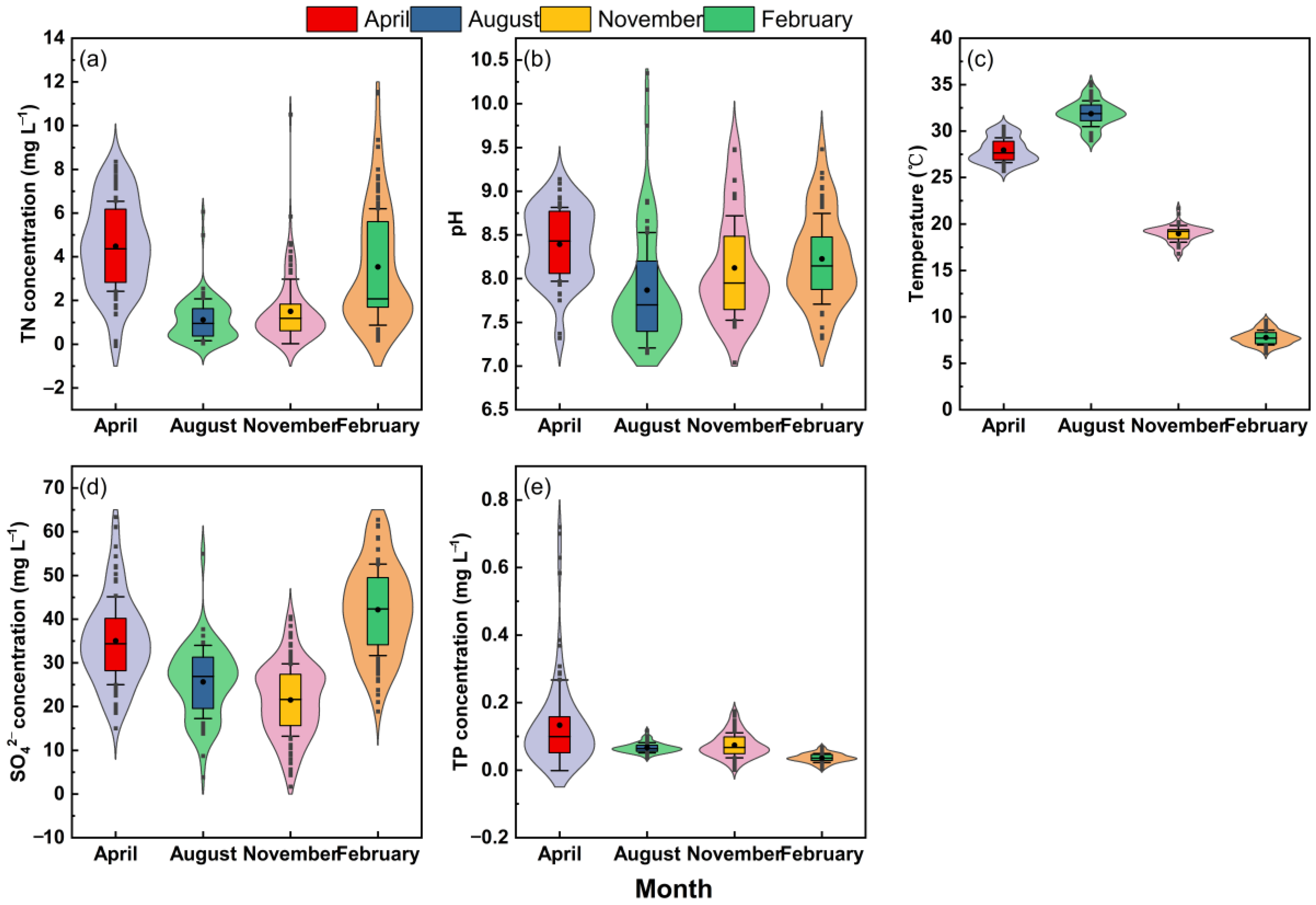
Figure 2 shows the results of the statistical analysis of the water quality indexes of water samples in different seasons. The average TP content was 0.133 mg L−1 in spring, 0.066 mg L−1 in summer, 0.074 mg L−1 in autumn, and 0.036 mg L−1 in winter. The variation range of the TP index in the four seasons was 0.001–0.72 mg L−1, and the coefficient of variation was 100.9%, 22.9%, 50.2%, and 38%, respectively, indicating that the distribution of the total phosphorus content in spring and autumn was significantly different. Only 4 of the 400 samples had a TP concentration higher than the standard limit value of 0.4 mg L−1, which was stipulated in the Environmental Quality Standards for Surface Water (GB 3838-2002). The variation in TN content in the four seasons ranged from 0.030 to 11.555 mg L−1, and the coefficient of variation ranged from 45.9% to 98.5%, indicating that there were great differences in the distribution of total nitrogen. The water temperature varied greatly with the seasons. The temperature of the water affected many physical and chemical properties of the water. The mean and minimum pH values of the water were greater than seven in spring, summer, autumn, and winter. The mean value of the sulfate content in the four seasons was less than 43 mg L−1, and none of the samples exceeded the standard limit of 250 mg L−1.
As shown in Figure 2, the average TP concentration in April was significantly higher than that in other seasons, reaching 0.133 mg L−1. This may be related to the frequent agricultural activities. A large amount of phosphate fertilizer was flushed into water through high rainfall [36], resulting in a decline in water quality [37]. The TP concentration in August was at a lower level of 0.066 mg L−1. The reason for this trend could be higher water temperatures in August resulting in an abundance of plankton in the water. This increased the uptake and utilization of P in the water, thus depleting the reactive phosphate [38]. August is the rainy season, which has a particularly significant dilution effect on the TP concentration in water bodies. The TP concentration in February was at a low level of 0.036 mg L−1. During this period, the temperature and precipitation were low, and the biological growth and reproduction cycle as well as various physical, chemical, and biological activities were at a low level.
The pollution sources of phosphorus in water mainly include exogenous pollution sources and endogenous pollution sources. Exogenous pollution sources mainly include agricultural drainage, domestic sewage, and industrial wastewater, as well as surface runoff, soil erosion, precipitation, aquaculture, rock weathering release, and atmospheric input. The economic development level, industrial production structure, and land use and population are the main factors contributing to the net phosphorus input [39]. Our sampling sites were generally located in areas with frequent human activities, where the population was densely distributed and there were many industrial and mining enterprises and buildings. Human activities directly discharged untreated domestic sewage and industrial wastewater into rivers, which had a great impact on the water quality [40]. Urban domestic sewage contains a large amount of phosphorus from synthetic detergents. Industrially, production activities such as industries, mines, and enterprises discharged a large amount of phosphorus-containing wastewater [4]. In addition, the endogenous pollution of phosphorus in water mainly comes from the sediment of rivers and lakes. Sediment is a reservoir of nutrients. When exogenous pollutants are effectively controlled, the release of nutrients from sediments is also an important cause of water eutrophication [41]. Sediments can adsorb or release phosphorus [42,43], which also leads to dynamic changes in TP in the water body.

3.2. FTIR-ATR Spectra of Natural Water Samples

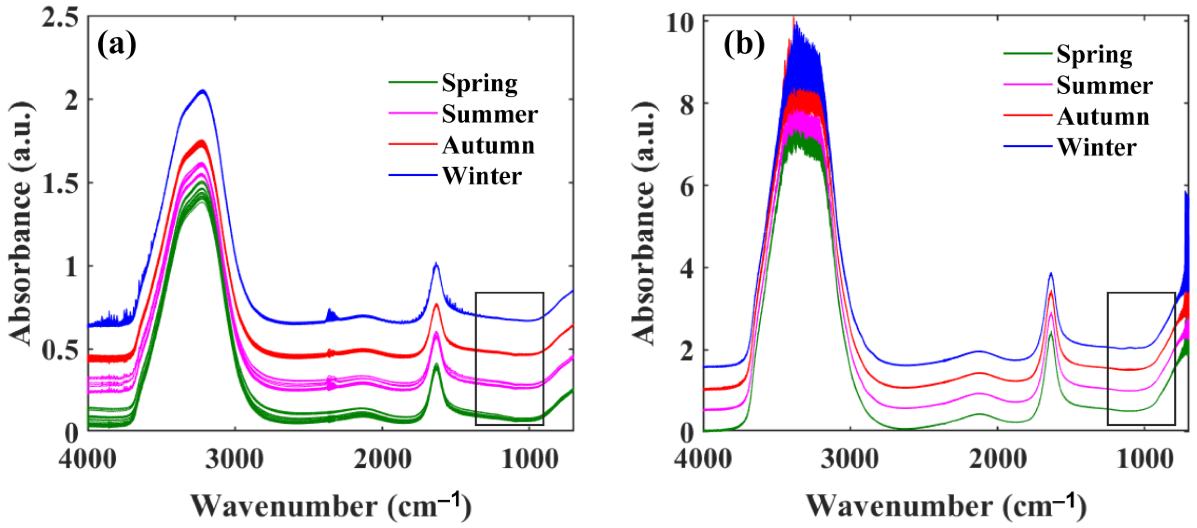
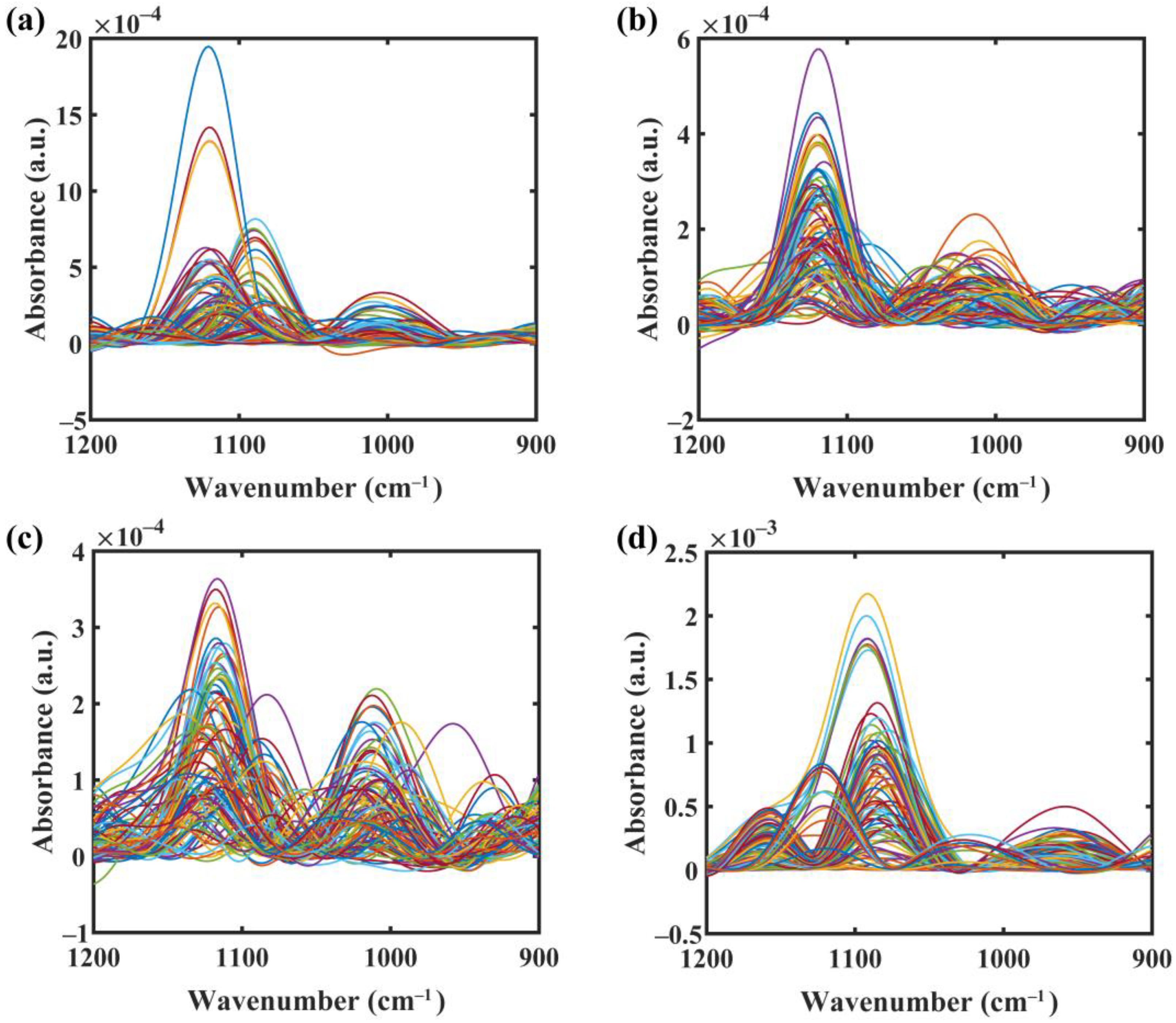
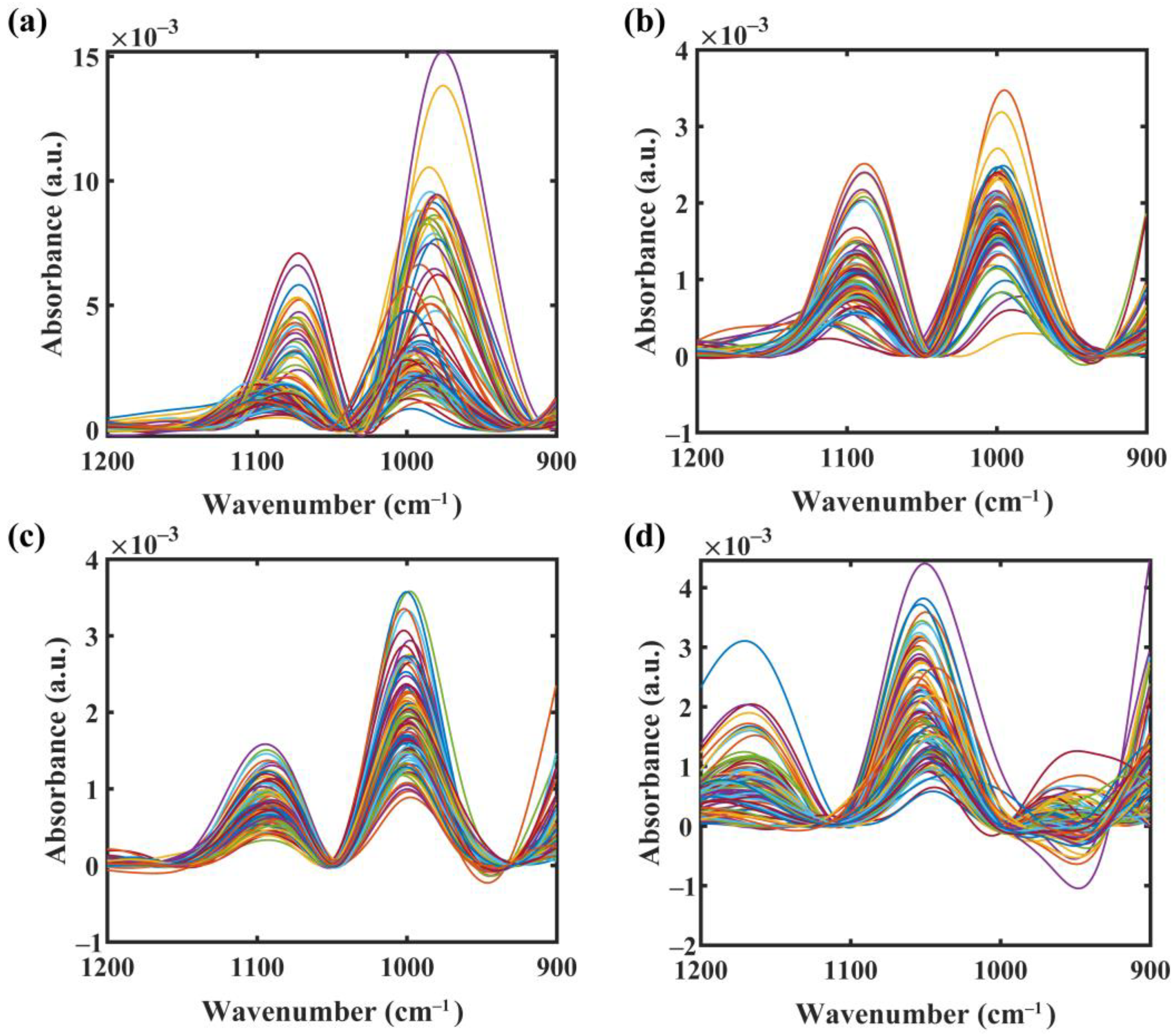
Figure 3 shows the FTIR-ATR spectra of natural water samples in different seasons from Nanjing. The spectra of water samples obtained with two crystal materials in different seasons were basically the same shape, and there were two obvious absorption peaks in the bands of 3800–2800 cm−1 and 1800–1500 cm−1, which are characteristic of the absorption of water. The characteristic bands of phosphate were located in the 1200–900 cm−1 band. Because the absorption bands of phosphate are weak and subject to water molecular interference, it is difficult to observe with the naked eye. Therefore, it was necessary to further conduct signal processing on the original spectra to obtain effective spectral information from complex signals. After water deduction, baseline correction, and smoothing, the absorption band of the target signal became clearly visible. In order to reduce noise and retain target information, the spectral range of 1200–900 cm−1 was specifically considered. After pretreatment, the FTIR-ATR spectra of the water samples showed several characteristic absorption peaks related to phosphorus (Figure 4 and Figure 5).
The FTIR-ATR spectra of the water samples obtained from the two crystal materials were quite different. The absorbance of the absorption peak of the ZnSe-ATR spectrum was 1–2 orders of magnitude larger than that of the Si-ATR spectrum, which resulted from the differences in the length and thickness of the ATR crystal materials. ZnSe-ATR was multiple-reflection ATR, while Si-ATR was single-reflection ATR. The peak number, peak intensity, and peak position of the characteristic peaks of the water samples obtained from different crystals in different seasons were obviously different. The centers of the characteristic peaks were located at 1161 cm−1, 1076 cm−1, 990 cm−1, and 940 cm−1. The intensity of the peak was related to the TP concentration. Therefore, these characteristic peaks can be used to predict the TP content in water quickly.

3.3. PCA Analysis

The PCA results of the FTIR-ATR spectra of the water samples in this study area are shown in Figure 6. For the Si-ATR spectra, the variation explanations of the first three principal components reached 69.99%, 20.2%, and 4.5%, and the total variation explanations of the first three principal components reached 94.69%. For the ZnSe-ATR spectra, the variance interpretation of the first three principal components reached 69.52%, 17.41%, and 5.4%, and the total variance interpretation of the first three principal components reached 92.33%, which indicates that the first three principal components of the spectra obtained from the two ATR attachments could cover the vast majority of the spectra information. According to the scatter plots of the first three principal component scores (Figure 6c,d), the dispersion of Si-ATR spectra of the four seasons was divided into two categories. The dispersion points of the winter sample data were relatively scattered and far away from the dispersion points of spring, summer, and autumn, and the dispersion points of spring, summer, and autumn were clustered into one category. The scattered points of the principal component scores of ZnSe-ATR fell into three categories. The scattered points of summer and autumn fell into one category, and the scattered points of spring and winter fell into one category, which indicate that the seasonal variation of the FTIR-ATR spectra of the water samples in the study area was large.

3.4. Prediction of TP in Water Based on Si-ATR and ZnSe-ATR

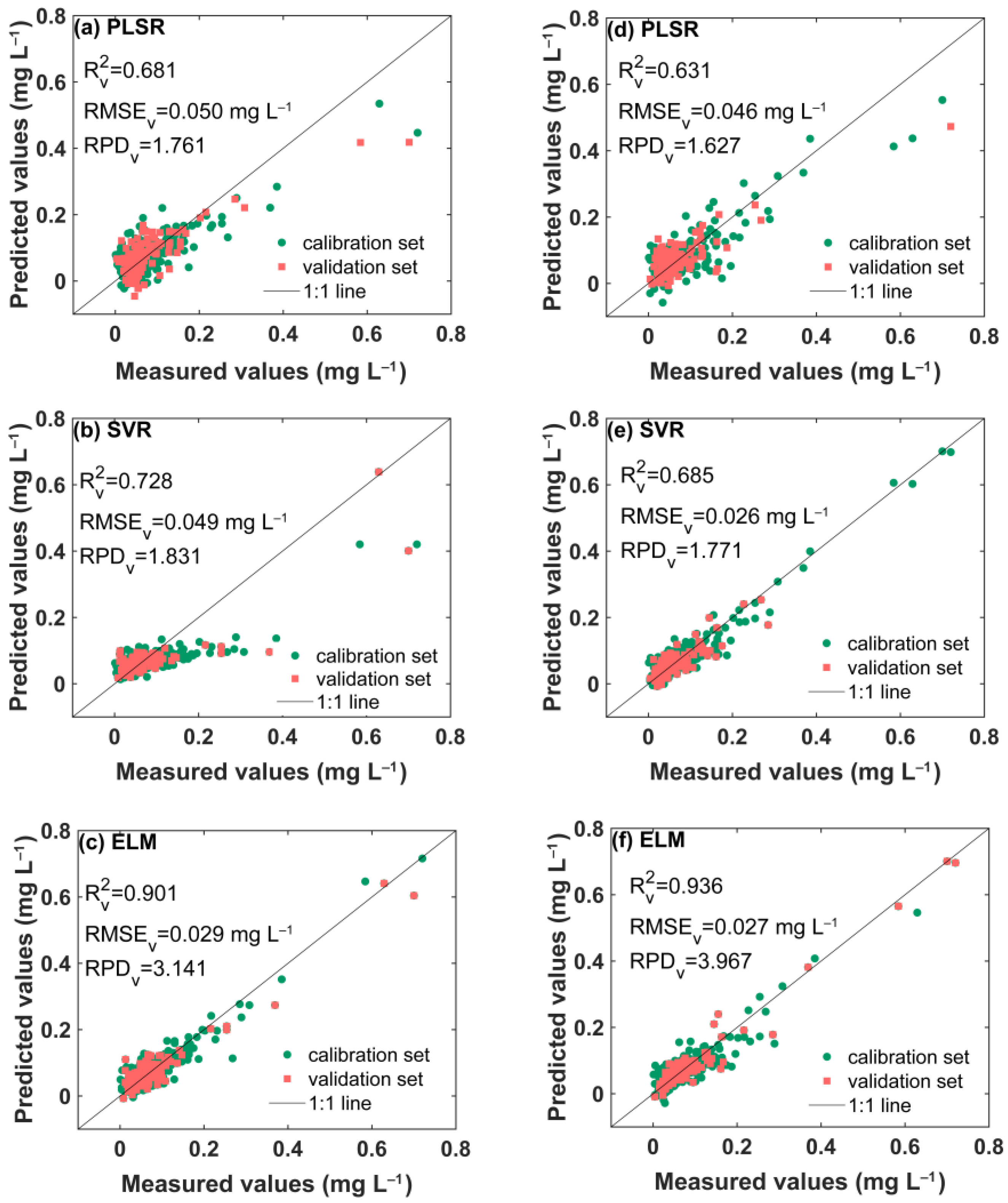
The raw spectral data obtained by the Si-ATR and ZnSe-ATR accessories were preprocessed, and then a wavenumber in the range of 1200–900 cm−1 was selected for modeling. Three different machine learning algorithms, PLSR, SVR, and ELM, were used to establish the quantitative analysis models of TP in water. A total of 400 samples collected from Nanjing city in four seasons were randomly divided into two groups according to a ratio of 7:3, in which 280 samples were used as a calibration set and 120 samples were used as a validation set. The modeling results are shown in Figure 7.
The effects of the base preprocessing, mean centering (MC), first derivative (FD), and second derivative (SD) preprocessing on PLSR model performance were focused upon, and the results are shown in Table 1. For the Si-ATR spectral data, the PLSR modeling results of the base, MC, FD, and SD preprocessed data were significantly improved compared with the model results for the original data. Among them, the results of the base treatment were optimal compared with those of the MC, FD, and SD treatments (Rv2 = 0.681, RMSEV = 0.050 mg L−1, RPDV = 1.761) but did not meet the requirements of quantitative analysis (RPD value less than 1.8). Therefore, the data preprocessed with the base treatment were used in the subsequent modeling, and no other preprocessing was performed.
For the ZnSe-ATR spectral data, similarly, the PLSR modeling results of the base, MC, FD, and SD preprocessed data were significantly improved compared with the raw spectra data. Among them, the PLSR modeling result of the base + FD preprocessed spectral data was the best (Rv2 = 0.683, RMSEV = 0.053 mg L−1, RPDV = 1.744), and thus the subsequent modeling data all used the base + FD processed data.
These results indicate that proper spectral preprocessing was able to improve the prediction accuracy of the model compared with the raw data. The FTIR spectra technique has some shortcomings, such as a low signal-to-noise ratio, large fluctuation, and serious overlapping of peaks. Consequently, it is necessary to use all or part of the spectra of samples in the qualitative and quantitative analysis, as more involved wavebands resulted in more effective target information, while the interfering wave increase might lead to a decline in prediction accuracy. Therefore, the selection of pretreatment methods and spectral variables was the foundation for establishing a model with good robustness and prediction ability.
Many mathematical algorithms were applied to preprocess the raw spectra for improving estimation accuracy. The infrared spectrum of complex samples was the superposition of the spectral bands of different components, and the mutual interferences between the components were serious, while the derivative could improve the resolution and sensitivity of the spectrum and would improve the multicollinearity to a considerable extent. Consequently, the performance of the prediction model significantly improves. However, the signal-to-noise ratio of the spectrum becomes lower with the increase in the derivative order, and the prediction error increases [28]. Thus, in practical applications, first-order and second-order differential spectra are generally used, while third-order or more differential spectra are rarely applied. Application of the first and second derivatives of absorbance in phosphate concentration estimation depends on the quality of the raw spectral data. Some studies employed the first derivative [44,45], while others preferred the second derivative [46].
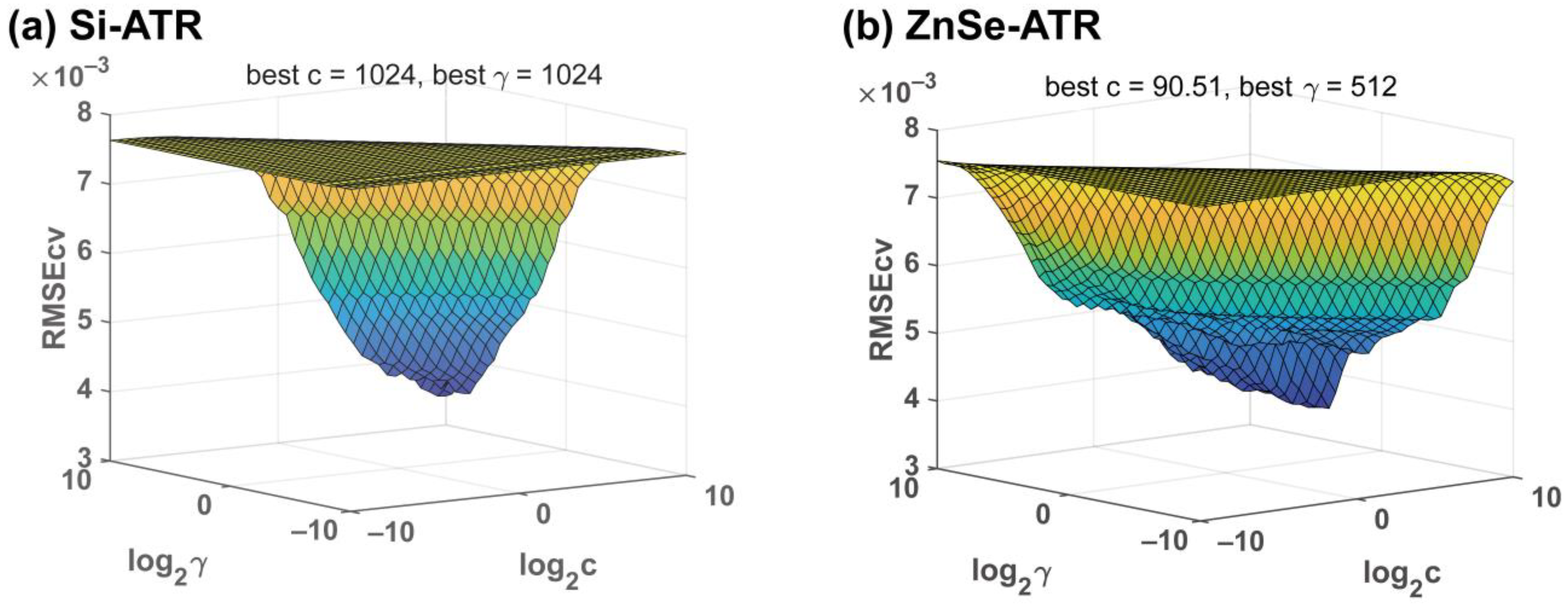
Figure 7 shows the differences between the two crystals in the quantitative analysis of PLSR. The Rv2, RMSEV, and RPDV values of the Si-PLSR model were slightly better than those of the ZnSe-PLSR model. For the Si-ATR and ZnSe-ATR spectra, the PLSR modeling results could not be used for quantitative analysis of the TP content in water quality (RPD < 1.8). Accordingly, other nonlinear machine learning models were used to predict the TP content in water. After optimal preprocessing of the spectra, the SVR and ELM models were used to predict the TP content. As for SVR, Gaussian RBF was applied, and the capacity parameter of SVR (c) and the kernel parameter of RBF (γ) were optimized by the grid searching method. The optimized parameters were applied to establish the Si-SVR (c = 1024, γ = 1024) and ZnSe-SVR (c = 90.51, γ = 512) models (Figure 8). As for the ELM model, the number of cryptic nerve nodes was 120. The scatter plots of the measured values versus the predicted values of the TP content are shown in Figure 7.
For the Si-ATR, the RPDV value of PLSR was less than 1.8, indicating that the model was not reliable. However, the RPDV values of the SVR and ELM models were all greater than 1.8, indicating that these models could be used for quantitative prediction of the TP content in water. Among them, the ELM model had the best prediction effect (Rv2 = 0.901, RMSEV = 0.029 mg L−1, RPDV = 3.141), followed by the SVR model (Rv2 = 0.728, RMSEV = 0.049 mg L−1, RPDV = 1.831). In comparison with the Si-ATR models, for ZnSe-ATR, the RPDV value of the PLSR was 1.627, indicating that the model was not suitable for quantitative prediction of the TP content. In addition, the RPDV values of the SVR model were less than 1.8. In contrast, the ELM model had the best prediction effect (Rv2 = 0.936, RMSEV = 0.027 mg L−1, RPDV = 3.967), indicating that the models could be used for quantitative prediction of the TP content in water. For both the Si- and ZnSe-ATR data, it was clear that the predictive performance of the ELM models was superior to the other models, which is consistent with the scatterplot results shown in Figure 7, and the scatters of the ELM models were closer to the 1:1 line than the other models.
Although the ELM model achieved good prediction results, there were some problems in the ELM model itself. The selection of the number of hidden neurons played a crucial role in the generalization performance of the network. However, the selection of cryptic neurons did not form a unified and reasonable method. When the size of the training sample set was small, it was prone to overfitting.

3.5. Effect of Season Variation on TP Prediction

Our previous study [15] showed that the PLSR prediction effect of P in a standard solution was excellent, but the prediction effect in natural water samples was greatly degraded (Figure 7), which might have been due to the large variation range of the TP content in actual water samples, the increase in interfering substances in actual water samples, such as the presence of sulfate, which affected the characteristic peak of P, and the change in pH of the water body, which also caused a change in spectra. The PCA clustering results of the water sample spectra in different seasons were different (Figure 6), which indicates that the water spectra were related to seasonal changes. We therefore investigated the influence of the season on PLSR prediction, and the results are shown in Table 2.
The samples of four seasons in Nanjing were randomly divided into calibration sets and validation sets according to a ratio of 3:1, and the PLSR method was used to establish quantitative prediction models for the TP content in natural water samples in different seasons. The spectra associated with the TP content in the 1200–900 cm−1 range collected by the Si-ATR and ZnSe-ATR accessories after pretreatment were utilized for the models. The cross-validation method was used to obtain the optimal number of principal components for the PLSR model in different seasons. For the Si-ATR data, the optimal number of principal components for the spring, autumn, summer, and winter models was 6, 8, 9, and 10, respectively. Based on this, the optimal PLSR model for each season was established. The RC2 values between the measured and predicted values in the four seasonal calibration sets were 0.897, 0.707, 0.774, and 0.791, respectively. The RV2 of the validation set was 0.863, 0.745, 0.728, and 0.809, respectively. The RMSEV values were 0.049, 0.008, 0.022, and 0.006 mg L−1, respectively. The RPDV values were 2.401, 1.904, 1.836, and 2.19, respectively, which were higher than the minimum standard of 1.8 required for quantitative detection. The prediction bias was close to zero, except for 0.007 mg L−1 in spring. The predictive performance of all four models mentioned above achieved excellent results and could be used for the determination of the total phosphorus content in water. For the ZnSe-ATR spectra, the modeling effect was similar to that of the Si-ATR spectra. The optimal number of principal components of the PLSR model for the four seasons was 6, 13, 9, and 9, respectively. The RV2 values between the measured and predicted values in the validation sets of the four seasons were 0.763, 0.743, 0.707, and 0.744, respectively. The RMSEV values were 0.078, 0.008, 0.017, and 0.007 mg L−1, respectively. The RPDV values were 2.053, 1.918, 1.838, and 1.902, respectively. The prediction bias of the four PLSR models was close to zero, and an accurate prediction effect was obtained.
In terms of modeling effectiveness, the modeling effect of Si-ATR was slightly better than that of ZnSe-ATR. The best modeling results were obtained for the spring water samples followed by the winter water samples, and the modeling results for the summer and autumn water samples were relatively similar. The reasons for this modeling result may include the absorbance value of the characteristic peak of the spectra of the spring and winter water samples varying in a large range (Figure 4 and Figure 5), the characteristic peaks of the spectra being obvious, the dispersion point distribution of the principal component of the spectra being relatively scattered (Figure 6), and the data having large variance and variability (Figure 2) such that the performance of the model was relatively good. However, the absorbance values of the characteristic peaks of the spectra in summer and autumn varied in a small range, the spectra were messy, the scattering points of the principal components of the data were relatively concentrated, and the variance of the data was small, not having good sample representation and variability. Thus, the performance of the model was poor.

3.6. Application of SA-PLS Models

The predictive performance of the PLSR model using the entire dataset of 400 samples was found to be inferior to that of the seasonal samples. Furthermore, the modeling outcomes varied significantly in the four seasons, primarily due to disparities in the selection of samples for modeling. It is evident that the choice of modeling samples had a substantial influence on the accuracy of the predictions. Selecting appropriate samples for modeling can lead to obtaining excellent prediction results. Therefore, we implemented a modeling strategy called SA-PLS, which focuses on selecting similar samples to the model.
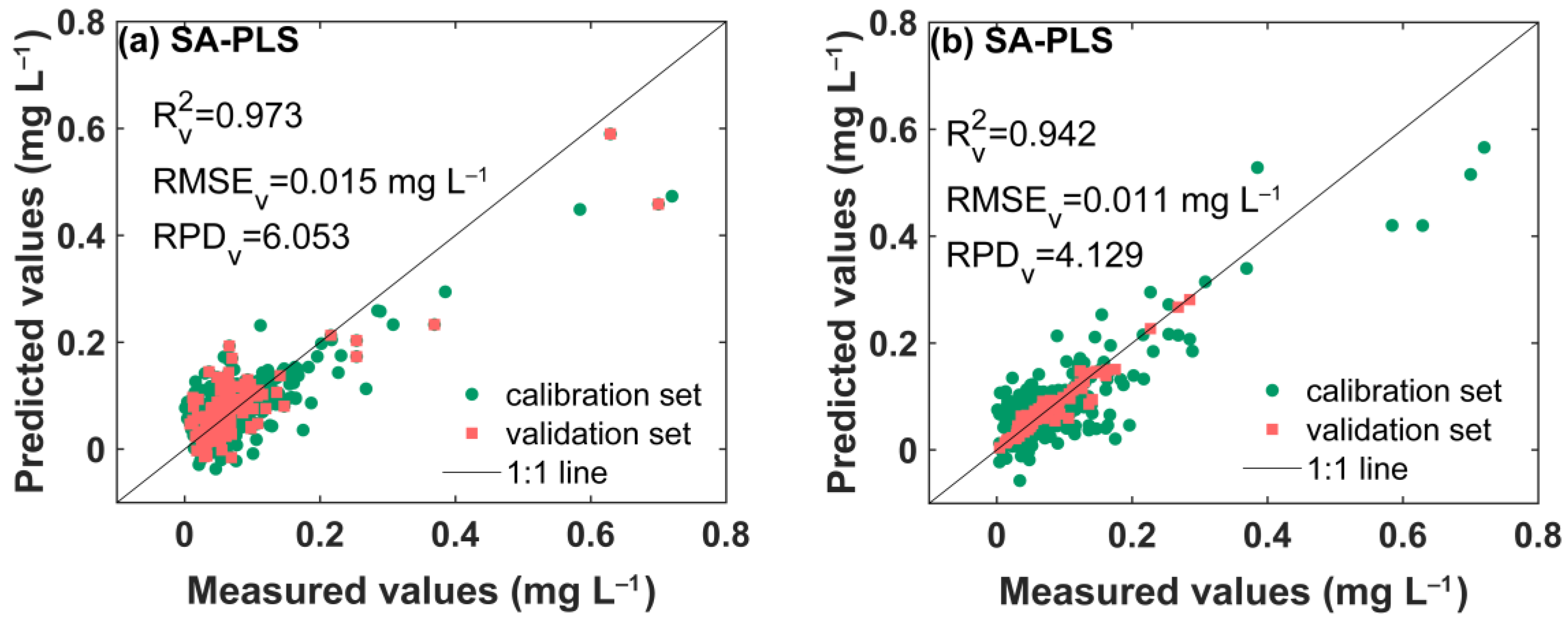
The 400 samples were randomly divided into a calibration set and validation set at a ratio of 7:3. The SA-PLS model results are shown in Figure 9. The RPDV values of the SA-PLS models were all greater than 1.8, implying excellent prediction accuracy (Figure 9a,b). For the TP prediction in the water using Si-ATR, the SA-PLS models (Rv2 = 0.973, RMSEV = 0.015 mg L−1, RPDV = 6.053) provided better prediction accuracy than when using ZnSe ATR (Rv2 = 0.942, RMSEV = 0.011 mg L−1, RPDV = 4.129). The results showed that the SA-PLS model significantly improved the TP prediction accuracy compared with the conventional PLSR model and the nonlinear SVR and ELM models.
The optimal model for each sample was obtained according the strategy of SA-PLS modeling, and each optimal model was decided by each unknown sample and therefore built based on a different calibration set. For each sample to be tested, five parameters (RPD, SD, RMSEV, R2, and RMSEV or RMSECV) were used as criteria to determine the optimal size of the 120 calibration sets. Figure 10 shows the statistics of the best calibration set size for the SA-PLS model predicting the TP content for each sample to be tested. For the Si-ATR spectra, the optimal sample size of the calibration set was 25 (73.33%), which was dominant, followed by 50 (20%), and then the optimal sample sizes were 75 and 100 (2.5%, 2.5%). For the SA-PLS model, the optimal sample size of the calibration set was more than 100, accounting for only 1.66% of the total sample number of the validation set. For the ZnSe-ATR spectra, 60% of the validation samples had an optimal calibration set size of 25, 11.67% of the samples to be tested had an optimal calibration set size of 50, and only 3.34% of the validation samples had an optimal calibration set size of more than 100.
The prediction accuracy declined compared with the results of the ideal solution due to the complexity of the natural water samples. PLSR has been developed to remain a standard tool in chemometrics [47], and it has been widely used as a regression technique for spectroscopic data analysis. However, compared with the other three models, PLSR was not good at predicting the phosphate concentration in this study. Many previous studies have shown that PLSR performs well when dealing with linear correlation problems, whereas the performance obviously degrades when dealing with nonlinear correlation problems. Hence, it might be that there were nonlinear interferences in the natural water samples. On the one hand, the absorption peaks’ positions and the strengths of different protonation phosphates were significantly different, indicating that the pH level had an important effect on the phosphate spectra. On the other hand, the absorption bands of other coexisting substances in the actual water samples also interfered with the phosphate groups. The SVR, BPNN, and ELM models were able to handle both the linear and nonlinear relationships. Support vector machines, based on the structural risk minimization principle, are usually more flexible and have better generalization performance compared with conventional statistical or machine learning algorithms [48]. Different from SVMs, which usually request two parameters (C, γ) to be specified by users, a single-parameter setting makes ELMs easy and efficient to use. Compared with SVMs, ELMs showed similar or better generalization performance for regression cases [49]. Considering the robustness, the SVM and ELM models are recommended for practical applications involving complicated, highly nonlinear objects [19].

4. Conclusions

The FTIR-ATR technique, combined with different machine learning models (PLSR, SVR, ELM, and SA-PLS), was successfully applied in the qualification of TP concentrations in the natural water bodies in Nanjing, and there were significant differences in the water quality indexes in different seasons. Both Si-ATR and ZnSe-ATR obtained accurate predictions. The PLSR model had poor TP prediction, while the ELM model and SA-PLS model had excellent prediction effects, and the SA-PLS model had the best prediction. In practical applications, the ELM model might have overfitting problems, and thus it is recommended to use the SA-PLS model. FTIR-ATR technology combined with the SA-PLS model was successfully applied to the quantitative analysis of the total phosphorus concentration in urban water samples, with Rv2 = 0.973, RMSEV = 0.015 mg L−1, and RPDV = 6.05, meaning it could be an alternative option for the determination of the TP content. In future studies, this method should be validated with more datasets to obtain more reliable and robust models for practical applications.

Author Contributions

Conceptualization, S.Z. and C.D.; methodology, S.Z.; software, F.M.; validation, F.M. and J.Z.; formal analysis, S.Z.; investigation, F.M.; resources, C.D.; data curation, S.Z.; writing—original draft preparation, S.Z.; writing—review and editing, S.Z., J.Z. and C.D.; visualization, S.Z. and C.D.; supervision, C.D.; project administration, C.D.; funding acquisition, C.D. All authors have read and agreed to the published version of the manuscript.

Funding

This work was supported by the National Natural Science Foundation of China (41977026).

Data Availability Statement

The data presented in this study are available on request from the author.

Conflicts of Interest

The authors declare no conflicts of interest.

References

  1. Zhang, Y.; Sheng, S.; Mao, S.; Wu, X.; Li, Z.; Tao, W.; Jenkinson, I.R. Highly sensitive and selective fluorescent detection of phosphate in water environment by a functionalized coordination polymer. Water Res. 2019, 163, 114883. [Google Scholar] [CrossRef] [PubMed]
  2. Boeykens, S.P.; Piol, M.N.; Samudio Legal, L.; Saralegui, A.B.; Vázquez, C. Eutrophication decrease: Phosphate adsorption processes in presence of nitrates. J. Environ. Manag. 2017, 203, 888–895. [Google Scholar] [CrossRef]
  3. Wang, C.; Wei, Z.; Shen, X.; Bai, L.; Jiang, H. Particle size-related vertical redistribution of phosphorus (P)-inactivating materials induced by resuspension shaped P immobilization in lake sediment profile. Water Res. 2022, 213, 118150. [Google Scholar] [CrossRef] [PubMed]
  4. Zhao, Z.; Zhang, L.; Deng, C. Changes in net anthropogenic nitrogen and phosphorus inputs in the Yangtze River Economic Belt, China (1999–2018). Ecol. Indic. 2022, 145, 109674. [Google Scholar] [CrossRef]
  5. Determan, R.T.; White, J.D.; McKenna, L.W. Quantile regression illuminates the successes and shortcomings of long-term eutrophication remediation efforts in an urban river system. Water Res. 2021, 202, 117434. [Google Scholar] [CrossRef]
  6. Chung, M.G.; Frank, K.A.; Pokhrel, Y.; Dietz, T.; Liu, J. Natural infrastructure in sustaining global urban freshwater ecosystem services. Nat. Sustain. 2021, 4, 1068–1075. [Google Scholar] [CrossRef]
  7. Chen, Y.; Chen, J.; Xia, R.; Li, W.; Zhang, Y.; Zhang, K.; Tong, S.; Jia, R.; Hu, Q.; Wang, L.; et al. Phosphorus—The main limiting factor in riverine ecosystems in China. Sci. Total Environ. 2023, 870, 161613. [Google Scholar] [CrossRef]
  8. Liu, D.; Duan, H.; Yu, S.; Shen, M.; Xue, K. Human-induced eutrophication dominates the bio-optical compositions of suspended particles in shallow lakes: Implications for remote sensing. Sci. Total Environ. 2019, 667, 112–123. [Google Scholar] [CrossRef]
  9. Zhang, L.S.; Zhang, L.F.; Cen, Y.; Wang, S.; Zhang, Y.; Huang, Y.; Sultan, M.; Tong, Q.X. Prediction of Total Phosphorus Concentration in Macrophytic Lakes Using Chlorophyll-Sensitive Bands: A Case Study of Lake Baiyangdian. Remote Sens. 2022, 14, 3077. [Google Scholar] [CrossRef]
  10. Cozzolino, D.; Curtin, C. The use of attenuated total reflectance as tool to monitor the time course of fermentation in wild ferments. Food Control 2012, 26, 241–246. [Google Scholar] [CrossRef]
  11. Elzinga, E.J.; Sparks, D.L. Phosphate adsorption onto hematite: An In Situ ATR-FTIR investigation of the effects of pH and loading level on the mode of phosphate surface complexation. J. Colloid Interface Sci. 2007, 308, 53–70. [Google Scholar] [CrossRef]
  12. Vogel, C.; Sekine, R.; Steckenmesser, D.; Lombi, E.; Herzel, H.; Zuin, L.; Wang, D.; Félix, R.; Adam, C. Combining diffusive gradients in thin films (DGT) and spectroscopic techniques for the determination of phosphorus species in soils. Anal. Chim. Acta 2019, 1057, 80–87. [Google Scholar] [CrossRef]
  13. Auer, B.M.; Skinner, J.L. IR and Raman spectra of liquid water: Theory and interpretation. J. Chem. Phys. 2008, 128, 224511. [Google Scholar] [CrossRef]
  14. Karoui, R.; Downey, G.; Blecker, C. Mid-infrared spectroscopy coupled with chemometrics: A tool for the analysis of intact food systems and the exploration of their molecular structure-quality relationships—A review. Chem. Rev. 2010, 110, 6144–6168. [Google Scholar] [CrossRef] [PubMed]
  15. Zheng, S.; Xu, X.; Chen, G.; Zhou, J.; Ma, F.; Du, C. Rapid detection of phosphorus in water using silicon attenuated total reflectance infrared spectroscopy coupled with the algorithms of deconvolution and partial least squares regression. Sens. Actuators B Chem. 2023, 380, 133372. [Google Scholar] [CrossRef]
  16. Karabudak, E.; Kas, R.; Ogieglo, W.; Rafieian, D.; Schlautmann, S.; Lammertink, R.G.; Gardeniers, H.J.; Mul, G. Disposable attenuated total reflection-infrared crystals from silicon wafer: A versatile approach to surface infrared spectroscopy. Anal. Chem. 2013, 85, 33–38. [Google Scholar] [CrossRef]
  17. Wang, N.; Xie, L.Y.; Zuo, Y.; Wang, S.W. Determination of total phosphorus concentration in water by using visible-near-infrared spectroscopy with machine learning algorithm. Environ. Sci. Pollut. Res. 2023, 30, 58243–58252. [Google Scholar] [CrossRef]
  18. Shi, Z.; Chow, C.W.K.; Fabris, R.; Liu, J.; Sawade, E.; Jin, B. Determination of coagulant dosages for process control using online UV-vis spectra of raw water. J. Water Process Eng. 2022, 45, 102526. [Google Scholar] [CrossRef]
  19. Balabin, R.M.; Lomakina, E.I. Support vector machine regression (SVR/LS-SVM)—An alternative to neural networks (ANN) for analytical chemistry? Comparison of nonlinear methods on near infrared (NIR) spectroscopy data. Analyst 2011, 136, 1703–1712. [Google Scholar] [CrossRef]
  20. Kim, S.; Seo, Y.; Malik, A.; Kim, S.; Heddam, S.; Yaseen, Z.M.; Kisi, O.; Singh, V.P. Quantification of river total phosphorus using integrative artificial intelligence models. Ecol. Indic. 2023, 153, 110437. [Google Scholar] [CrossRef]
  21. Ma, F.; Du, C.W.; Zhou, J.M. A self-adaptive model for the prediction of soil organic matter using mid-infrared photoacoustic spectroscopy. Soil Sci. Soc. Am. J. 2016, 80, 238–246. [Google Scholar] [CrossRef]
  22. Xu, X.; Du, C.; Ma, F.; Shen, Y.; Zhang, Y.; Zhou, J. Modified self-adaptive model for improving the prediction accuracy of soil organic matter by laser-induced breakdown spectroscopy. Soil Sci. Soc. Am. J. 2020, 84, 1995–2009. [Google Scholar] [CrossRef]
  23. Hu, M.; Ma, F.; Li, Z.; Xu, X.; Du, C. Sensing of soil organic matter using laser-induced breakdown spectroscopy coupled with optimized self-adaptive calibration strategy. Sensors 2022, 22, 1488. [Google Scholar] [CrossRef]
  24. Li, Z.; Zhan, D.J.; Wang, J.J.; Huang, J.; Xu, Q.S.; Zhang, Z.M.; Zheng, Y.B.; Liang, Y.Z.; Wang, H. Morphological weighted penalized least squares for background correction. Analyst 2013, 138, 4483–4492. [Google Scholar] [CrossRef]
  25. Gan, F.; Wu, K.; Ma, F.; Du, C. In Situ Determination of Nitrate in Water Using Fourier Transform Mid-Infrared Attenuated Total Reflectance Spectroscopy Coupled with Deconvolution Algorithm. Molecules 2020, 25, 5838. [Google Scholar] [CrossRef]
  26. Shao, Y.Q.; Du, C.W.; Zhou, J.M.; Ma, F.; Zhu, Y.; Yang, K.; Tian, C. Quantitative analysis of different nitrogen isotope labelled nitrates in paddy soil using mid-infrared attenuated total reflectance spectroscopy. Anal. Methods 2017, 9, 5388–5394. [Google Scholar] [CrossRef]
  27. Cozzolino, D.; Smyth, H.E.; Gishen, M. Feasibility study on the use of visible and near-infrared spectroscopy together with chemometrics to discriminate between commercial white wines of different varietal origins. J. Agric. Food Chem. 2003, 51, 7703–7708. [Google Scholar] [CrossRef] [PubMed]
  28. Rossel, R.A.V. ParLeS: Software for chemometric analysis of spectroscopic data. Chemometr. Intell. Lab. Syst. 2008, 90, 72–83. [Google Scholar] [CrossRef]
  29. Wold, S.; Martens, H.; Wold, H. The Multivariate Calibration Problem in Chemistry Solved by the PLS Method; Springer: Berlin/Heidelberg, Germany, 1983. [Google Scholar]
  30. Rossel, R.A.V.; Behrens, T. Using data mining to model and interpret soil diffuse reflectance spectra. Geoderma 2010, 158, 46–54. [Google Scholar]
  31. Vasques, G.M.; Grunwald, S.; Sickman, J.O. Comparison of multivariate methods for inferential modeling of soil carbon using visible/near-infrared spectra. Geoderma 2008, 146, 14–25. [Google Scholar] [CrossRef]
  32. Stevens, A.; Udelhoven, T.; Denis, A.; Tychon, B.; Lioy, R.; Hoffmann, L.; van Wesemael, B. Measuring soil organic carbon in croplands at regional scale using airborne imaging spectroscopy. Geoderma 2010, 158, 32–45. [Google Scholar] [CrossRef]
  33. Chang, C.C.; Lin, C.J. LIBSVM: A library for support vector machines. ACM Trans. Intell. Syst. Technol. 2011, 2, 27. [Google Scholar] [CrossRef]
  34. Huang, G.; Chen, L. Enhanced random search based incremental extreme learning machine. Neurocomputing 2008, 71, 3460–3468. [Google Scholar] [CrossRef]
  35. Viscarra Rossel, R.A.; McGlynn, R.N.; McBratney, A.B. Determining the composition of mineral-organic mixes using UV–vis–NIR diffuse reflectance spectroscopy. Geoderma 2006, 137, 70–82. [Google Scholar] [CrossRef]
  36. Yuan, Z.; Jiang, S.; Sheng, H.; Liu, X.; Hua, H.; Liu, X.; Zhang, Y. Human perturbation of the global phosphorus cycle: Changes and consequences. Environ. Sci. Technol. 2018, 52, 2438–2450. [Google Scholar] [CrossRef] [PubMed]
  37. Goyette, J.O.; Bennett, E.M.; Maranger, R. Low buffering capacity and slow recovery of anthropogenic phosphorus pollution in watersheds. Nat. Geosci. 2018, 11, 921–925. [Google Scholar] [CrossRef]
  38. Liu, J.; Han, G. Tracing riverine sulfate source in an agricultural watershed: Constraints from stable isotopes. Environ. Pollut. 2021, 288, 117740. [Google Scholar] [CrossRef]
  39. Hong, B.; Swaney, D.P.; Mörth, C.M.; Smedberg, E.; Hägg, H.E.; Humborg, C.; Howarth, R.W.; Bouraoui, F. Evaluating regional variation of net anthropogenic nitrogen and phosphorus inputs (NANI/NAPI), major drivers, nutrient retention pattern and management implications in the multinational areas of Baltic Sea basin. Ecol. Model. 2012, 227, 117–135. [Google Scholar] [CrossRef]
  40. Hu, M.; Liu, Y.; Zhang, Y.; Shen, H.; Yao, M.; Dahlgren, R.A.; Chen, D. Long-term (1980–2015) changes in net anthropogenic phosphorus inputs and riverine phosphorus export in the Yangtze River basin. Water Res. 2020, 177, 115779. [Google Scholar] [CrossRef]
  41. Li, H.; Zhou, J.; Zhang, M. Regime of fluvial phosphorus constituted by sediment. Front. Environ. Sci. 2023, 11, 1093413. [Google Scholar] [CrossRef]
  42. Eiriksdottir, E.S.; Oelkers, E.H.; Hardardottir, J.; Gislason, S.R. The impact of damming on riverine fluxes to the ocean: A case study from Eastern Iceland. Water Res. 2017, 113, 124–138. [Google Scholar] [CrossRef]
  43. Cao, Y.Y.; Zhu, J.Z.; Gao, Z.M.; Li, S.J.; Zhu, Q.Z.; Wang, H.L.; Huang, Q. Spatial dynamics and risk assessment of phosphorus in the river sediment continuum (Qinhuai River basin, China). Environ. Sci. Pollut. Res. 2023, 31, 2198–2213. [Google Scholar] [CrossRef]
  44. Brunet, D.; Barthès, B.G.; Chotte, J.L.; Feller, C. Determination of carbon and nitrogen contents in Alfisols, Oxisols and Ultisols from Africa and Brazil using NIRS analysis: Effects of sample grinding and set heterogeneity. Geoderma 2007, 139, 106–117. [Google Scholar] [CrossRef]
  45. Mutuo, P.K.; Shepherd, K.D.; Albrecht, A.; Cadisch, G. Prediction of carbon mineralization rates from different soil physical fractions using diffuse reflectance spectroscopy. Soil Biol. Biochem. 2006, 38, 1658–1664. [Google Scholar] [CrossRef]
  46. Moron, A.; Cozzolino, D. Determination of potentially mineralizable nitrogen and nitrogen in particulate organic matter fractions in soil by visible and near-infrared reflectance spectroscopy. J. Agric. Sci. 2004, 142, 335–343. [Google Scholar] [CrossRef]
  47. Wold, S.; Sjostrom, M.; Eriksson, L. PLS-regression: A basic tool of chemometrics. Chemom. Intell. Lab. Syst. 2001, 58, 109–130. [Google Scholar] [CrossRef]
  48. Li, H.D.; Liang, Y.Z.; Xu, Q.S. Support vector machines and its applications in chemistry. Chemometrics Intell. Lab. Syst. 2009, 95, 188–198. [Google Scholar] [CrossRef]
  49. Huang, G.B.; Zhou, H.M.; Ding, X.J.; Zhang, R. Extreme learning machine for regression and multiclass classification. IEEE Trans. Syst. Man Cybern. Part B-Cybern. 2012, 42, 513–529. [Google Scholar] [CrossRef]
Figure 1. Distribution map of sampling points (n = 100) from typical water bodies in Nanjing. Samples 1–24 and 75–88 were lake water samples, and 25–74 and 89–100 were river water samples.
Water 16 02479 g001
Figure 2. Violin chart of water quality indexes of typical water bodies in Nanjing in different months: (a) TN concentration, (b) pH, (c) temperature, (d) SO42− concentration, and (e) TP concentration.
Water 16 02479 g002
Figure 3. The original FTIR-ATR spectra of natural water samples obtained from Nanjing during different seasons. The spectra were offset along the y-axis for clarity. (a) Si ATR. (b) ZnSe ATR.
Water 16 02479 g003
Figure 4. The preprocessed Si FTIR-ATR spectra of TP in the range of 1200–900 cm−1 during different seasons: (a) spring; (b) summer; (c) autumn; and (d) winter.
Water 16 02479 g004
Figure 5. The preprocessed ZnSe FTIR-ATR spectra of TP in the range of 1200–900 cm−1 during different seasons: (a) spring; (b) summer; (c) autumn; and (d) winter.
Water 16 02479 g005
Figure 6. The Pareto distribution variances ((a) Si-ATR and (b) ZnSe-ATR) and the distribution of the first three principal component scores of the FTIR-ATR spectra of TP after pretreatment ((c) Si-ATR and (d) ZnSe-ATR).
Water 16 02479 g006
Figure 7. Scatter plots of measured values vs. predicted values of TP content based on Si-ATR spectra, obtained with (a) PLSR model, (b) SVR model, and (c) ELM model, compared with ZnSe-ATR spectra, obtained with (d) PLSR model, (e) SVR model, and (f) ELM model.
Water 16 02479 g007
Figure 8. The optimal parameters (c and γ) of the SVR model obtained with (a) Si-ATR and (b) ZnSe-ATR.
Water 16 02479 g008
Figure 9. Scatter plots of measured values vs. predicted values of TP contents based on SA-PLS models obtained by (a) Si-ATR and (b) ZnSe-ATR.
Water 16 02479 g009
Figure 10. The frequency statistics of the calibration set and the size of each SA-PLS model for the validation set samples obtained from (a) Si-ATR and (b) ZnSe-ATR.
Water 16 02479 g010
Table 1. Modeling results of PLSR with different spectral preprocessing methods.
ATR AccessoryPretreatmentRV2RMSEV (mg L−1)RPDV
SiOriginal data0.4230.0521.316
Base0.6810.0501.761
Base + MC0.6640.0531.721
Base + FD0.6620.0551.696
Base + SD0.6410.0531.669
ZnSeOriginal data0.2670.0491.127
Base0.6310.0461.627
Base + MC0.5660.0511.505
Base + FD0.6830.0531.744
Base + SD0.6180.0441.611
Note: Base = baseline corrections were preprocessed for the raw spectra, including water subtraction and smoothing; MC = mean centering; FD = first derivative; SD = second derivative.
Table 2. PLSR prediction of TP content in the water samples of four different seasons based on FTIR-ATR spectra.
ATRSeasonsLVCalibration Set (75 Samples)Validation Set (25 Samples)Bias
RMSECVRC2RMSECRPDCRV2RMSEVRPDV
SiSpring60.0520.8970.0443.1160.8630.0492.4010.007
Summer80.0100.7070.0081.8470.7450.0081.9040.000
Autumn90.0200.7740.0172.1020.7280.0221.8360.002
Winter100.0080.7910.0062.1860.8090.0062.1900.000
ZnSeSpring60.0590.8100.0522.2970.7630.0782.0530.000
Summer130.0090.7610.0072.0470.7430.0081.9180.000
Autumn90.0260.6930.0221.8040.7070.0171.8380.000
Winter90.0080.7630.0072.0520.7440.0071.9020.000
Notes: LV = number of latent variables used in regression; RC2 and RV2 = the coefficients of determination of the calibration set and validation set, respectively; RMSECV, RMSEC, and RMSEV = the root mean square error (mg L−1) of the cross-validation set, calibration set, and validation set, respectively; RPDC and RPDV = the residual prediction deviation of the calibration set and validation set, respectively.
Disclaimer/Publisher’s Note: The statements, opinions and data contained in all publications are solely those of the individual author(s) and contributor(s) and not of MDPI and/or the editor(s). MDPI and/or the editor(s) disclaim responsibility for any injury to people or property resulting from any ideas, methods, instructions or products referred to in the content.