Article

A Novel Dataset Replenishment Strategy Integrating Time-Series InSAR for Refined Landslide Susceptibility Mapping in Karst Regions

1
Faculty of Geography, Yunnan Normal University, Kunming 650500, China
2
College of Geography and Planning, Chengdu University of Technology, Chengdu 610059, China
3
School of Civil Engineering, Chongqing University, Chongqing 400045, China
4
School of Geography and Tourism, Chongqing Normal University, Chongqing 401331, China
*
Authors to whom correspondence should be addressed.
Water 2024, 16(17), 2414; https://doi.org/10.3390/w16172414
Submission received: 25 July 2024 / Revised: 23 August 2024 / Accepted: 24 August 2024 / Published: 27 August 2024
(This article belongs to the Topic Landslides and Natural Resources)

Abstract

:
The accuracy of landslide susceptibility mapping is influenced by the quality of sample data, factor systems, and assessment methods. This study aims to enhance the representativeness and overall quality of the sample dataset through an effective sample expansion strategy, achieving greater precision and reliability in the landslide susceptibility model. An integrated interpretative framework for landslide susceptibility assessment is developed using the XGBoost-SHAP-PDP algorithm to deeply investigate the key contributing factors of landslides in karst areas. Firstly, 17 conditioning factors (e.g., surface deformation rate, land surface temperature, slope, lithology, and NDVI) were introduced based on field surveys, satellite imagery, and literature reviews, to construct a landslide susceptibility conditioning factor system in line with karst geomorphology characteristics. Secondly, a sample expansion strategy combining the frequency ratio (FR) with SBAS-InSAR interpretation results was proposed to optimize the landslide susceptibility assessment dataset. The XGBoost algorithm was then utilized to build the assessment model. Finally, the SHAP and PDP algorithms were applied to interpret the model, examining the primary contributing factors and their influence on landslides in karst areas from both global and single-factor perspectives. Results showed a significant improvement in model accuracy after sample expansion, with AUC values of 0.9579 and 0.9790 for the training and testing sets, respectively. The top three important factors were distance from mining sites, lithology, and NDVI, while land surface temperature, soil erosion modulus, and surface deformation rate also significantly contributed to landslide susceptibility. In summary, this paper provides an in-depth discussion of the effectiveness of LSM in predicting landslide occurrence in complex terrain environments. The reliability and accuracy of the landslide susceptibility assessment model were significantly improved by optimizing the sample dataset within the karst landscape region. In addition, the research results not only provide an essential reference for landslide prevention and control in the karst region of Southwest China and regional central engineering construction planning but also provide a scientific basis for the prevention and control of geologic hazards globally, showing a wide range of application prospects and practical significance.

1. Introduction

Landslides occur when the slope shear stress surpasses the shear strength of the slope materials [1], resulting in their large-scale movement. These phenomena are notable for their vast distribution, high frequency, and significant destructiveness [2], causing extensive property loss and fatalities worldwide. Over the last decades, China experienced 332,715 geological disasters, including 237,487 landslides. These landslides resulted in over 24,000 fatalities and approximately USD 1.5 billion in direct economic losses [3]. The number of landslide disasters globally continues to rise, making the identification of high-susceptibility areas critical for effective landslide hazard prevention and control. Landslide Susceptibility Mapping (LSM) is an effective tool for predicting the geographic distribution of landslide susceptibility within a study area. It is regarded as an essential measure for identifying potential high-susceptibility zones and implementing effective prevention strategies [4,5,6].
Currently, most research on LSM focuses on regional scales [1], with significant progress in methods and assessment standards [7]. However, the diversity and variability of geomorphology have led to significant spatial heterogeneity in the primary contributing factors across different geomorphic regions [3]. Thus, conducting LSM research from a geomorphological perspective is crucial. The karst plateau in eastern Yunnan, an integral part of the Yunnan–Guizhou Plateau, features typical karst landscapes. This region frequently experiences geological disasters, particularly severe landslides [8]. Due to the challenges in investigating and assessing such unique geomorphological features, considerable uncertainty exists regarding the mechanisms and triggering factors of landslides in karst areas [9]. Although landslide susceptibility in karst regions has garnered significant attention, targeted in-depth studies remain limited. Therefore, studying the spatial patterns of landslide susceptibility and analyzing the primary contributing factors in this region is crucial for the prevention and mitigation of landslide hazards in karst landscapes.
The choice of assessment methods significantly influences the performance, transparency, and generalization ability of landslide susceptibility models [3]. With advances in artificial intelligence and big data, machine learning algorithms such as Support Vector Machines (SVMs) [10], Random Forest (FR) [11,12], Extreme Gradient Boosting (XGBoost) [13,14], and Artificial Neural Networks (ANNs) [15] have been extensively used in LSM. However, despite improving model performance and accuracy, these complex algorithms significantly reduce interpretability and transparency [13], thus hindering their practical application in early landslide disaster prediction. To address the high complexity and difficulty in interpreting machine learning algorithms, researchers have proposed post hoc interpretation methods such as LIME (Local Interpretable Model-Agnostic Explanations), SHAP (SHapley Additive exPlanations), and PDP (Partial Dependence Plot). SHAP is a game-theory-based approach that provides consistent and fair attributions of feature importance. These methods have been extensively utilized in domains such as air pollution, species distribution, and hydrological and climatic processes [16]. Results indicate that LIME, SHAP, and PDP enhance decision fairness and robustness, and ensure the effectiveness of model inference and causal reasoning [17,18]. In the domain of assessing landslide susceptibility, early researchers have used methods such as the Gini index, Pearson correlation coefficients, and geographical detectors to interpret model outputs [19,20]. However, these methods are limited to analyzing the importance of primary contributing factors at the regional scale and are inadequate for interpreting the spatial patterns of landslides. Consequently, the application of post hoc interpretation methods in landslide susceptibility research remains limited, underscoring the need for further exploration.
The quantity and quality of sample datasets directly impact the outcomes of landslide susceptibility mapping utilizing machine learning [21,22]. Landslide samples (positive samples) are typically obtained through aerial image interpretation and field surveys, whereas non-landslide samples (negative samples) are gathered using specific sampling techniques [23,24]. However, in regions where landslide samples are insufficient or absent, the limited samples fail to precisely demonstrate the relationship between landslides and their conditioning factors [25]. Additionally, the imbalance between landslide and non-landslide samples can affect the training efficacy and prediction accuracy of machine learning algorithms [15]. Therefore, increasing the number of samples and enhancing their quality are essential measures to reduce the bias in LSM and improve accuracy. Currently, sampling strategies such as random sampling [26], low-slope sampling [27], and buffer-controlled sampling [28], alongside methods like proportional reconstruction, have been continually refined and applied in landslide susceptibility studies in regions with limited samples, achieving good predictive accuracy. Nevertheless, previous studies have seldom addressed the supplementation of positive landslide samples. Moreover, during sample expansion, primary attention has been given to geographical environmental factors, neglecting the impact of surface deformation factors on sample quality and the spatial heterogeneity of geographical elements across different regions. Consequently, model training samples exhibit biases, adversely affecting prediction accuracy. Therefore, increasing the number of positive landslide samples while ensuring their reliability is an urgent issue that must be addressed in detailed landslide susceptibility studies in regions with limited samples.
The choice of conditioning factors significantly affects the integrity of sample data and the predictive outcomes of LSM [29,30]. Between 1983 and 2016, landslide susceptibility studies utilized 596 different input factors, with each model using between 2 and 22 factors. Common conditioning factors include surface morphology, geological environment, land cover, and meteorological and hydrological conditions [7]. However, there is currently no standardized system for selecting conditioning factors in LSM research [31]. If the conditioning factors for LSM are insufficient, they may not adequately represent the spatial distribution patterns and attributes of landslides, thus affecting the reliability of the assessment results. Therefore, conditioning factors should be selected according to the landslide type and regional characteristics. The karst landscape is characterized by fragile lithology, intense chemical erosion, the development of underground cavities and fractures [32], and significant ground instability [33], making landslide disasters particularly severe [34,35,36]. However, current LSM studies in karst areas often neglect regional characteristics such as susceptibility to water erosion and ground subsidence. The existing factor systems are inadequate to capture severe surface erosion and high deformation rates. Moreover, the limited number of landslide samples in these regions makes it difficult to represent the intricate nonlinear relationships between primary contributing factors and landslide occurrences. Therefore, it is imperative to propose strategies for expanding landslide samples and to develop a comprehensive landslide conditioning factor system tailored to the karst landscape. This includes studying the primary contributing factors and analyzing the spatial patterns and causes of landslide susceptibility in karst areas.
In summary, the reliability of landslide susceptibility research is impacted by challenges in interpreting model results, incomplete conditioning factor systems, and an insufficient quantity of landslide samples. Proposing an effective method for expanding landslide samples and developing a comprehensive conditioning factor system for karst landslide susceptibility, considering both static geographic environmental factors and dynamic features, is crucial. This study integrates karst landscape characteristics and introduces factors such as surface deformation rate, surface cutting depth, soil erosion modulus, soil bare rate, and land surface temperature to construct a comprehensive conditioning factor system for assessing karst landslide susceptibility. An optimized strategy that combines the frequency ratio (FR) with SBAS-InSAR interpretation results is proposed to supplement landslide samples. Based on this strategy, an XGBoost algorithm is employed to develop a landslide susceptibility mapping model. Finally, the model is interpreted using SHAP and PDP algorithms to study the occurrence patterns and primary contributing factors of karst landslides from both global and single-factor perspectives. This analysis provides important references for expanding landslide samples and for the mitigation and management of karst landslide hazards.

2. Study Area and Data

2.1. Overview of the Study Area

Fuyuan County is situated in the eastern part of Qujing City, Yunnan Province, China (Figure 1). The area spans 103°58′ E to 104°49′ E and 25° N to 25°58′ N, representing a karst mountainous area in southwestern China. The terrain rises in the northwest and lowers towards the southeast, with the Wumeng Mountains running through the region from north to south. The elevation difference reaches up to 1600 m, featuring towering peaks, deep valleys, precipitous inclines, and fast-flowing rivers, demonstrating significant topographical dissection. The region features well-developed karst landscapes, including springs and underground rivers. The region exhibits a subtropical monsoon climate, where rainfall is predominantly concentrated from May to October, leading to the development of extensive river systems. In this region, mining serves as a principal industry, with mineral resources mainly concentrated in the Yingchang–Mohong area at the center, Housuo Town in the north, and Laochang Town in the south of the study area. In contrast, areas such as Huangnihe Town and Gugan Shui Ethnic Township have fewer coal mines.

2.2. Conditioning Factor Spatial Database

2.2.1. Data Sources

The data involved in the study and the source, type, and accuracy of the data are shown in Table 1.

2.2.2. Factor Selection and Processing

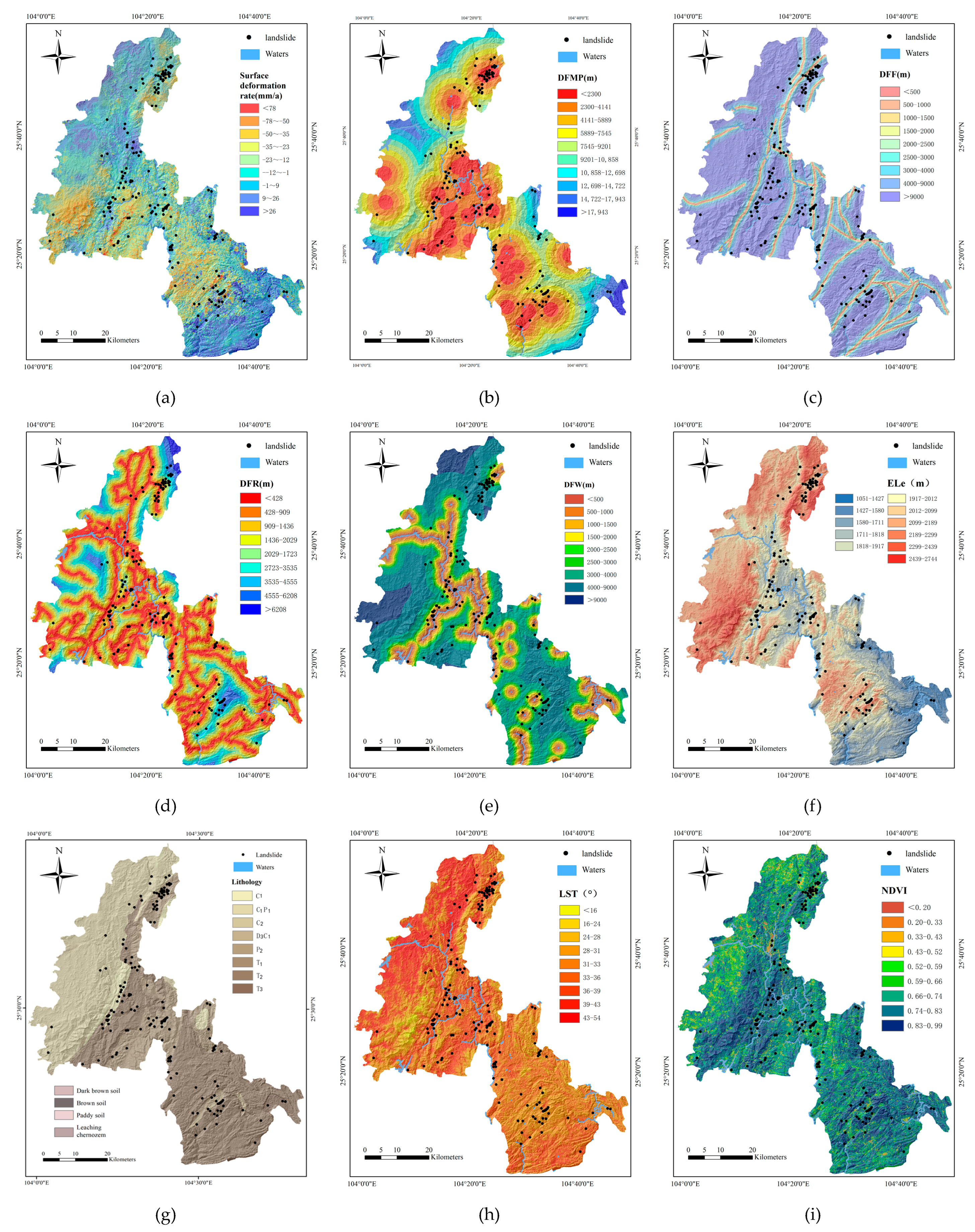
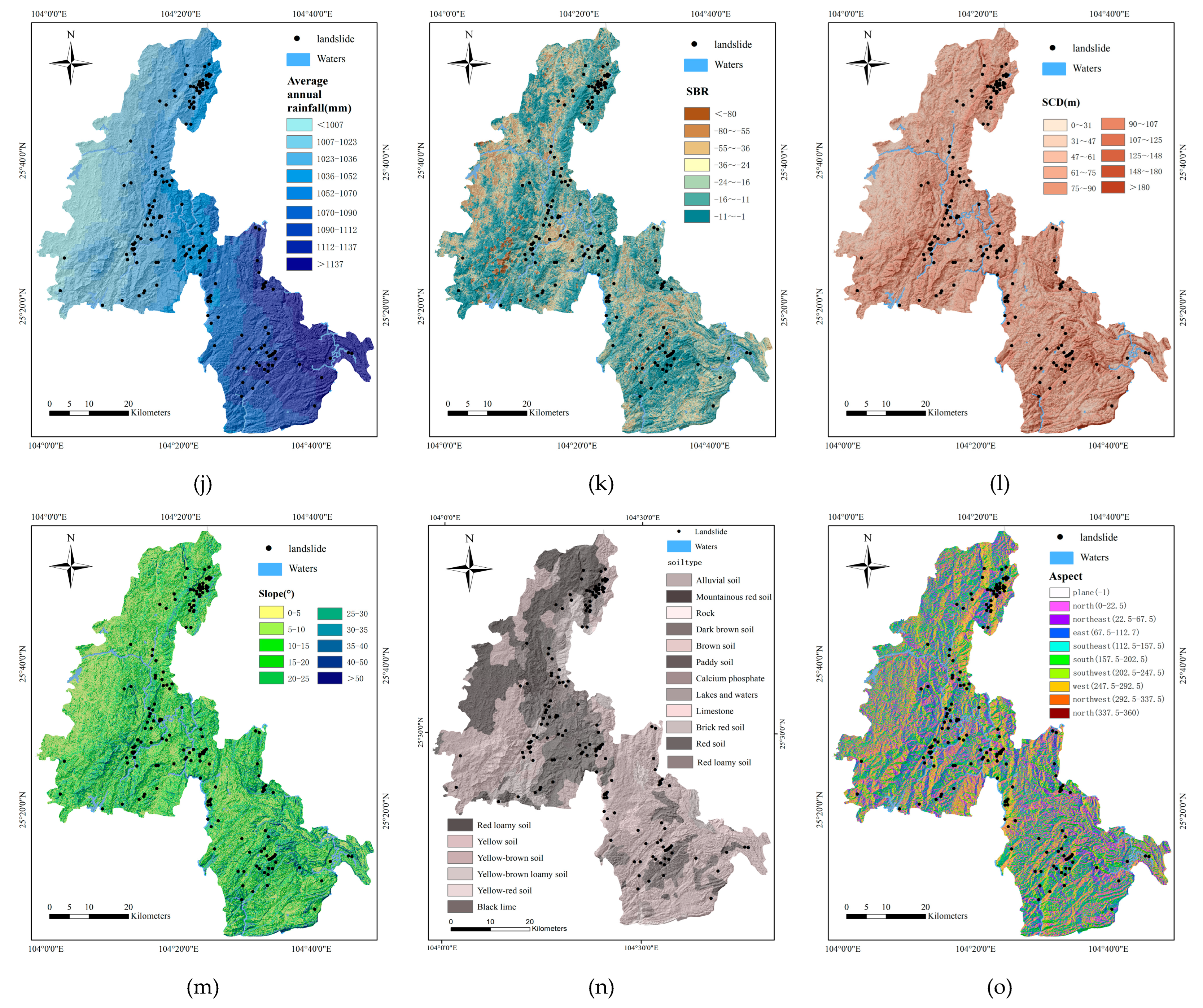
Jia et al. (2019) [37] pointed out that the factors influencing the occurrence of karst geohazards mainly include topography, geology, human activities, and carbonate distribution, and the karst geohazard sources can be categorized into topographic risk factors (elevation, slope, and surface cutting depth) and geologic risk factors (stratigraphic lithology and geologic formations) according to the analytical decomposition method (ADM), in addition to karst caves and the water circulation [38], surface subsidence phenomenon [39], anthropogenic mining activities [9], and the combined effect of natural and anthropogenic activities [40] and other influences on landslide disasters have also been mentioned. Therefore, in this paper, 17 factors were selected to construct the landslide conditioning factor system (Table 2, Figure 2).
(1) Topographic and geomorphologic factors
Topographic and geomorphologic factors include elevation (Ele) [41], surface cut depth (SCD) [3], slope (Slope), and aspect (Aspect). These factors were obtained by cropping, extracting, and analyzing ASTER GDEMV2 digital elevation data at 30 M resolution using ArcGIS 10.4 (Build 5524) software tools.
(2) Surface cover factors
Surface cover factors include soil type (ST), soil erosion modulus (SEM), soil bare rate (SBR), NDVI [31], and land surface temperature (LST). The surface cover is the material basis for landslides and other geologic disasters. Its assessment factors mainly include soil type (ST), affecting the water-holding properties and shear resistance of the soil layer [42]; soil erosion modulus (SEM), strongly correlated with landslide disasters [43]; and soil bare rate (SBR). Additionally, the nature of surface cover material and vegetation impacts the soil layer’s resistance to erosion [44] and influences the interaction between surface water and subsurface high-permeability aquifers. This interaction, in turn, affects the development of dissolution geomorphology in the subsurface carbonate layer of karst regions [45]. NDVI and land surface temperature (LST), critical indicators of vegetation behavior and change, were also considered important conditioning factors [46]. Numerous studies have focused on the effect of temperature changes on soil, primarily indicating that temperature affects processes such as soil compressibility, shear resistance, and shear strength [47,48], proving that temperature plays a role in controlling and driving slope instability. Based on Landsat-8 remote sensing data, this study calculated the soil bare rate (SBR) and NDVI values. The land surface temperature (LST) was derived using atmospheric correction methods [49], and soil erosion modulus (SEM) was calculated based on the RUSLE model [50].
In this case, the normalized vegetation index (NDVI) is calculated as follows [51]:
N D V I = ( N I R R ) ( N I R + R )
where N I R is the near-infrared band and R is the red band.
The soil bare rate (SBR) was adopted from the commonly used bare soil vegetation index (GRABS), and the formula is specified as follows:
G R A B S = V I 0.09178 × B I + 5.58959
Multiple bands of TM and OLI were transformed using the tasseled cap method into greenness ( V I ), brightness ( B I ), moisture ( W I ), and other noise components. The greenness component ( V I ) strongly correlates with vegetation cover, making it helpful in evaluating vegetation behavior. In contrast, the brightness component ( B I ) is highly correlated with bare soil and can assess bare soil conditions [52]. Therefore, the bare soil vegetation index, formed by combining B I and V I , reflects bare soil conditions more accurately.
(3) Hydrological factors
Hydrological factors include commonly used factors such as distance from water (DFW) [31], average annual rainfall (AAR) [31], and topographic wetness index (TWI) [53]. The unique hydrological environment in the region makes the karst system complex, heterogeneous, and unpredictable. Its environmental effects include river erosion on slopes, lateral erosion, and other destructive forces on the geotechnical body [54], as well as the hydrodynamic interaction between surface water and groundwater [32]. For example, Bailly-Comte et al. [55] demonstrated that the recharge capacity of surface runoff influences groundwater levels. Increased water pressure in karst channels at high water levels causes karst overflow springs to discharge, reducing the stability of rock slopes.
(4) Human activity factors
Human activity factors include distance from mining sites (DFMS) and distance from roads (DFR). The distance from mining sites is selected based on the focus of landslide disaster research in Southwest China. Mining activities in fragile geological structures cause stress concentration, rock strength decline, and deformation of the mining area [8]. Thus, studying landslide susceptibility near mining sites is crucial. This paper adds the factor of distance from mining sites to the assessment.
(5) Geological factor
Geologic factors include lithology (LI), distance from faults (DFF), and surface deformation rate (SDR). Among the karst geomorphic features, the destructive effects of underground karst development, such as cavities and fissures, have the most significant impact on landslide disasters [45]. Lithology reflects rock permeability and solubility and can also indicate the stratigraphic structure of the region. Tectonic movement is active near faults and other geological formations, leading to fractured rocks with high hydraulic conductivity [56]. These factors are essential for karst development, reflecting heterogeneous differences in karst areas. Fissures generated by the dissolution of buried soluble rocks can also destroy overlying materials. Activities such as mining can cause subsidence effects on the karst surface, increasing the tendency of inclined surfaces to tilt towards valleys or slopes [57], potentially resulting in landslides [58].
Therefore, this paper includes the surface deformation rate factor as a quantitative index of ground subsidence conditions. The specific extraction method for this factor is as follows:
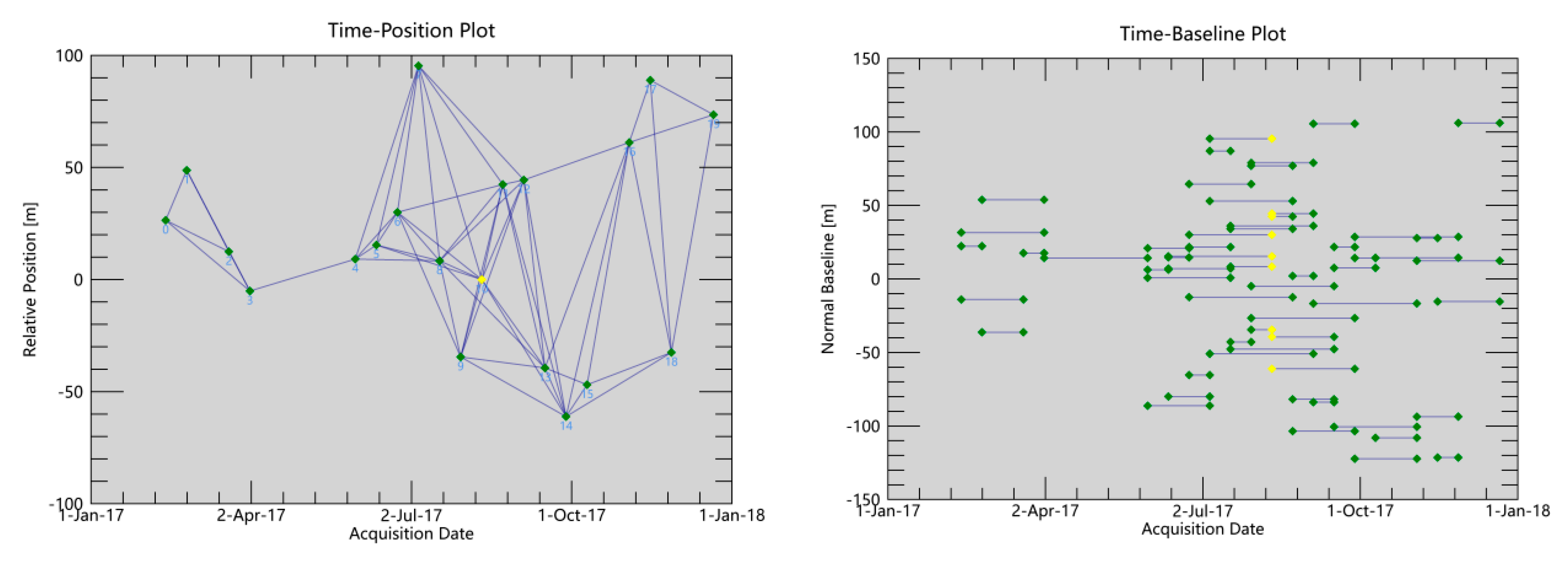
This study employs the SBAS-InSAR technique to determine the surface deformation rate in the study area from 2017 to 2018, highlighting ground subsidence trends in the karst region during this period. A total of 34 Sentinel-1A Single Look Complex (SLC) images, captured between 12 February 2017 and 21 December 2017 (Table 3), were used, with the image from 11 August 2017, designated as the super-master image. The temporal baseline threshold was set to 60 days, and the spatial baseline was established at 2% of the critical baseline length. The multi-look ratio was set to 10:2. The Minimum Cost Flow method was used for phase unwrapping, and Goldstein filtering was applied with a coherence threshold of 0.2. After discarding interferometric pairs with unsatisfactory results, orbital refinement and re-flattening were performed based on Ground Control Points (GCPs), producing the spatiotemporal baseline distribution of the interferometric pairs (Figure 3). The deformation rate in the region was estimated through two rounds of inversion, generating a deformation rate distribution map along the line of sight that retains only negative deformation rates (Figure 4). Finally, the Inverse Distance Weighting (IDW) interpolation method was used to generate a continuous raster dataset of surface deformation rates for the study area.

3. Methodology

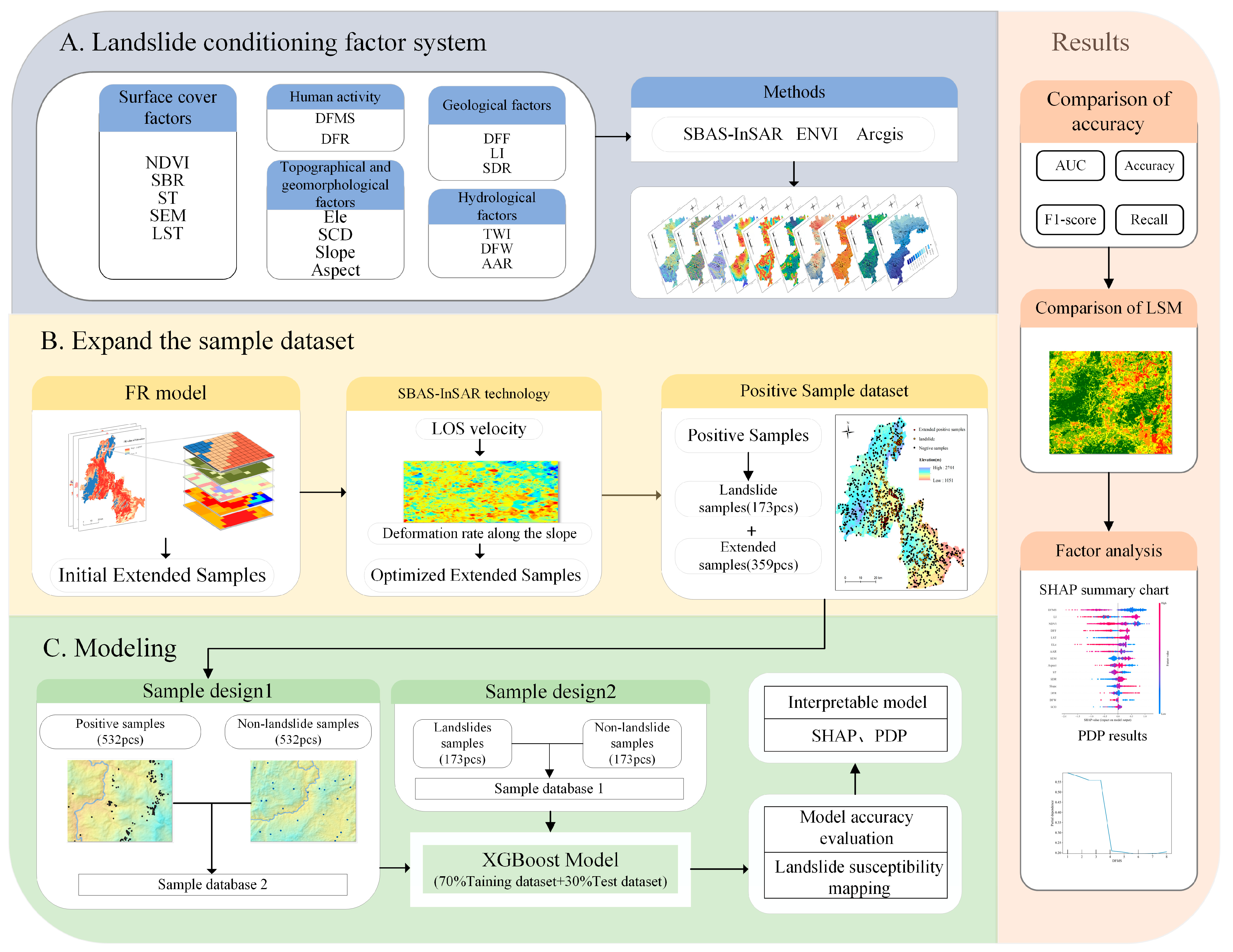
This study integrates FR and SBAS-InSAR interpretation results to enhance the landslide sample dataset. The XGBoost-SHAP-PDP algorithm is employed to develop a comprehensive interpretative framework for landslide susceptibility assessment models, enabling a comparison of results before and after sample expansion. The methodological framework of this study comprises four key components, as illustrated in Figure 5: (1) Construction of the landslide susceptibility conditioning factor system: This includes selecting and processing factors. Seventeen factors were selected from five categories: topographical and geomorphological factors, geological factors, surface cover factors, human activity factors, and hydrological factors. (2) Expansion and optimization of the sample dataset: A strategy combining frequency ratio (FR) and SBAS-InSAR technology interpretation results was employed for sample dataset expansion and optimization. (3) XGBoost machine learning algorithm and SHAP-PDP interpretable algorithm were used to construct the landslide susceptibility evaluation model. The data were randomly divided into training and validation sets in a 7:3 ratio to facilitate the machine learning process and generate LSM diagrams. (4) Result analysis: This includes accuracy testing, comparison, and interpretability analysis. The accuracy of the two models, before and after sample expansion, was compared based on results from ROC curves, AUC values, precision, and recall rates. Additionally, the primary contributing factors of landslide disasters and some influencing mechanisms were analyzed using SHAP summary plots, factor importance ranking plots, and PDP partial dependence plots.

3.1. Frequency Ratio Method

Frequency Ratio (FR) is a single-factor quantitative analysis method [28], which determines the degree of influence of each factor on landslide disaster at different intervals by calculating the density and frequency ratio of the distribution of landslides at different grading intervals of the conditioning factor. The formula for FR is:
F R = F j / F C j / C
where, F j represents the count of geohazard rasters in classification interval j for the factor; F denotes the total geohazard rasters in the interval; C j indicates the count of rasters in classification interval j for a factor; and C is the overall number of rasters in the study area.
When FR > 1, the classification interval of the conditioning factor exerts a significant influence on landslide occurrence, indicating high susceptibility; conversely, when FR < 1, it denotes low susceptibility [15,59]. In this study, the Frequency Ratio (FR) method is employed to calculate the FR values for each interval of every factor. An FR value attribute dataset is established based on raster cells, and a positive and negative expansion sample set is created by categorizing according to the FR threshold.

3.2. SBAS-InSAR Technology

The Small Baseline Subset InSAR (SBAS-InSAR) technique, initially proposed by Berardino and Lanari [60], involves selecting interferometric pairs from acquired SAR images based on temporal and spatial baselines that meet certain thresholds. These pairs are grouped into subsets according to baseline conditions to maximize the coherence of the interferometric phases. The differential interferograms generated from these pairs undergo filtering and deconvolution to enhance coherence. High-coherence points are then identified, and the interferograms are further refined to remove elevation phases, atmospheric errors, and noise. Through an iterative process, the actual deformation phases are extracted. The time series and deformation rates for each subset are determined using the least squares method, and multiple small baseline sets are resolved together through Singular Value Decomposition (SVD), which increases the time sampling frequency [39,61]. This method addresses issues like decorrelation and atmospheric effects caused by spatio-temporal baselines in the D-InSAR technique, making it suitable for long-term deformation analysis [62]. The specific principles are as follows:
Assuming that there are ( N + 1 ) frames of repeat-pass SAR images with time series t 0 , t 1 , t 2 , …, t n in a particular area, and certain temporal and spatial baseline thresholds are set. According to the interferometric baseline combination rule, M frames of differential interferograms are formed under short baseline spacing conditions, satisfying:
N + 1 2 N N ( N + 1 ) 2
The ith interferogram (0 < i < M ) generated from the two images at times t A and t B can be expressed as the interferometric phase of the image element ( x , r ) after removing the influence of orbit error, leveling effect, and terrain phase:
φ A , B i ( x , r ) = φ d e f i ( x , r ) + φ t o p o i ( x , r ) + φ a p s i ( x , r ) + φ o r b i ( x , r ) + φ n o i s e i ( x , r )
where φ d e f i ( x , r ) is the line-of-sight deformation corresponding to t A - t B , φ t o p o i ( x , r ) is the terrain phase error, φ a p s i ( x , r ) is the atmospheric phase error, φ o r b i ( x , r ) is the phase error due to the baseline orbit, and φ n o i s e i ( x , r ) is the noise error.
Since M multi-view differential interferograms are formed, M equations can be derived according to Equation (2), which can be represented in matrix form as follows:
δ φ ( x , y ) = A φ ( x , y )
A is an M × N matrix, with each row corresponding to an interferogram and each column corresponding to a SAR data view. The matrix A depends on the interferograms generated from the dataset. If all datasets belong to a single small baseline subset ( L = 1), then M N , making A a regular N-rank matrix. In this case, the estimate can be solved using the least squares method, calculated as follows:
ϕ ^ ( x , y ) = ( A T A ) 1 A T δ ϕ ( x , y )
However, the scenario of a single subset is rare; typically, the dataset is distributed across multiple subsets ( L > 1). This situation results in A being a singular matrix with a rank of N L + 1 . Consequently, the system of equations has an infinite number of solutions. To address this, the Singular Value Decomposition (SVD) method is introduced to combine the multiple baseline sets and find a unique least squares solution [40], thereby obtaining the cumulative deformation, i.e., the deformation time series over the entire period. However, the cumulative deformation may exhibit temporal discontinuities. The interferometric phase is expressed as the product of the average deformation rate and the time interval between the acquisition of two neighboring SAR images to obtain a more physically meaningful settlement sequence. Assuming the deformation rate between the k -th and ( k + 1 )-th interferograms, the cumulative deformation between t A and t B can be expressed as:
δ φ d e f ( x , r ) = 4 π λ k = t A t B 1 v k , k + 1 ( t k + 1 t k )
where λ is the radar wavelength, and the deformation rates at different SAR acquisition moments can be obtained by three-dimensional spatio-temporal phase unwrapping of the N -amplitude interferometric fringe pattern.
The deformation rate information obtained at this stage represents only a one-dimensional projection along the satellite imaging line of sight in the three-dimensional motion direction of the actual surface. To minimize the differences in the deformation rate inversion results due to variations in surface geometry and satellite line-of-sight angle, the annual average deformation rate at all acquisition points must be projected onto the slope gradient direction [63,64]. The equations are as follows:
V s l o p e = V L O S C
C = cos β
cos β = ( sin a cos φ ) ( sin θ cos α s ) + ( cos a cos φ ) ( sin θ sin α s ) + sin φ cos θ
β denotes the angle between the radar satellite line-of-sight direction and the slope direction, a denotes the slope direction, φ denotes the slope gradient, θ denotes the satellite incidence angle, and α s denotes the angle between the satellite's orbital direction and the due north direction.
During the calculation process, V s l o p e will tend to infinity when the value of β is near 90°, i.e., when the value of cos β is near 0. Therefore, in order to avoid a very large anomalous solution in absolute value during the conversion process, Herrera [65] et al. used the empirical value of cos β = ±0.3 as a fixed threshold, and set cos β = −0.3 when −0.3 < cos β < 0, and cos β = 0.3 when 0 < cos β < 0.3.

3.3. XGBoost Algorithm

XGBoost (Extreme Gradient Boosting) is an ensemble machine learning algorithm proposed by Chen and Guestrin in 2016 [66]. It is based on decision tree ensembles and uses the gradient boosting algorithm to fit the residuals between the predicted values of previously generated decision trees and the actual data [67]. By iteratively generating new decision trees in the direction of the gradient descent of the previous tree’s loss function, XGBoost updates weak learners to strong learners, thereby improving overall predictive accuracy and enhancing the model’s generalization capability. In this study, the XGBoost model is employed to assess landslide susceptibility in karst areas, resulting in a landslide susceptibility map and yielding satisfactory predictive outcomes [13].
For a given dataset with n examples and m features D = { ( x i , y i ) } ( | D | = n , x i R m , y i R ) , a tree ensemble model uses K additive functions to predict the output. For the ith sample x i the landslide prediction result is expressed as y ^ i , then the expression is as follows [66]:
y ^ i = ϕ ( x i ) = k = 1 K f k ( x i ) , f k F
where F = { f ( x ) = w q ( x ) } ( q : R m T , w R T ) is the space of regression trees (also known as CART). Here, q represents the structure of each tree that maps an example to the corresponding leaf index. T is the number of leaves in the tree. Each f k corresponds to an independent tree structure q and leaf weights w . The results of the model’s evaluation of the sample landslide susceptibility are obtained by summarizing the corresponding sample leaf node weights w in the CART.
To learn the set of functions used in the model, we minimize the following regularized objective.
L ( ϕ ) = i l ( y ^ i , y i ) + k Ω ( f k )
Ω ( f ) = γ T + 1 2 λ | | w | | 2
where i l ( y ^ i , y i ) and k Ω ( f k ) are for the model loss function and regular term respectively, the larger the value of the regular term represents the more complex the model; y ^ i is the model prediction result, y i is the true value of the sample. γ and λ are constants.
The gradient boosting strategy is used in the model training, assuming that the prediction result of the ith sample in the tth round of iteration is y ^ ( t ) , f t ( x i ) is the newly introduced regression tree, and the objective function can be obtained by derivation as:
L ( t ) = i l ( y i , y ^ ( t 1 ) + f t ( x i ) ) + Ω ( f k ) + c o n s t a n t

3.4. SHAP Algorithm

SHAP (Shapley Additive exPlanation) is a method proposed by Lundberg and Lee [68] to interpret black-box models. Derived from coalitional game theory, it is used to interpret the prediction results of various classification and regression models, particularly the decision-making processes of complex black-box models. Therefore, applying the SHAP method for interpretability analysis helps explore key factors influencing landslide occurrences and the extent of their impacts [69]. The specific calculation formula is shown in Equation (3), i.e.:
f ( x i ) = ϕ 0 ( f , x ) + j = 1 k ϕ j ( f , x i )
where f ( x i ) is the predicted value of the ith sample input to the model; x i is the input variable; ϕ 0 ( f , x ) is the explanatory model constant calculated by the model, i.e., the predicted mean value of all training samples; and ϕ j ( f , x i ) is the contribution value of the jth evaluation factor. A positive SHAP value indicates that the factor makes a positive contribution to landslide development.

3.5. PDP Algorithm

Partial Dependence Plot (PDP) is a global interpretation method showing the marginal effects and overall influence of one or two conditioning factors on a machine learning model’s prediction results. It presents low-dimensional graphical representations of the prediction function, displaying the relationship between individual conditioning factors and prediction outcomes [70]. Therefore, the PDP method can analyze the impact of primary contributing factors on landslide occurrences.
The principles of the PDP algorithm are as follows:
f ^ x s ( x s ) = E x s [ f ^ ( x s , x c ) ] = f ^ ( x s , x c ) p c ( z c ) d z c
x s is the factor to be interpreted; x c is the other factor, and x s and x c together form the entire factor space X.
f ^ x s ( x s ) = 1 n i = 1 n f ^ ( x s , x i , c )
Equation averages the effect of other feature factors in the model by marginalizing x c on the basis of the training dataset. The mean f ^ x s ( x s ) of the predicted results of the model output at all possibilities of x c when x s takes a fixed value to obtain the relationship between the feature factor x s to be explained and the predicted results of the machine learning model.

3.6. Sampling Strategies

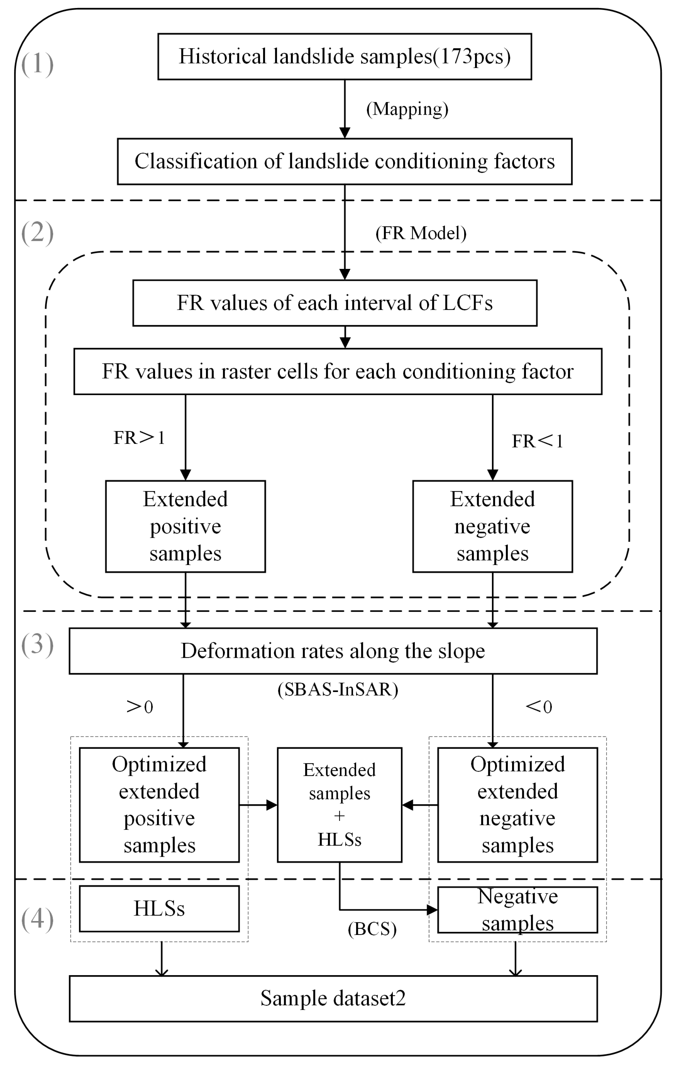
To assess the sample expansion strategy’s effectiveness, this paper constructs two sample datasets for landslide susceptibility assessment: one before and one after sample expansion. Firstly, sample dataset 1 is created using the traditional method, maintaining a 1:1 ratio of historical landslide samples to non-landslide samples. Additionally, sample dataset 2 is developed by implementing an optimization strategy that combines the frequency ratio (FR) method with SBAS-InSAR interpretation results to supplement the landslide samples. The technical roadmap is illustrated in Figure 6.
The process includes the following steps:
(1)
Calculate the frequency ratio (FR) value for each interval of each conditioning factor to obtain an FR value attribute dataset based on raster cells.
(2)
Create an initial expansion sample set based on FR values. Filter samples using geographic environment indicators: select raster cells with a minimum FR value greater than 1 as expansion positive samples, totaling 955; select raster cells with a maximum FR value less than 1 as expansion negative samples, totaling 99.
(3)
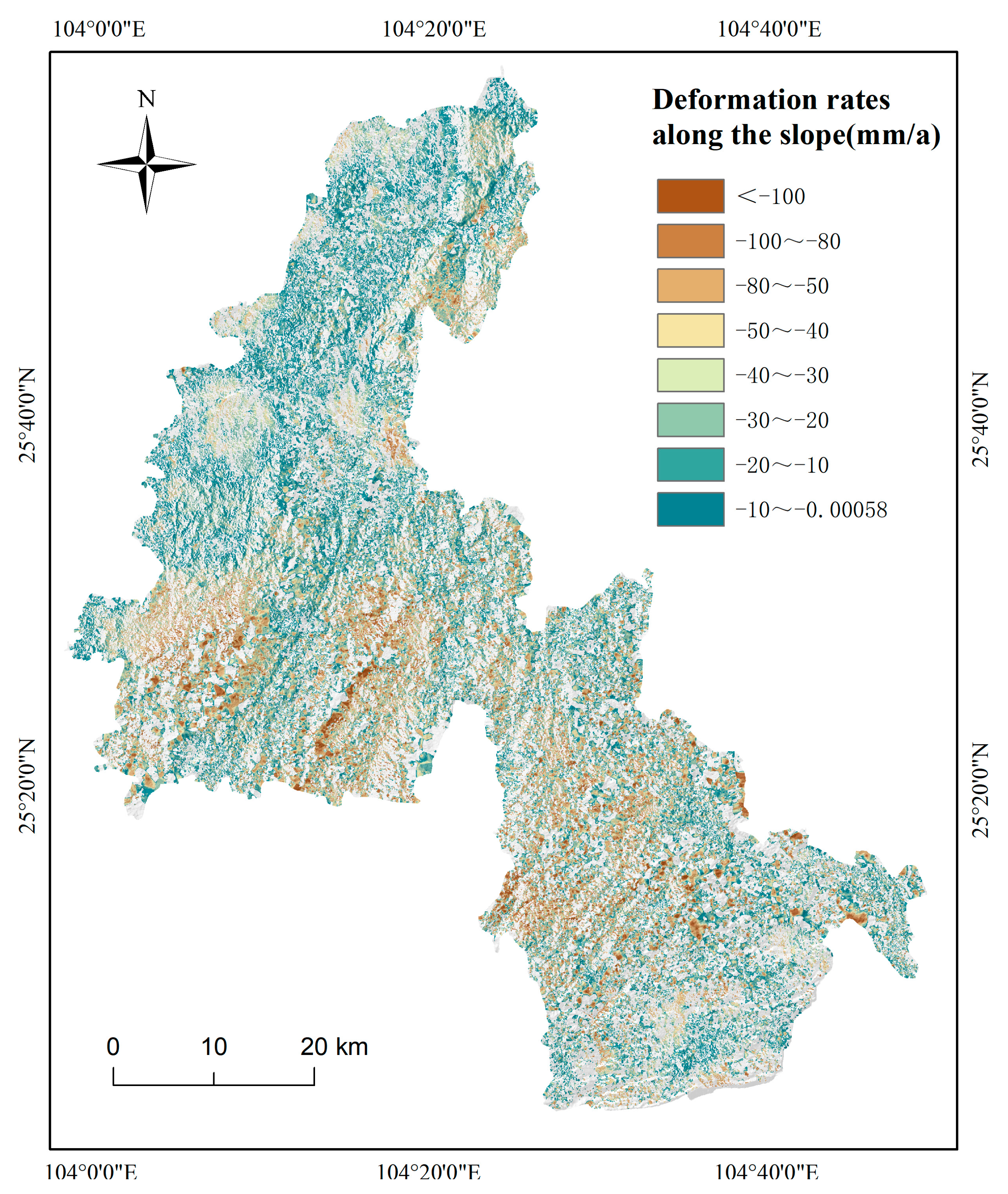
Use the deformation rate along the slope direction obtained by SBAS-InSAR technology to refine the expanded sample dataset. The deformation rate along the line of sight (LOS) of the satellite imaging is initially deduced using SBAS-InSAR technology. However, there is some bias between this deformation information and the actual surface deformation. Therefore, the LOS deformation rate is converted to the slope direction deformation rate using a relevant formula and interpolated in ArcGIS with the inverse distance weighting method. Only negative deformation rate values are retained to obtain the final deformation rate distribution along the slope direction (Figure 7). If the deformation rate along the slope direction is less than 0, it indicates deformation in that direction; if greater than 0, it indicates no deformation. Considering surface spatial deformation factors fully, the final expanded positive samples are those with slope direction deformation rates less than 0, totaling 359, and the final expanded negative samples are those with deformation rates greater than 0, totaling 16.
(4)
The buffer-controlled sampling (BCS) method was used to generate random non-landslide samples. These samples, along with the expanded set of positive and negative samples and historical landslide samples, were merged to achieve a 1:1 ratio of landslide to non-landslide samples. This process created the final dataset.

4. Results

4.1. Models’ Performance Test and Comparison

4.1.1. Confusion Matrix

Landslide susceptibility is a typical binary classification problem [13]. Model accuracy can be quantitatively assessed using Accuracy, Precision, Recall, and F1_score values, which range from 0 to 1. Higher values denote greater model accuracy. The formula for each indicator is as follows:
A c c u r a c y = T P + T N T P + F P + T N + F N
P r e c i s i o n = T P T P + T N
Re c a l l = T P T P + F N
F 1 _ s c o r e = 2 P r e c i s i o n × R e c a l l P r e c i s i o n + R e c a l l
In the formula, True Positive (TP) indicates that both actual and predicted values are positive; True Negative (TN) suggests that the model correctly predicts negative category samples as negative categories; False Positive (FP) indicates that the model incorrectly predicts negative category samples as positive categories; and False Negative (FN) suggests that the model incorrectly predicts positive category samples as negative categories.
This study employs the confusion matrix along with accuracy, precision, recall, and F1_score metrics to evaluate model performance (Table 4 and Table 5). By comparing the performance indicators of the confusion matrix before and after sample expansion, a substantial improvement in each indicator is observed. This indicates that the sample expansion strategy, which combines the frequency ratio (FR) with SBAS-InSAR interpretation results, results in higher prediction accuracy and reliability.

4.1.2. ROC Curve and AUC Value

The Receiver Operating Characteristic (ROC) curve is a commonly utilized metric for assessing the accuracy of landslide susceptibility predictions. In the ROC curve, the y-axis represents the true-positive rate, indicating the probability of correctly predicting disaster points, while the x-axis represents the false-positive rate, indicating the probability of incorrectly predicting non-disaster points. The area under the ROC curve (AUC) measures the model’s effectiveness, with values ranging from 0 to 1. A value of 0 indicates a meaningless model, thus the closer the AUC value is to 1, the higher the model’s prediction accuracy.
To evaluate the effectiveness of the sample optimization strategy, this study employed the XGBoost algorithm to train landslide susceptibility models using both the initial and expanded sample datasets. The models’ accuracies were assessed and compared by analyzing their ROC curves and AUC values (Figure 8). The results showed that the AUC values for the training and testing sets of the landslide susceptibility assessment model using the initial sample dataset were 0.8921 and 0.9544, respectively. Using the expanded sample dataset, the AUC values for the training and testing sets improved to 0.9579 and 0.9790, respectively.
Comparative analysis indicates that the sample expansion strategy combining the frequency ratio (FR) and SBAS-InSAR interpretation results significantly enhances model accuracy and optimizes performance, as evidenced by the substantial increase in AUC values for the expanded sample models.

4.2. Comparison of Landslide Susceptibility Mapping

The XGBoost model was trained to predict landslide susceptibility within the study area (Figure 9). Using the natural breaks classification method, susceptibility was categorized into five classes: very high, high, medium, low, and very low. Landslide susceptibility maps were generated for both the initial and expanded sample datasets. Based on the training results, the number of landslides and raster cells within each susceptibility class were counted. The area proportion and landslide density for each class were calculated. The results before and after sample expansion are shown in Table 6.
The data show that before sample expansion, low and very low susceptibility areas accounted for 51.483% of the total area, but only 9.249% of the total landslide points. High and very high susceptibility areas accounted for 25.157% of the total area but 78.612% of the total landslide points, with a landslide density of 0.289149 landslides/km2 in very high susceptibility areas. It is evident that high and very high susceptibility zones were overrepresented, and the landslide density in very high susceptibility zones was relatively low. Considering the prediction accuracy results from Section 4.1, it can be inferred that there may be deficiencies in the evaluation process, leading to reduced model accuracy. These issues may stem from the evaluation factors, sample data quality and quantity, and modeling methods.
After sample expansion, low and very low susceptibility areas comprised 72.539% of the total area but contained only 12.139% of the landslides. Conversely, high and very high susceptibility areas covered 12.025% of the area yet accounted for 68.208% of the landslides, with a landslide density of 0.436809 landslides/km2 in very high susceptibility zones. The proportion of areas in each susceptibility level is more reasonable after sample expansion, and the landslide density in each level is higher than before. Thus, both models are dependable, but the evaluation results and prediction accuracy of the model after sample expansions are significantly higher. Therefore, the sample optimization strategy combining the FR method and SBAS-InSAR technology is crucial for improving the accuracy of LSM in karst areas.
The results after sample expansion show that high and very high susceptibility areas are concentrated in regions below 2000 m in elevation, where faults are relatively developed, and rivers are well formed. The strata in these areas are predominantly Permian, consisting of alternating layers of sandstone, shale, limestone, and interbedded coal seams. These areas experience significant human activity, including coal mining and road construction, resulting in low vegetation cover. Consequently, the stability of slopes is reduced under rainfall, making landslides more likely.

4.3. SHAP Interpretability Results

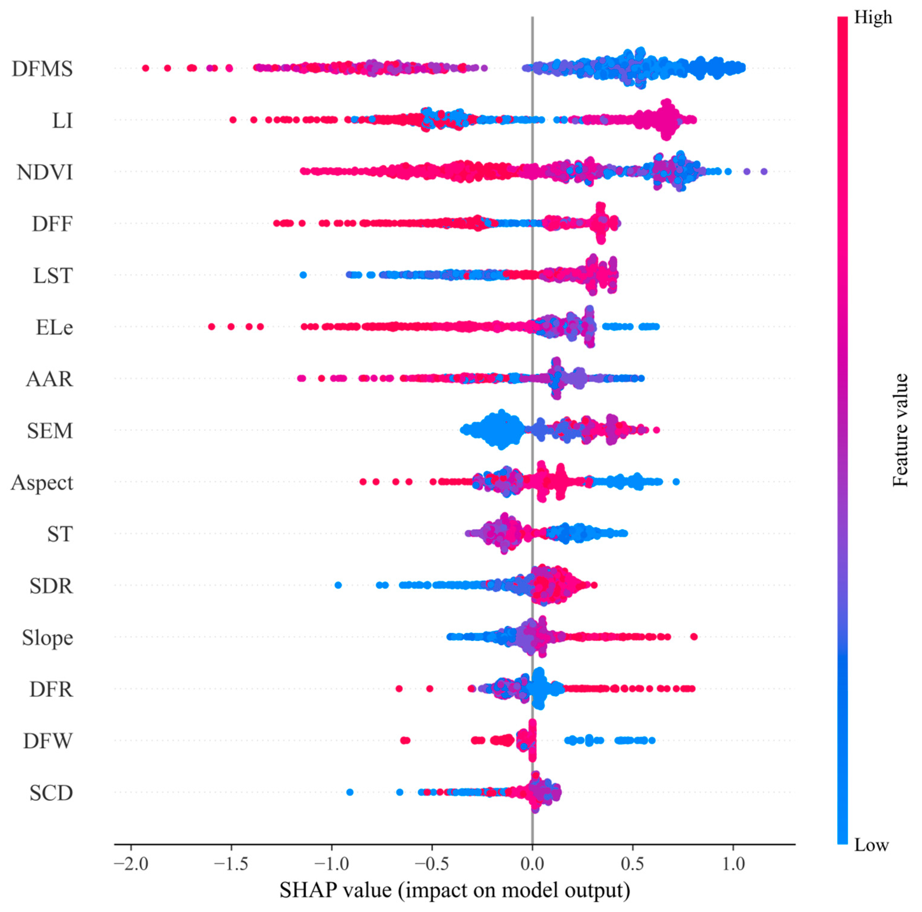
This paper presents a summary plot using the SHAP algorithm (Figure 10) to quantify each factor’s contribution and importance to the model’s predictions from a global perspective through Shapley values. Each point in the graph represents a sample and displays the size of the feature value as well as its corresponding SHAP value. Points are colored according to the size of the factor value, with larger values shown in red. A positive SHAP value signifies that the feature positively influences landslide occurrence, with larger SHAP values indicating greater contribution.
The summary plot shown in the figure is based on the landslide susceptibility model after sample expansion. The selected factors significantly contribute to the occurrence of landslides and exhibit certain patterns. For instance, the SHAP values for factors such as distance from mining sites and NDVI increase as the feature values decrease.
By averaging and organizing the SHAP values of all samples, a factor importance ranking plot (Figure 11) can be obtained, allowing for a visual comparison of each factor’s contribution. From the factor importance ranking plot, the distance from mining sites, lithology, and NDVI are ranked in the top three, with average SHAP values all greater than 0.4.
Additionally, factors such as land surface temperature, distance from faults, elevation, average annual rainfall, soil erosion modulus, aspect, soil type, and surface deformation rate are also strongly correlated with landslide occurrence, each with an average SHAP value greater than 0.1. In contrast, factors like distance from water and soil bare rate are ranked lower and have a lesser influence on landslide occurrence.

5. Discussion

5.1. Effectiveness of Combining FR and SBAS-InSAR Sample Extension Strategies

The efficacy of machine learning models hinges on the quality and volume of their sample datasets. Owing to the limited landslide samples in the Eastern Yunnan Karst region, the quantity, and quality of non-landslide samples are usually constrained by the availability of landslide samples. This limitation hinders the model from obtaining representative feature information, thus affecting the training efficacy and prediction accuracy of LSM. Therefore, augmenting the quantity of training samples in areas with limited samples is a crucial method to enhance the accuracy of LSM [50].
In this study, the sample expansion strategy, based on the frequency ratio (FR) method, establishes an FR value attribute dataset by calculating the FR values of all conditioning factors for each interval and filtering them using one as the FR value threshold. This method ensures that the expanded positive samples fall within the intervals of higher landslide susceptibility for each conditioning factor, effectively addressing the imbalance between positive and negative samples caused by limited data. On this basis, the surface deformation rate information obtained through SBAS-InSAR technology is utilized to further refine the extended sample set, fully considering geospatial deformation factors to reduce the false-positive and false-negative rates of the samples.
Surface spatial deformation characteristics are crucial in the study of landslides and related disasters, especially in areas characterized by karst topography where ground subsidence is common. The subtle surface deformation caused by ground subsidence significantly impacts surface stress redistribution and slope stability. Therefore, the sample expansion strategy proposed in this paper, which combines frequency ratio (FR) and SBAS-InSAR interpretation results, simultaneously addresses the effects of geo-environmental indicators and geospatial deformation factors on sample quality and model outcomes. This strategy not only reduces the error in negative sample selection but also increases the sample size, resulting in a more comprehensive feature information dataset. It offers the advantages of simplicity, ease of calculation, and strong interpretability.
Meanwhile, the model accuracy and landslide susceptibility mapping results before and after sample expansion demonstrate significant improvements in assessment metrics such as AUC, F1-score, precision, recall, and accuracy. This indicates that the sample optimization strategy, combining frequency ratio (FR) and SBAS-InSAR technology interpretation results, can effectively enhance the accuracy and reliability of landslide susceptibility assessment models.

5.2. Analysis of the Primary Contributing Factors of Landslide Susceptibility in Karst Landscapes Based on SHAP Modeling

The SHAP interpretable model ranked the importance of factors, revealing that distance from mining sites (DFMS), lithology (LI), and NDVI were the most critical for landslide occurrence. First, lithology is a crucial control parameter in slope stability [40]. The stratigraphy of the landslide-prone area is primarily composed of formations from the Permian and Carboniferous periods. The lithology includes dolomite, graywacke, sandstone, and mudstone, with interspersed layers of coal and volcanic rocks. Dolomite and greywacke, categorized as carbonate rocks, are widely distributed in karst areas, and their lithological characteristics are strongly associated with landslide occurrences. Due to the fragile and soluble nature of karst mountainous areas, features such as cavities, voids, dissolution cracks, differential erosion, and filled caves are widely developed [71]. El-Haddad et al. [72] identified and analyzed five different landslide mechanisms in carbonate cliffs and slopes, including rock decomposition due to differential erosion, dissolution along large fissures, and rupture of caves in carbonate slopes, all indirectly related to karst features. The distance from mining sites was ranked as the most important factor, with mining activities being highly related to landslide disasters in the karst region of eastern Yunnan. In summary, the fragile lithological characteristics of the karst region amplify the destructive effects of human engineering activities, such as mineral extraction and infrastructure development, making landslide disasters more common in these areas. Additionally, there is a close relationship between NDVI and landslides [73]. Surface vegetation provides a protective effect on slopes, directly affecting soil erosion and slope modification [74]. The plant root system can also enhance the shear strength and seepage resistance of slopes, reducing the probability of landslides.
From a macroscopic perspective, factors affecting landslide occurrence can be classified into two categories: geographic environmental conditions and triggering conditions [75]. The synergistic influence of these factors precipitates landslide occurrences. The former pertains to terrain and environmental conditions with minimal changes over long periods, including static factors such as lithology, soil type, elevation, and surface cutting depth. The latter refers to natural or human-induced damage-triggering factors, such as precipitation fluctuations, earthquakes, and human activities. Relevant factors in this paper include distance from mining sites, average annual rainfall, and distance from roads. The surface deformation rate is also a triggering condition factor, reflecting the intensity and trend of surface deformation. The SHAP interpretable model results show that geo-environmental condition factors (lithology, NDVI, land surface temperature) dominate among the top five conditioning factors. Additionally, triggering condition factors such as distance from mining sites and faults also rank in the top five, indicating the significant impact of human activities. Research reveals that human activities and urban expansion have emerged as primary drivers of landslides in recent decades, contributing to approximately 70% of landslides in China [76]. Therefore, in disaster prevention and control in high-susceptibility areas of landslides in karst landscapes, government departments should focus on the combined impact of natural and human factors and take effective measures to reduce potential losses.
Additionally, the soil erosion modulus, surface deformation rate, and land surface temperature factors introduced in this paper strongly correlate with landslide occurrence. Previous studies have less considered the influence of these factors on landslide susceptibility. Their introduction can quantitatively characterize the regional influence on landslide triggering and provide important references for constructing a landslide susceptibility assessment system in karst landscapes.

5.3. Impact Analysis of Significant Contributing Factors Based on PDP Modeling

Based on the Partial Dependency Plot (PDP), the connection between individual conditioning factors and landslide susceptibility can be further explored to analyze the influence of these factors within their variation ranges. Considering that the PDP algorithm shows both the marginal and overall effects of factors on prediction results, this study focuses on analyzing the trends and threshold effects of the PDP curves to mitigate the interference from the interactions of multiple factors. This study conducts PDP analysis on four significant factors—distance from mining sites, NDVI, land surface temperature, and surface deformation rate—to explore their influence on landslide occurrences.

5.3.1. One-Factor Dependence Analysis of Distance from Mining Sites

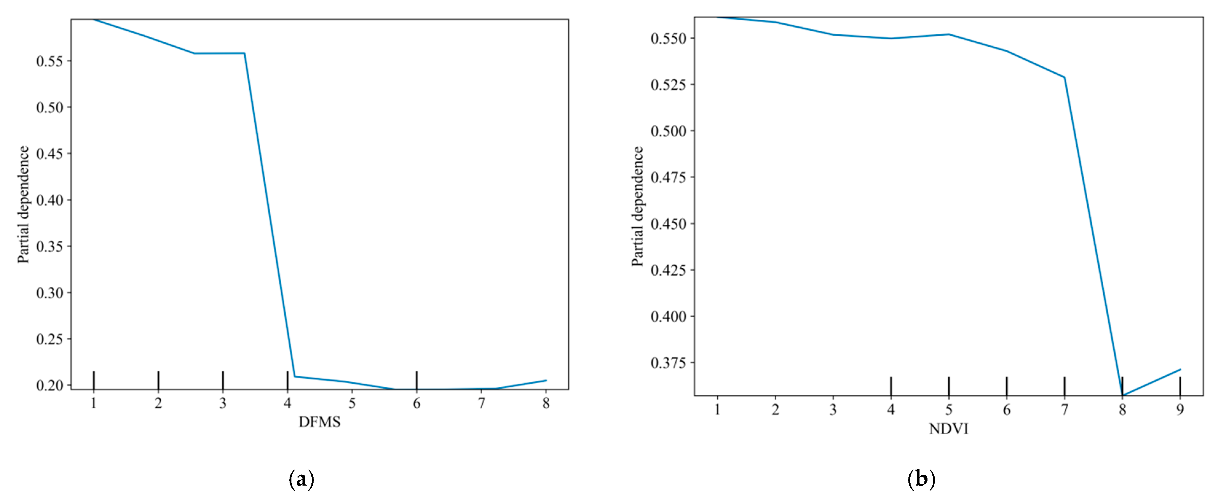
The partial dependence plot of the distance from the mining sites factors in Figure 12a shows a nonlinear negative correlation with the prediction results, indicating varying influence across different intervals. The predicted mean value of landslide incidence is remarkably high for distances less than 6000 m from the mining sites and remains relatively flat despite a decreasing trend. This indicates a higher probability of landslides within this range, while variations in factor values exert minimal influence. In the range of 6000 to 8000 m, the predicted mean value decreases sharply, implying that increased distance from the mining sites significantly inhibits landslide occurrence, indicating a reduced contribution from mining activities. Additionally, this stage shows a significant threshold effect, suggesting a critical value in this range beyond which the impact of geoturbation from mining activities decreases dramatically, leading to a significant drop in predicted mean values. For distances greater than 8000 m from the mining sites, the predicted average value remains low and stable, indicating minimal influence from mining activities on landslide occurrence. This is likely due to the reduced direct impact on the geological structure, allowing the geological body to stabilize.
The mining industry is well-developed in eastern Yunnan, but stress fluctuations from underground mining accelerate uneven settlement of the overlying strata, leading to the expansion of karst fissures and rock base rupture, which are prone to triggering landslides [7]. Due to the complex geological environment, unclear damage mechanisms, and rapid movement of landslides, mining-induced landslides are prone to causing significant losses and are a major focus of landslide disaster research in eastern Yunnan. This study proves that mining activities in karst areas significantly promote landslide occurrence, providing a reliable basis for assessing landslide susceptibility in karst regions of Southwest China.

5.3.2. One-Factor Dependence Analysis of NDVI

According to Figure 12b, the partial dependence plot curves for the NDVI factor can be roughly divided into three ranges: high value, sharp decline, and low value, all showing a general nonlinear negative correlation. When the NDVI value is below 0.6, the predicted mean value remains high, with a slow decreasing trend, suggesting a significant likelihood of landslide occurrence. However, increased vegetation cover in this range has a limited inhibitory effect on landslides, likely because the vegetation has yet to reach sufficient density and depth to stabilize the soil and significantly reduce erosion. When NDVI values are between 0.6 and 0.8, the predicted mean values decrease sharply with increasing vegetation cover, indicating that the inhibitory effect of vegetation on landslide occurrence becomes significant in this range. This range also exhibits a significant threshold effect, where reaching a certain level of vegetation cover significantly enhances soil stability and reduces landslide risk. When the NDVI value exceeds 0.8, the predicted mean value remains low and stable, indicating that within this range, changes in vegetation cover have a minimal effect on landslide incidence. This may be because the vegetation cover exceeds a critical value, making further increases have a limited impact on landslides. Other factors, such as the instability of the karst region’s lithology or the distribution of fault zones, might destabilize slopes. These findings provide important insights for the control and mitigation of landslide hazards.

5.3.3. One-Factor Dependence Analysis of Surface Deformation Rate

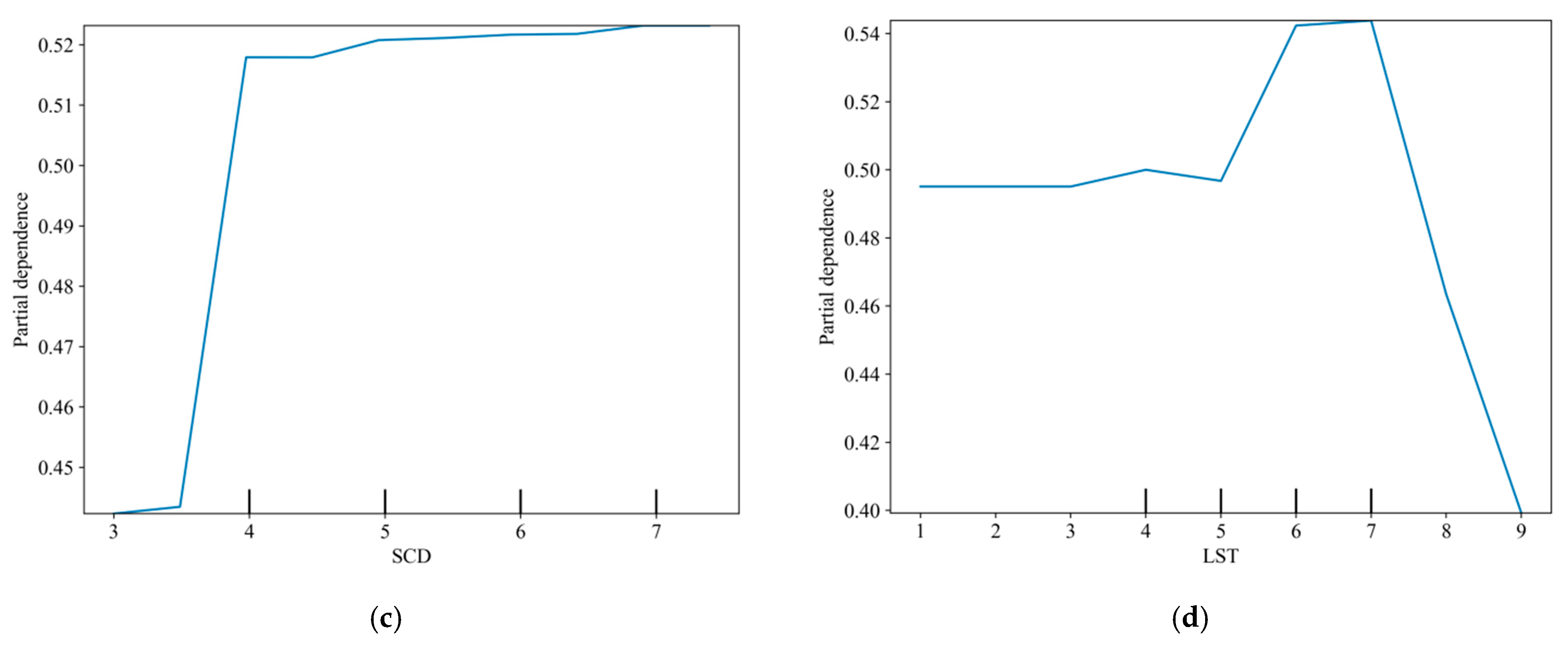
From the partial dependence plot in Figure 12c, it is evident that the surface deformation rates obtained by SBAS-InSAR technology are concentrated between −50 and 0 mm/a. The surface deformation in the area is divided into positive and negative deformations, with vector solution rate values less than zero indicating ground subsidence. An interpretive analysis of the surface deformation rate is performed using partial dependence plots, focusing on the influence of negative ground subsidence on landslide occurrence. Figure 12c illustrates the nonlinear relationship between surface deformation rate values and predicted mean values. For surface deformation rate values less than −45 mm/a, the predicted mean values are lower, due to the small number of rasters in this range. The lower probability of landslide occurrence in areas with larger surface deformation rates may be due to rapid deformation leading to quick stress release, reducing geohazard occurrence probability. Rapid subsidence or uplift may also compact soil and rock, increasing stability. To rationally explain the results of this study, more surface deformation-related landslide susceptibility research is expected in the future.
When the surface deformation rate is between −35 and −20 mm/a, the PDP curve shows a significant upward trend, indicating that changes in this range significantly affect landslide occurrence. When the surface subsidence rate is between −20 and 0 mm/a, the PDP curve is nearly flat, but the predicted mean value remains high. We hypothesize that the primary cause is the slow ground subsidence in this region, combined with the over-representation of statistical data, which results in elevated predicted mean values within this range. We disregard the high predicted values and focus on analyzing the trend and smoothness of the curve. It is evident that changes in surface deformation rate in this range exert a minimal influence on landslide occurrence. In this study, the surface deformation rate, as a special dynamic conditioning factor, performs well in landslide susceptibility assessment. It is also a meaningful factor reflecting the present state and progression of ground subsidence within the region [77], and provides a basis for optimizing its application in landslide susceptibility studies.

5.3.4. One-Factor Dependence Analysis of Land Surface Temperature

Figure 12d presents a partial dependence plot of LST, revealing the nonlinear relationship between LST and the predicted mean values of landslide susceptibility. As shown in the figure, when the land surface temperature is below 33 °C, the mean predicted value remains almost constant, indicating that land surface temperature in this range exerts no significant impact on landslide occurrence. Landslide occurrence at this temperature mainly depends on other factors. When the land surface temperature is between 33 °C and 38 °C, the mean predicted value rises significantly, indicating that the increase in this temperature range has a significant positive effect on landslide occurrence. When the land surface temperature rises above 37 °C, its effect on landslide occurrence weakens and may even become inhibitory. This anomalously high-temperature zone corresponds to the northwest area of Fuyuan County, due to low vegetation cover and local karst rock desertification [78]. Land surface temperature reflects environmental changes and physicochemical processes in karst areas and serves as an important indicator of regional stability [79]. Research has found that land surface temperature in landslide areas is significantly higher than in stabilized areas due to elastic–plastic deformation, surface energy, friction, and heat [80], which is consistent with the results of partial dependence plots.

6. Conclusions

In this paper, considering the karst geomorphological features, we introduce conditioning factors such as surface deformation rate, land surface temperature, soil erosion modulus, and soil bare rate to develop a conditioning factor system for LSM in karst areas. We adopt an optimization strategy for landslide sample expansion by combining the frequency ratio (FR) with SBAS-InSAR technology interpretation results, constructing a landslide susceptibility model for karst areas based on the XGBoost algorithm. In addition, SHAP and PDP interpretable models are used to interpret the results. This paper compares the evaluation accuracy of the model before and after sample expansion to assess the effectiveness of the landslide sample optimization strategy and discusses the primary contributing factors of landslides and their disaster-causing mechanisms in karst regions. The research results indicate the following:
(1)
The sample expansion strategy combining the frequency ratio (FR) and SBAS-InSAR technology interpretation results effectively improves model prediction accuracy and stability. The sample expansion strategy reduces the similarity between negative and positive samples, mitigating the impact of sample imbalance on model training. The optimized model can identify high-risk areas more accurately, proving the method’s effectiveness and practicality
(2)
The XGBoost-SHAP-PDP algorithm constructs a comprehensive interpretation framework for the landslide susceptibility assessment model, allowing exploration and interpretation from multiple perspectives. Distance from mining sites, lithology, NDVI, distance from faults, and land surface temperature are the top five contributing factors. The vulnerability of lithology and the destructive effect of mining activities on slope stability are important reasons for frequent landslides in karst areas. Meanwhile, factors such as average annual rainfall, soil erosion modulus, and surface deformation rate also greatly influence landslide occurrence.
(3)
Introducing factors such as soil erosion modulus, surface deformation rate, and land surface temperature significantly improves the model’s prediction ability. Applying these factors helps to understand and evaluate the spatial pattern of landslide disasters more comprehensively.
In summary, the sample optimization strategy presented in this paper offers a more accurate prediction of landslide susceptibility spatial distribution and has proven to be an efficient methodological approach. This strategy provides a crucial reference for landslide susceptibility research and disaster prevention in regions with limited sample data, offering insights into addressing challenges related to small and potentially low-quality datasets in landslide susceptibility zoning. Moreover, the study of landslide susceptibility zoning based on karst landforms not only showcases theoretical innovation but also demonstrates significant practical applications with wide-ranging prospects and impacts. In karst regions, where the risk of landslides is particularly high, effectively assessing and predicting landslide susceptibility is vital for preventing and controlling geological hazards. The integrated framework developed in this paper, based on the SHAP-PDP-XGBoost algorithm, quantifies the contribution of various conditional factors to landslide occurrence at both global and individual levels. This approach deepens our understanding of the causes of landslides in karst regions and provides an essential tool for landslide prevention, control, and regional project planning.

Author Contributions

Conceptualization, H.W.; Data curation, X.M.; Formal analysis, Y.Y. and D.S.; Investigation, Y.Y.; Methodology, W.D.; Supervision, W.D.; Validation, Y.Y., X.M., H.W. and D.S.; Writing—original draft, Y.Y. and X.M.; Writing—review and editing, W.D. and H.W. All authors have read and agreed to the published version of the manuscript.

Funding

This work is supported by the National Key Research and Development Program of China (2023YFC3007203), and the National Science Foundation (42361009).

Data Availability Statement

The raw data supporting the conclusions of this article will be made available by the authors on request.

Conflicts of Interest

The authors declare no conflicts of interest.

References

  1. Shirzadi, A.; Bui, D.T.; Pham, B.T.; Solaimani, K.; Chapi, K.; Kavian, A.; Shahabi, H.; Revhaug, I. Shallow landslide susceptibility assessment using a novel hybrid intelligence approach. Environ. Earth Sci. 2017, 76, 60. [Google Scholar] [CrossRef]
  2. Fang, H.; Shao, Y.; Xie, C.; Tian, B.; Shen, C.; Zhu, Y.; Guo, Y.; Yang, Y.; Chen, G.; Zhang, M. A new approach to spatial landslide susceptibility prediction in karst mining areas based on explainable artificial intelligence. Sustainability 2023, 15, 3094. [Google Scholar] [CrossRef]
  3. Sun, D.; Chen, D.; Zhang, J.; Mi, C.; Gu, Q.; Wen, H. Landslide susceptibility mapping based on interpretable machine learning from the perspective of geomorphological differentiation. Land 2023, 12, 1018. [Google Scholar] [CrossRef]
  4. Pradhan, A.; Kim, Y. Evaluation of a combined spatial multi-criteria evaluation model and deterministic model for landslide susceptibility mapping. Catena 2016, 140, 125–139. [Google Scholar] [CrossRef]
  5. Akgun, A. A comparison of landslide susceptibility maps produced by logistic regression, multi-criteria decision, and likelihood ratio methods: A case study at İzmir, Turkey. Landslides 2012, 9, 93–106. [Google Scholar] [CrossRef]
  6. Wen, H.; Liu, L.; Zhang, J.; Hu, J.; Huang, X. A hybrid machine learning model for landslide-oriented risk assessment of long-distance pipelines. J. Environ. Manag. 2023, 342, 118177. [Google Scholar] [CrossRef]
  7. Reichenbach, P.; Rossi, M.; Malamud, B.D.; Mihir, M.; Guzzetti, F. A review of statistically-based landslide susceptibility models. Earth-Sci. Rev. 2018, 180, 60–91. [Google Scholar] [CrossRef]
  8. Li, B.; Zhao, C.; Li, J.; Chen, H.; Gao, Y.; Cui, F.; Wan, J. Mechanism of mining-induced landslides in the karst mountains of Southwestern China: A case study of the Baiyan landslide in Guizhou. Landslides 2023, 20, 1481–1495. [Google Scholar] [CrossRef]
  9. Gutiérrez, F.; Parise, M.; De Waele, J.; Jourde, H. A review on natural and human-induced geohazards and impacts in karst. Earth-Sci. Rev. 2014, 138, 61–88. [Google Scholar] [CrossRef]
  10. Huang, Y.; Zhao, L. Review on landslide susceptibility mapping using support vector machines. Catena 2018, 165, 520–529. [Google Scholar] [CrossRef]
  11. Chen, W.; Zhang, S.; Li, R.; Shahabi, H. Performance evaluation of the GIS-based data mining techniques of best-first decision tree, random forest, and naïve Bayes tree for landslide susceptibility modeling. Sci. Total Environ. 2018, 644, 1006–1018. [Google Scholar] [CrossRef]
  12. Nhu, V.-H.; Mohammadi, A.; Shahabi, H.; Ahmad, B.B.; Al-Ansari, N.; Shirzadi, A.; Clague, J.J.; Jaafari, A.; Chen, W.; Nguyen, H. Landslide susceptibility mapping using machine learning algorithms and remote sensing data in a tropical environment. Int. J. Environ. Res. Public Health 2020, 17, 4933. [Google Scholar] [CrossRef]
  13. Zhang, J.; Ma, X.; Zhang, J.; Sun, D.; Zhou, X.; Mi, C.; Wen, H. Insights into geospatial heterogeneity of landslide susceptibility based on the SHAP-XGBoost model. J. Environ. Manag. 2023, 332, 117357. [Google Scholar] [CrossRef]
  14. Wei, A.; Yu, K.; Dai, F.; Gu, F.; Zhang, W.; Liu, Y. Application of tree-based ensemble models to landslide susceptibility mapping: A comparative study. Sustainability 2022, 14, 6330. [Google Scholar] [CrossRef]
  15. Liu, L.-L.; Zhang, Y.-L.; Xiao, T.; Yang, C. A frequency ratio–based sampling strategy for landslide susceptibility assessment. Bull. Eng. Geol. Environ. 2022, 81, 360. [Google Scholar] [CrossRef]
  16. Ou, C.; Liu, J.; Qian, Y.; Chong, W.; Zhang, X.; Liu, W.; Su, H.; Zhang, N.; Zhang, J.; Duan, C.-Z. Rupture risk assessment for cerebral aneurysm using interpretable machine learning on multidimensional data. Front. Neurol. 2020, 11, 570181. [Google Scholar] [CrossRef]
  17. Ariza-Garzón, M.J.; Arroyo, J.; Caparrini, A.; Segovia-Vargas, M.-J. Explainability of a machine learning granting scoring model in peer-to-peer lending. IEEE Access 2020, 8, 64873–64890. [Google Scholar] [CrossRef]
  18. Can, R.; Kocaman, S.; Gokceoglu, C. A comprehensive assessment of XGBoost algorithm for landslide susceptibility mapping in the upper basin of Ataturk dam, Turkey. Appl. Sci. 2021, 11, 4993. [Google Scholar] [CrossRef]
  19. Chen, W.; Pourghasemi, H.R.; Naghibi, S.A. Prioritization of landslide conditioning factors and its spatial modeling in Shangnan County, China using GIS-based data mining algorithms. Bull. Eng. Geol. Environ. 2018, 77, 611–629. [Google Scholar] [CrossRef]
  20. Sun, D.; Gu, Q.; Wen, H.; Shi, S.; Mi, C.; Zhang, F. A hybrid landslide warning model coupling susceptibility zoning and precipitation. Forests 2022, 13, 827. [Google Scholar] [CrossRef]
  21. Ballabio, C.; Sterlacchini, S. Support vector machines for landslide susceptibility mapping: The Staffora River Basin case study, Italy. Math. Geosci. 2012, 44, 47–70. [Google Scholar] [CrossRef]
  22. Liu, L.-L.; Yang, C.; Wang, X.-M. Landslide susceptibility assessment using feature selection-based machine learning models. Geomech. Eng 2021, 25, 1–16. [Google Scholar]
  23. Chen, W.; Peng, J.; Hong, H.; Shahabi, H.; Pradhan, B.; Liu, J.; Zhu, A.-X.; Pei, X.; Duan, Z. Landslide susceptibility modelling using GIS-based machine learning techniques for Chongren County, Jiangxi Province, China. Sci. Total Environ. 2018, 626, 1121–1135. [Google Scholar] [CrossRef]
  24. Gao, H.; Fam, P.S.; Tay, L.T.; Low, H.C. Three oversampling methods applied in a comparative landslide spatial research in Penang Island, Malaysia. SN Appl. Sci. 2020, 2, 1512. [Google Scholar] [CrossRef]
  25. Barua, S.; Islam, M.M.; Yao, X.; Murase, K. MWMOTE--majority weighted minority oversampling technique for imbalanced data set learning. IEEE Trans. Knowl. Data Eng. 2012, 26, 405–425. [Google Scholar] [CrossRef]
  26. San, B.T. An evaluation of SVM using polygon-based random sampling in landslide susceptibility mapping: The Candir catchment area (western Antalya, Turkey). Int. J. Appl. Earth Obs. Geoinf. 2014, 26, 399–412. [Google Scholar] [CrossRef]
  27. Kavzoglu, T.; Sahin, E.K.; Colkesen, I. Landslide susceptibility mapping using GIS-based multi-criteria decision analysis, support vector machines, and logistic regression. Landslides 2014, 11, 425–439. [Google Scholar] [CrossRef]
  28. Zhu, A.-X.; Miao, Y.; Liu, J.; Bai, S.; Zeng, C.; Ma, T.; Hong, H. A similarity-based approach to sampling absence data for landslide susceptibility mapping using data-driven methods. Catena 2019, 183, 104188. [Google Scholar] [CrossRef]
  29. Erener, A.; Sivas, A.A.; Selcuk-Kestel, A.S.; Düzgün, H.S. Analysis of training sample selection strategies for regression-based quantitative landslide susceptibility mapping methods. Comput. Geosci. 2017, 104, 62–74. [Google Scholar] [CrossRef]
  30. Jebur, M.N.; Pradhan, B.; Tehrany, M.S. Optimization of landslide conditioning factors using very high-resolution airborne laser scanning (LiDAR) data at catchment scale. Remote Sens. Environ. 2014, 152, 150–165. [Google Scholar] [CrossRef]
  31. Zhou, X.; Wen, H.; Zhang, Y.; Xu, J.; Zhang, W. Landslide susceptibility mapping using hybrid random forest with GeoDetector and RFE for factor optimization. Geosci. Front. 2021, 12, 101211. [Google Scholar] [CrossRef]
  32. Galloway, D.L.; Erkens, G.; Kuniansky, E.L.; Rowland, J.C. Preface: Land subsidence processes. Hydrogeol. J. 2016, 24, 547–550. [Google Scholar] [CrossRef]
  33. Abelson, M.; Baer, G.; Shtivelman, V.; Wachs, D.; Raz, E.; Crouvi, O.; Kurzon, I.; Yechieli, Y. Collapse-sinkholes and radar interferometry reveal neotectonics concealed within the Dead Sea basin. Geophys. Res. Lett. 2003, 30, 1545. [Google Scholar] [CrossRef]
  34. Gutiérrez, F. Gypsum karstification induced subsidence: Effects on alluvial systems and derived geohazards (Calatayud Graben, Iberian Range, Spain). Geomorphology 1996, 16, 277–293. [Google Scholar] [CrossRef]
  35. Pedrozzi, G. Triggering of landslides in Canton Ticino (Switzerland) and prediction by the rainfall intensity and duration method. Bull. Eng. Geol. Environ. 2004, 63, 281–291. [Google Scholar] [CrossRef]
  36. Guzzetti, F.; Mondini, A.C.; Cardinali, M.; Fiorucci, F.; Santangelo, M.; Chang, K.-T. Landslide inventory maps: New tools for an old problem. Earth-Sci. Rev. 2012, 112, 42–66. [Google Scholar] [CrossRef]
  37. Xingli, J.; Qingmiao, D.; Hongzhi, Y. Susceptibility zoning of karst geological hazards using machine learning and cloud model. Clust. Comput. 2019, 22, 8051–8058. [Google Scholar] [CrossRef]
  38. Parise, M. Rock failures in karst. In Landslides and Engineered Slopes: From the Past to the Future; Chen, Z., Zhang, J.-M., Ho, K., Wu, F.-Q., Li, Z.-K., Eds.; RC Press: London, UK, 2008. [Google Scholar]
  39. Liu, Z.; Mei, G.; Sun, Y.; Xu, N. Investigating mining-induced surface subsidence and potential damages based on SBAS-InSAR monitoring and GIS techniques: A case study. Environ. Earth Sci. 2021, 80, 817. [Google Scholar] [CrossRef]
  40. Yalcin, A.; Bulut, F. Landslide susceptibility mapping using GIS and digital photogrammetric techniques: A case study from Ardesen (NE-Turkey). Nat. Hazards 2007, 41, 201–226. [Google Scholar] [CrossRef]
  41. Yao, X.; Tham, L.; Dai, F. Landslide susceptibility mapping based on support vector machine: A case study on natural slopes of Hong Kong, China. Geomorphology 2008, 101, 572–582. [Google Scholar] [CrossRef]
  42. Thomas, A.V.; Saha, S.; Danumah, J.H.; Raveendran, S.; Prasad, M.K.; Ajin, R.; Kuriakose, S.L. Landslide susceptibility zonation of Idukki district using GIS in the aftermath of 2018 Kerala floods and landslides: A comparison of AHP and frequency ratio methods. J. Geovis. Spat. Anal. 2021, 5, 21. [Google Scholar] [CrossRef]
  43. Pradhan, B.; Chaudhari, A.; Adinarayana, J.; Buchroithner, M.F. Soil erosion assessment and its correlation with landslide events using remote sensing data and GIS: A case study at Penang Island, Malaysia. Environ. Monit. Assess. 2012, 184, 715–727. [Google Scholar] [CrossRef] [PubMed]
  44. Habumugisha, J.M.; Chen, N.; Rahman, M.; Islam, M.M.; Ahmad, H.; Elbeltagi, A.; Sharma, G.; Liza, S.N.; Dewan, A. Landslide susceptibility mapping with deep learning algorithms. Sustainability 2022, 14, 1734. [Google Scholar] [CrossRef]
  45. Parise, M.; Closson, D.; Gutiérrez, F.; Stevanović, Z. Anticipating and managing engineering problems in the complex karst environment. Environ. Earth Sci. 2015, 74, 7823–7835. [Google Scholar] [CrossRef]
  46. Julien, Y.; Sobrino, J.A.; Mattar, C.; Ruescas, A.B.; Jimenez-Munoz, J.C.; Soria, G.; Hidalgo, V.; Atitar, M.; Franch, B.; Cuenca, J. Temporal analysis of normalized difference vegetation index (NDVI) and land surface temperature (LST) parameters to detect changes in the Iberian land cover between 1981 and 2001. Int. J. Remote Sens. 2011, 32, 2057–2068. [Google Scholar] [CrossRef]
  47. Shibasaki, T.; Matsuura, S.; Hasegawa, Y. Temperature-dependent residual shear strength characteristics of smectite-bearing landslide soils. J. Geophys. Res. Solid Earth 2017, 122, 1449–1469. [Google Scholar] [CrossRef]
  48. Sun, H.; Mašín, D.; Najser, J.; Scaringi, G. Water retention of a bentonite for deep geological radioactive waste repositories: High-temperature experiments and thermodynamic modeling. Eng. Geol. 2020, 269, 105549. [Google Scholar] [CrossRef]
  49. Jimenez-Munoz, J.C.; Sobrino, J.A.; Skoković, D.; Mattar, C.; Cristobal, J. Land surface temperature retrieval methods from Landsat-8 thermal infrared sensor data. IEEE Geosci. Remote Sens. Lett. 2014, 11, 1840–1843. [Google Scholar] [CrossRef]
  50. Millward, A.A.; Mersey, J.E. Adapting the RUSLE to model soil erosion potential in a mountainous tropical watershed. Catena 1999, 38, 109–129. [Google Scholar] [CrossRef]
  51. Pettorelli, N.; Vik, J.O.; Mysterud, A.; Gaillard, J.-M.; Tucker, C.J.; Stenseth, N.C. Using the satellite-derived NDVI to assess ecological responses to environmental change. Trends Ecol. Evol. 2005, 20, 503–510. [Google Scholar] [CrossRef]
  52. Wang, X.; Shi, Y.; Pan, J.; Guo, Y.; Gao, Y.; Wei, J. Remote sensing monitoring evaluation of ecological environment in debris flow disaster prone area. Bull. Surv. Mapp. 2021, 11, 21–24. [Google Scholar]
  53. Yilmaz, I. Landslide susceptibility mapping using frequency ratio, logistic regression, artificial neural networks and their comparison: A case study from Kat landslides (Tokat—Turkey). Comput. Geosci. 2009, 35, 1125–1138. [Google Scholar] [CrossRef]
  54. Huang, J.; Wen, H.; Hu, J.; Liu, B.; Zhou, X.; Liao, M. Deciphering decision-making mechanisms for the susceptibility of different slope geohazards: A case study on a SMOTE-RF-SHAP hybrid model. J. Rock Mech. Geotech. Eng. 2024, in press. [Google Scholar] [CrossRef]
  55. Bailly-Comte, V.; Jourde, H.; Pistre, S. Conceptualization and classification of groundwater–surface water hydrodynamic interactions in karst watersheds: Case of the karst watershed of the Coulazou River (Southern France). J. Hydrol. 2009, 376, 456–462. [Google Scholar] [CrossRef]
  56. Wei, A.; Li, D.; Zhou, Y.; Deng, Q.; Yan, L. A novel combination approach for karst collapse susceptibility assessment using the analytic hierarchy process, catastrophe, and entropy model. Nat. Hazards 2021, 105, 405–430. [Google Scholar] [CrossRef]
  57. Bednarik, M.; Magulová, B.; Matys, M.; Marschalko, M. Landslide susceptibility assessment of the Kraľovany–Liptovský Mikuláš railway case study. Phys. Chem. Earth Parts A/B/C 2010, 35, 162–171. [Google Scholar] [CrossRef]
  58. Shen, C.; Feng, Z.; Xie, C.; Fang, H.; Zhao, B.; Ou, W.; Zhu, Y.; Wang, K.; Li, H.; Bai, H. Refinement of Landslide Susceptibility Map Using Persistent Scatterer Interferometry in Areas of Intense Mining Activities in the Karst Region of Southwest China. Remote Sens. 2019, 11, 2821. [Google Scholar] [CrossRef]
  59. Mondal, S.; Maiti, R. Integrating the analytical hierarchy process (AHP) and the frequency ratio (FR) model in landslide susceptibility mapping of Shiv-khola watershed, Darjeeling Himalaya. Int. J. Disaster Risk Sci. 2013, 4, 200–212. [Google Scholar] [CrossRef]
  60. Berardino, P.; Fornaro, G.; Lanari, R.; Sansosti, E. A new algorithm for surface deformation monitoring based on small baseline differential SAR interferograms. IEEE Trans. Geosci. Remote Sens. 2002, 40, 2375–2383. [Google Scholar] [CrossRef]
  61. Samsonov, S.; van der Kooij, M.; Tiampo, K. A simultaneous inversion for deformation rates and topographic errors of DInSAR data utilizing linear least square inversion technique. Comput. Geosci. 2011, 37, 1083–1091. [Google Scholar] [CrossRef]
  62. Zhang, G.; Wang, S.; Chen, Z.; Liu, Y.; Xu, Z.; Zhao, R. Landslide susceptibility evaluation integrating weight of evidence model and InSAR results, west of Hubei Province, China. Egypt. J. Remote Sens. Space Sci. 2023, 26, 95–106. [Google Scholar] [CrossRef]
  63. Bianchini, S.; Herrera, G.; Mateos, R.M.; Notti, D.; Garcia, I.; Mora, O.; Moretti, S. Landslide activity maps generation by means of persistent scatterer interferometry. Remote Sens. 2013, 5, 6198–6222. [Google Scholar] [CrossRef]
  64. Cascini, L.; Fornaro, G.; Peduto, D. Advanced low-and full-resolution DInSAR map generation for slow-moving landslide analysis at different scales. Eng. Geol. 2010, 112, 29–42. [Google Scholar] [CrossRef]
  65. Herrera, G.; Gutiérrez, F.; García-Davalillo, J.; Guerrero, J.; Notti, D.; Galve, J.; Fernández-Merodo, J.; Cooksley, G. Multi-sensor advanced DInSAR monitoring of very slow landslides: The Tena Valley case study (Central Spanish Pyrenees). Remote Sens. Environ. 2013, 128, 31–43. [Google Scholar] [CrossRef]
  66. Chen, T.; Guestrin, C. Xgboost: A scalable tree boosting system. In Proceedings of the 22nd ACM SIGKDD International Conference on Knowledge Discovery and Data Mining, San Francisco, CA, USA, 13–17 August 2016; ACM: New York, NY, USA, 2016; pp. 785–794. [Google Scholar]
  67. Qi, W.; Sun, R.; Zheng, T.; Qi, J. Prediction and analysis model for ground peak acceleration based on XGBoost and SHAP. Chin. J. Geotech. Eng. 2023, 45, 1934–1943. [Google Scholar]
  68. Lundberg, S.M.; Lee, S.-I. A unified approach to interpreting model predictions. In Advances in Neural Information Processing Systems 30 (NIPS 2017); Curran Associates, Inc.: Red Hook, NY, USA, 2017. [Google Scholar]
  69. Lundberg, S.M.; Nair, B.; Vavilala, M.S.; Horibe, M.; Eisses, M.J.; Adams, T.; Liston, D.E.; Low, D.K.-W.; Newman, S.-F.; Kim, J. Explainable machine-learning predictions for the prevention of hypoxaemia during surgery. Nat. Biomed. Eng. 2018, 2, 749–760. [Google Scholar] [CrossRef]
  70. Petch, J.; Di, S.; Nelson, W. Opening the black box: The promise and limitations of explainable machine learning in cardiology. Can. J. Cardiol. 2022, 38, 204–213. [Google Scholar] [CrossRef] [PubMed]
  71. Santo, A.; Del Prete, S.; Di Crescenzo, G.; Rotella, M. Karst processes and slope instability: Some investigations in the carbonate Apennine of Campania (southern Italy). Geol. Soc. Lond. Spec. Publ. 2007, 279, 59–72. [Google Scholar] [CrossRef]
  72. El-Haddad, B.A.; Youssef, A.M.; El-Shater, A.-H.; El-Khashab, M.H. Landslide mechanisms along carbonate rock cliffs and their impact on sustainable development: A case study, Egypt. Arab. J. Geosci. 2021, 14, 573. [Google Scholar] [CrossRef]
  73. Wang, Q.; Guo, Y.; Li, W.; He, J.; Wu, Z. Predictive Modeling of Landslide Hazards in Wen County, Northwestern China Based on Information Value, Weights of Evidence and Certainty Factor. Geomat. Nat. Hazards Risk 2019, 10, 820–835. [Google Scholar] [CrossRef]
  74. Du, G.-l.; Zhang, Y.-s.; Iqbal, J.; Yang, Z.-h.; Yao, X. Landslide susceptibility mapping using an integrated model of information value method and logistic regression in the Bailongjiang watershed, Gansu Province, China. J. Mt. Sci. 2017, 14, 249–268. [Google Scholar] [CrossRef]
  75. Xiong, H.; Ma, C.; Li, M.; Tan, J.; Wang, Y. Landslide susceptibility prediction considering land use change and human activity: A case study under rapid urban expansion and afforestation in China. Sci. Total Environ. 2023, 866, 161430. [Google Scholar] [CrossRef]
  76. Gao, H.; Fan, J. Geological Disasters, the Unbearable Pain of Urban Development; China Geological Survey: Beijing, China, 2015. [Google Scholar]
  77. Zou, L.; Kent, J.; Lam, N.S.-N.; Cai, H.; Qiang, Y.; Li, K. Evaluating land subsidence rates and their implications for land loss in the lower Mississippi River basin. Water 2015, 8, 10. [Google Scholar] [CrossRef]
  78. Deng, Y.; Wang, S.; Bai, X.; Tian, Y.; Wu, L.; Xiao, J.; Chen, F.; Qian, Q. Relationship among land surface temperature and LUCC, NDVI in typical karst area. Sci. Rep. 2018, 8, 641. [Google Scholar] [CrossRef] [PubMed]
  79. Pappalardo, G.; Mineo, S.; Angrisani, A.; Di Martire, D.; Calcaterra, D. Combining field data with infrared thermography and DInSAR surveys to evaluate the activity of landslides: The case study of Randazzo Landslide (NE Sicily). Landslides 2018, 15, 2173–2193. [Google Scholar] [CrossRef]
  80. Ma, J.; Tang, H.; Hu, X.; Bobet, A.; Yong, R.; Ez Eldin, M.A. Model testing of the spatial–temporal evolution of a landslide failure. Bull. Eng. Geol. Environ. 2017, 76, 323–339. [Google Scholar] [CrossRef]
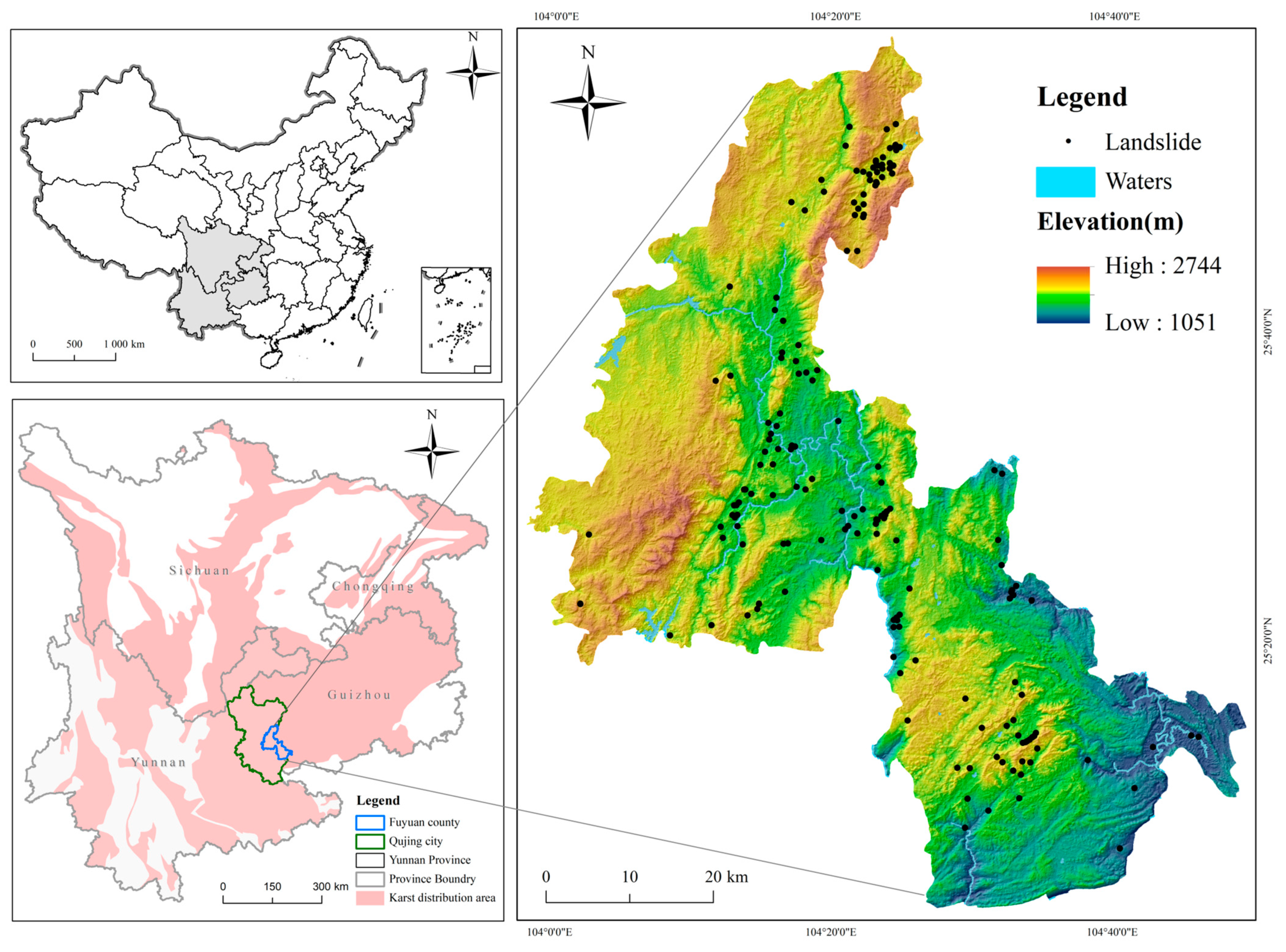
Figure 1. Geographical setting of the study area.
Water 16 02414 g001
Figure 2. Thematic map of some landslide impact factors: (a) surface deformation rate; (b) distance from faults; (c) distance from mining sites; (d) distance from roads; (e) distance from waters; (f) elevation; (g) lithology; (h) land surface temperature; (i) NDVI; (j) average annual rainfall; (k) soil bare rate; (l) surface cutting depth; (m) slope; (n) soil type; (o) aspect.
Water 16 02414 g002aWater 16 02414 g002b
Figure 3. Spatial and temporal baseline distributions.
Water 16 02414 g003
Figure 4. Distribution of surface deformation rate along the LOS direction in the study area.
Water 16 02414 g004
Figure 5. Technology roadmap.
Water 16 02414 g005
Figure 6. Flowchart of expanding sampling strategy.
Water 16 02414 g006
Figure 7. Distribution of deformation rate along the slope direction.
Water 16 02414 g007
Figure 8. ROC curves before sample expansion (a) and ROC curves after sample expansion (b).
Water 16 02414 g008
Figure 9. Landslide susceptibility mapping before sample expansion (a) and after sample expansion (b).
Water 16 02414 g009
Figure 10. SHAP summary plot of landslide conditioning factors after sample expansion.
Water 16 02414 g010
Figure 11. Importance ranking plot of landslide conditioning factors after sample expansion.
Water 16 02414 g011
Figure 12. One-factor partial dependence plots after sample expansion: (a) Distance from mining site; (b) NDVI; (c) surface deformation rate; (d) surface temperature. (The horizontal coordinates indicate the grading intervals for each condition factor, which correspond to the grading criteria in Table 3).
Water 16 02414 g012aWater 16 02414 g012b
Table 1. Data and sources.
Data NameData SourcesTypologyResolution
Historical landslide dataChinese Academy of Sciences, Center for Resource and Environmental Data and SciencesVector (spatial)-
DEMGeospatial data cloud platformRaster30 m
Landsat-8 dataGeospatial data cloud platformRaster30 m
Geological dataNational Geological Information Data Center (NGIDC)Vector (spatial)1:200,000
WatersChinese Academy of Sciences, Center for Resource and Environmental Data and SciencesVector (spatial)1:100,000
RoadsChinese Academy of Sciences, Center for Resource and Environmental Data and SciencesVector (spatial)1:100,000
Multi-year average rainfallChinese Academy of Sciences, Center for Resource and Environmental Data and Sciencesraster1000 m
Administrative subdivision (e.g., of provinces in counties)National Geographic Information Public Service PlatformVector (spatial)1:100,000
ProvenanceNational Address LibraryVector (spatial)-
Soil dataWorld Soil Database (HWSD)Raster1000 m
Sentinel-1 dataEarthData ASF Data SearchRaster30 m
Normalized
Difference
Vegetation
Index (NDVI)
National Science and Technology Resources Sharing Service PlatformRaster30 m
Table 2. Classification of landslide conditioning factors.
CategoriesConditioning FactorsClassification/UnitClassification Criteria
Topographic and geomorphologic factorsElevation (Ele)/m11(1) 1051–1427; (2) 1917–2012; (3) 1427–1580; (4) 2012–2099; (5) 1580–1711; (6) 1711–1818; (7) 1818–1917; (8) 2099–2189; (9) 2189–2299; (10) 2299–2439; (11) 2439–2744
Slope/°10(1) 0–5; (2) 5–10; (3) 10–15; (4) 15–20; (5) 20–25; (6) 25–30; (7) 30–35; (8) 35–40; (9) 40–50; (10) >50
Surface cutting depth (SCD)/m10(1) 0~31; (2) 31~47; (3) 47~61; (4) 61–75; (5) 75~90; (6) 90~107; (7) 107~125; (8) 125~148; (9) 148~180; (10) >180
Aspect10(1) plane (−1); (2) north (0–22.5); (3) northeast (22.5–67.5); (4) east (67.5–112.7); (5) southeast (112.5–157.5); (6) south (157.5–202.5); (7) southwest (202.5–247.5); (8) west (247.5–292.5); (9) northwest (292.5–337.5); (10) north (337.5–360)
Surface cover factorsSoil bare rate (SBR)7(1) <−80; (2) −80 to −55; (3) −55 to −36; (4) −36 to −24; (5) −24 to −16; (6) −16 to −11; (7) −11 to −1
Soil erosion modulus
(SEM)
9(1) <304; (2) 304–989; (3) 989–1749; (4) 1749–2661; (5) 2662–3802; (6) 3802–5171; (7) 5171–6920; (8) 6920–9581; (9) >9581
Land surface temperature
(LST)/°
9(1) <16; (2) 16–24; (3) 24–28; (4) 28–31; (5) 31–33; (6) 33–36; (7) 36–39; (8) 39–43; (9) 43–54
NDVI9(1) <0.20; (2) 0.20–0.33; (3) 0.33–0.43; (4) 0.43–0.52; (5) 0.52–0.59; (6) 0.59–0.66; (7) 0.66–0.74; (8) 0.74–0.83; (9) 0.83–0.99
Soil type (ST)18(1) Brown soil; (2) Lakes and waters; (3) Rock; (4) alluvial soil; (5) Yellow soil; (6) paddy soil; (7) Acidic purple clay; (8) Limestone; (9) Yellow-brown loamy soil; (10) Yellow-red soil; (11) black lime; (12) Yellow-brown soil; (13) mountainous red soil; (14) Red soil; (15) Red loamy soil; (16) Brick red soil; (17) calcium phosphate; (18) Dark brown soil
Hydrological factorsDistance from waters (DFW)/m9(1) <500; (2) 500–1000; (3) 1000–1500; (4) 1500–2000; (5) 2000–2500; (6) 2500–3000; (7) 3000–4000; (8) 4000–9000; (9) >9000
Average annual rainfall (AAR)/mm9(1) <1007; (2) 1007–1023; (3) 1023–1036; (4) 1036–1052; (5) 1052–1070; (6) 1070–1090; (7) 1090–1112; (8) 1112–1137; (9) >1137
Topographic wetness index (TWI)6(1) 2.08–4.88; (2) 4,88–6.33; (3) 6.33–8.13; (4) 8.13–10.48; (5) 10.48–13.95; (6) 13.95–30.62
Human activity factorsDistance from mining site (DFMS)/m10(1) <2300; (2) 2300–4141; (3) 4141–5889; (4) 5889–7545; (5) 7545–9201; (6) 9201–10,858; (7) 10,858–12,698; (8) 12,698–14,722; (9) 14,722–17,943; (10) >17,943
Distance from road (DFR)/m9(1) <428; (2) 428–909; (3) 909–1436; (4) 1436–2029; (5) 2029–1723; (6) 2723–3535; (7) 3535–4555; (8) 4555–6208; (9) >6208
Geological factorsLithology (Li)8(1) C1: lower Carboniferous; (2) C1P1: Carboniferous and Permian juxtaposition; (3) C2: upper Carboniferous; (4) D3C1: Devonian and Carboniferous juxtaposition; (5) P2: Upper Permian; (6) T1: Upper Triassic; (7) T2: middle Triassic; (8) T3:Lower Triassic
Distance from fault (DFF)/m9(1) <500; (2) 500–1000; (3) 1000–1500; (4) 1500–2000; (5) 2000–2500; (6) 2500–3000; (7) 3000–4000; (8) 4000–9000; (9) >9000
Surface deformation rate (SDR)/mm·a−19(1) <−78; (2) −78 to −50; (3) −50 to −35; (4) −35 to −23; (5) −23 to −12; (6) −12 to −1; (7) −1 to 9; (8) 9~26; (9) >26
Table 3. Basic parameter information of Sentinel-1A IW mode image data.
ParameterCorresponding Value
Acquisition of the satelliteSentinel-1A
OrbitAscending orbit
Resolution/m5 × 20
Polarization modeVV + VH
Revisit period/d12
Incidence angle/(°)38.99
Impact time February 2017–December 2017
Number of images/views34
Table 4. Confusion matrix before sample expansion (left) and confusion matrix plot after sample expansion (right).
Actual ValuePredicted ValueActual ValuePredicted Value
LandslideNon-LandslideLandslideNon-Landslide
Landslide435Landslide14912
Non-Landslide1541Non-Landslide23136
Table 5. Evaluation indexes of model accuracy.
SampleAccuracyPrecisionRecallF1-Score
Before Expanding Sample0.80770.89130.73210.8039
After Expanded Sample0.89060.91890.85530.8860
Table 6. Landslide susceptibility vs. distribution of the historical landslides.
SampleSusceptibility ClassProbability of Landslide OccurrenceGrid Number (pcs)Area Ratio (%)Number of Landslide Points (pcs)Density (pcs/km2)
Before Expanding SampleVery Low Susceptibility Zone<0.257977,06227.54530.003412
Low Susceptibility Zone0.257–0.392849,14423.938130.017011
Medium Susceptibility Zone0.392–0.521828,71623.362180.024134
High Susceptibility Zone0.521–0.662565,74915.949540.106054
Very High Susceptibility Zone>0.662326,6299.208850.289149
After Expanded SampleVery Low Susceptibility Zone<0.1231,530,46743.14510.000726
Low Susceptibility Zone0.123–0.2301,042,70829.394200.021312
Medium Susceptibility Zone0.230–0.418547,52015.435340.068998
High Susceptibility Zone0.418–0.648281,6147.938610.240676
Very High Susceptibility Zone>0.648144,9914.087570.436809
Disclaimer/Publisher’s Note: The statements, opinions and data contained in all publications are solely those of the individual author(s) and contributor(s) and not of MDPI and/or the editor(s). MDPI and/or the editor(s) disclaim responsibility for any injury to people or property resulting from any ideas, methods, instructions or products referred to in the content.