Article

Fine-Resolution Wetland Mapping in the Yellow River Basin Using Sentinel-1/2 Data via Zoning-Based Random Forest with Remote Sensing Feature Preferences

Key Laboratory of Remote Sensing and Digital Earth, Aerospace Information Research Institute, Chinese Academy of Sciences, Beijing 100101, China
*
Author to whom correspondence should be addressed.
Water 2024, 16(17), 2415; https://doi.org/10.3390/w16172415
Submission received: 13 July 2024 / Revised: 23 August 2024 / Accepted: 24 August 2024 / Published: 27 August 2024

Abstract

:
Accurate wetland classification in the Yellow River Basin (YRB) is crucial for China’s ecological security, sustainable development, and wetland resource management. This calls for more sustained research on regional variations and studies on remote sensing features, especially with temporal considerations. To address this and the optimization of feature extraction as well as ranking, Sentinel-1 and Sentinel-2 images were used. Additionally, to achieve more precise wetland classification, the YRB was subdivided into four regions for random forest classification. The results show that different remote sensing indices effectively distinguish various wetland types and that key percentiles play a significant role in distinguishing wetland types. The 10 m refined wetland classification map for 2020, with an overall accuracy of 85%, demonstrates that this framework can meet the needs of conventional large-scale wetland analysis and management. The total area of wetlands in the YRB in 2020 was 33,554.67 km2, mainly distributed in the upper reaches of the YRB (71%), with seasonal marshes being predominant. The total water area reached 8538.64 km2, primarily distributed in the upper reaches of the YRB (57.40%). This high-resolution wetland map offers crucial insights and tools for monitoring, protecting wetland resources, and shaping policies, advancing regional sustainable development goals.

1. Introduction

Wetlands are often referred to as the “kidneys of the earth” and “ecological supermarkets” due to their crucial role in maintaining ecosystem balance. The functions they provide could maintain water balance, mitigate the risks of floods and droughts, supply fiber and fish, regulate climate, and protect biodiversity [1,2]. The YRB, passing through nine provinces across north China, stands as one of the most crucial river systems in China and is considered an important barrier for national ecological security. And wetlands, with their unique ecological functions, are of great significance in the building of the national ecological security barrier. However, due to global climate changes and human interference, wetlands have experienced rapid declines in area in recent centuries [3]. From 1980 to 2015, the average annual decrease in marshes in the YRB was of 157.0 km2 [4]. Reductions in wetland area and changes in wetland types in the YRB have led to ecosystem degradation, higher risks of floods and droughts, and increased water pollution, threatening local farmland, cities, and people’s lives. Information on the area and distribution of wetlands is the basis for the protection and restoration of wetland ecosystems, and it is of great significance for ecological security and maintaining the balance of ecosystems in the YRB.
Currently, land use and land cover (LULC) products at the Chinese or global scale typically classify wetlands as a single type, lacking identification of wetland subtypes [5]. Additionally, classification algorithms employed at larger scales primarily aim to achieve an overall classification effect, potentially lacking detail in smaller regions. Consequently, the existing LULC maps cannot be directly utilized for the management and protection of wetlands within the YRB. In contrast, extensive research has been conducted focusing on high-altitude wetlands and coastal wetlands. For instance, Zhang et al. [6] compared the effectiveness of wetland information extraction in the Yellow River Delta under different remote sensing feature combinations, while Huo et al. [7] conducted a similar study in the Maqu wetland. Additionally, Hu et al. [8] classified and mapped typical salt marsh plant communities in the Yellow River Delta. More recently, Peng et al. [9] and Huang et al. [10] analyzed spatiotemporal changes in wetlands across the YRB utilizing Landsat images. However, these studies fall short, primarily due to the limited scope of wetland types examined and the inadequate resolution of the images employed.
Among numerous wetland classification studies, the most common approach is the utilization of Google Earth Engine (GEE) [11] due to its convenience in utilizing open remote sensing data and machine learning tools. For instance, GEE offers MODIS, Landsat, and Sentinel data, each with varying degrees of preprocessing, which are extensively utilized in wetland classification [12,13]. However, MODIS images, with a spatial resolution of 250 m, and Landsat images, with a spatial resolution of 30 m, may struggle to identify small-scale wetlands, resulting in the loss of critical local wetland information [14]. In contrast, Sentinel-1/2 images are increasingly being used for wetland classification due to their refined spatial resolution and dense temporal coverage [15,16]. Additionally, GEE facilitates the definition and application of diverse classification algorithms, including decision trees (DTs), support vector machines (SVMs), and random forests (RFs) [17,18,19,20], thereby enhancing the efficiency of wetland information retrieval. Random forests are insensitive to noise and overfitting, making them easier to implement and demonstrating higher classification accuracy in various wetland studies [21,22]. Currently, both pixel-based and object-based machine learning approaches have been proven effective in wetland landscape classification. Object-based image analysis (OBIA) supplements the limitations of individual pixels by offering features such as shape, texture, and background, crucial for wetland mapping. However, it is worth noting that many established pixel-based methods are often simpler, faster [23], and provide a clearer indication of each feature’s contribution to the classification process, compared to OBIA [24].
To a certain extent, the selection of wetland remote sensing features determines the outcomes of wetland classification, and choosing an excessive number of features can lead to redundancy, thus reducing classification accuracy. The Jeffries–Matusita (JM) distance [25] measures the spectral separability between class density functions, focusing specifically on the inherent distinguishability of features. Feature importance ranking in random forests [26] assesses each feature’s contribution to model performance. Together, they provide a comprehensive evaluation for selecting optimal wetland remote sensing features, enhancing classification accuracy, and reducing costs.
Furthermore, due to the environmental heterogeneity and temporal dynamics of wetlands, using single or mean composite images without temporal considerations may lead to misclassification in wetland mapping. Time series statistical indicators, such as percentile values for specific time spans, capture the magnitude of reflectance changes but do not explicitly capture time, potentially resulting in different phenological changes for the same land cover at different time series positions. Remote sensing images suffer from data loss due to cloud cover, acquisition frequency, and sensor issues, while time metrics demonstrate robustness. Zhang and Roy [27] used 20th, 50th, and 80th percentile composites from Landsat data for North American land cover mapping, reducing sensitivity to shadows, clouds, and pollution. Hansen et al. [28] generated US land cover products from Landsat data by extracting multiple percentile values, adapting to missing or cloudy pixels. Time metrics, as a statistical tool, demonstrate robustness and to some extent reflect phenological changes in land cover.
Based on the issues mentioned above, this study aims to (1) analyze wetland remote sensing features of Sentinel-1/2 for the YRB based on the GEE platform; (2) utilize the random forest classification model and empirical rules to produce fine wetland maps with a spatial resolution of 10 m; (3) analyze the spatial pattern of wetlands in the YRB. The fine wetland maps are expected to support the improvement in wetland ecological conservation and management mechanisms in the YRB.

2. Materials and Methods

2.1. Study Area

The Yellow River originates in Qinghai’s Bayankara Mountains, traversing 9 provinces before discharging into the Bohai Sea in Shandong. The YRB (30–42° N, 94–120° E) spans 7.95 × 10⁵ km2, or 8.3% of China’s land, serving as a vital security barrier and eco-economic corridor [29]. Its terrain slopes from west to east, with elevations varying from 0 to 6272 m [30], reflecting diverse ecosystems. The western plateau exceeds 4000 m, the central Loess Plateau is in the range of 1000–2000 m, and the alluvial plain dips below 100 m. The YRB’s continental climate, situated in a semi-arid to semi-humid transition zone [31], sees annual precipitation averaging 530–630 mm, mostly in summer. Maritime monsoons shape its ecosystem, transitioning from forests/grasslands in the southeast to grasslands/desert grasslands in the northwest [32]. Topographically, climatically, and vegetatively, the YRB is divided into upper, middle, and lower reaches.
Given the varying climates and geographies, the YRB is segmented into four regions (Figure 1b). Zone A, the upper reaches, boasts an arid climate, high altitude (3600 m), low annual temperature (0.5 °C), and abundant precipitation (>500 mm/yr), featuring wetlands like Shouqu and Zoige. Zone B, the middle reaches, exhibits a semi-arid monsoon climate, moderate altitude (1300 m), warmer temperature (8.4 °C avg.), and less rain (400 mm/yr), highlighted by the Inner Mongolia Linhe Wetland. Zones C and D, the lower reaches, share a maritime semi-humid climate, lower altitude (540 m), warmer avg. temperature (12.5 °C), and ample rainfall (>600 mm/yr). Zone D uniquely encompasses the Yellow River Delta’s coastal area, excluding artificial structures, due to its unique environment and remote sensing challenges posed by tidal flats.

2.2. Dataset

2.2.1. Remote Sensing Images

This study integrated 3004 Sentinel-1 SAR and 7953 Sentinel-2 MSI images (total 10,957) on GEE. Sentinel-1 images were pre-processed to remove noise and calibrated, while Sentinel-2 images were cloud-masked. In 2020, there were a larger number of available Sentinel-1 images in the upper and lower reaches of the YRB, with most areas having over 60 scenes, while in the middle and lower reaches, most areas were covered by 10–50 scenes of Sentinel-2 images (Figure 2). Time series data were reduced using GEE’s ee. Reducer. percentile to create 2020 composites, capturing 20th, 50th, and 80th percentiles. This condensed data size, include temporal information, and allowed for faster and more efficient image analysis. Time metrics can summarize multi-temporal spatial features, to some extent reflecting the trend in image data changes at different periods, including vegetation emergence, growth, and decline in various phenological stages, without being limited to specific years [33].

2.2.2. Sample Data

Referring to the definition of wetlands in the Ramsar Convention and field surveys conducted in the YRB, the wetlands were categorized as vegetation wetlands and water bodies (Table 1). Vegetation wetlands were further classified based on the vegetation coverage into floodplain wetlands (inland), tidal flats (coastal) and marshes (inland), and salt marshes (coastal) and swamps (inland). Marshes were further divided into seasonal marshes and permanent marshes based on their temporal dynamics. Additionally, although rice production has never been a dominant crop in the local food crops, rice cultivation has a long history in the YRB and belongs to the single-cropping rice cultivation area. Rice paddies are artificially managed and artificial marshes are regularly changed, which are of great significance for agricultural development in the YRB. This study classifies rice paddies as a separate category for analysis.
The wetland sample dataset was obtained through two steps: generating potential samples based on auxiliary datasets and corrections based on high-resolution images from Google Earth. This study used the publicly available wetland mapping product dataset from the Global Lakes and Wetlands Database [34] as a reference dataset to generate wetland sample points. Differentiation was conducted based on the definitions of seasonal and permanent marshes, combined with existing experiential rules. Specifically, based on all valid LSWI values throughout the year at the sample point, if the number of times LSWI > 0.4 exceeds LSWI < 0.3, the sample point is classified as a permanent marsh; otherwise, it is classified as a seasonal marsh. For rice paddies, reference was made to the dataset of rice planting areas in the Asian monsoon region from 2000 to 2021 published by the Beijing Normal University team [35], which exhibits good consistency with agricultural statistics data (R2 > 0.80). JRC Surface Water data [36] were used for water body sample data production.
The number of samples for each type is shown in Table 1. The spatial distribution of sample data is illustrated in Figure 1a. On the GEE platform, points were randomly selected on the wetland layer by directly calling or importing auxiliary datasets. The sample points were then exported in KML format and imported into Google Earth. A series of historical high-resolution images were viewed using the time slider to ensure that the sample points remained wetland samples throughout the year 2020. This approach enhances sample stability by detecting changes within each landscape year. Additionally, 5120 non-wetland samples were randomly selected through visual interpretation, resulting in a total of 10,224 sample data points generated. Finally, 70% of the sample data were allocated for the development of the wetland classification algorithm in the YRB, while the remaining 30% were reserved for classification accuracy verification.

2.2.3. Auxiliary Data

The Digital Elevation Model (DEM) with a spatial resolution of 30 m provided by the Shuttle Radar Topography Mission (SRTM) was used to generate terrain information such as elevation, slope, and aspect. Additionally, with the three datasets, including the ESA_Worldcover [37], CAS_Wetlands [38], and GWL_FCS30 wetland datasets [39], were compared with our research result. ESA WorldCover is a product developed by the European Space Agency (ESA), which provides a global land cover map for 2020 with a spatial resolution of 10 m based on Sentinel-1 and Sentinel-2 data. CAS_Wetlands offers data with a 30 m resolution produced by the Northeast Institute of Geography and Agroecology (NEIGAE) research team in 2015. The GWL_FCS30 which includes eight wetland sub-categories achieved an overall accuracy of 86.44% and was stored with a spatial resolution of 30 m in the GeoTIFF format.

2.3. Methods

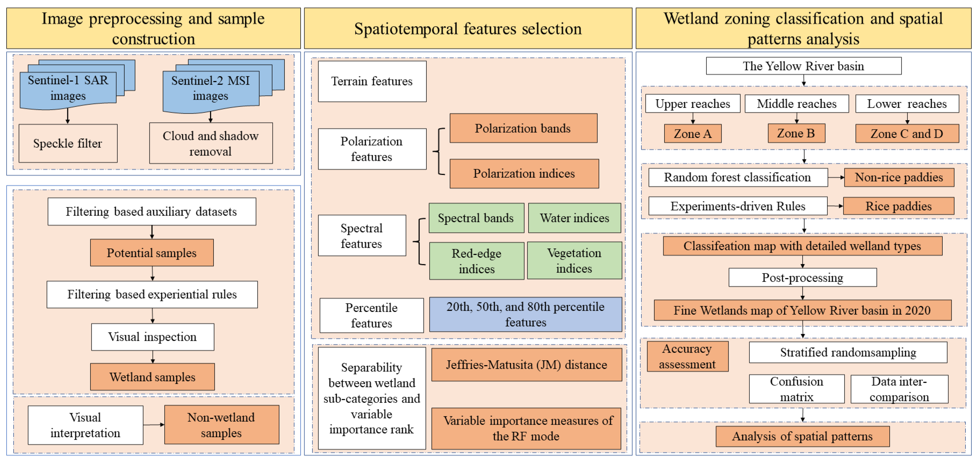
The workflow of wetland classification in this study can be outlined in three main steps (Figure 3). Firstly, this study analyzed the separability and importance of remote sensing classification features for various wetland types across the YRB, thus providing highly applicable and transferable insights into remote sensing feature application. Secondly, Sentinel-1/2 image data were employed to address the issue of local information loss resulting from the current use of spatial resolutions of 30 m and below for wetland classification in the YRB. Thirdly, a classification scheme tailored to the ecological differences in wetlands in distinct zones of the YRB was formulated, thus mitigating the risk of spatial distribution errors that could arise from generalized classification. Finally, the spatial patterns of wetlands in the YRB were analyzed.

2.3.1. Features Extraction

This study utilized a comprehensive set of remote sensing classification features (Table 2), including spectral features [7] (9 spectral bands and 16 spectral indices categorized into vegetation indices, water indices, and red-edge indices and polarization features (VV, VH, and derived metrics like SAR_Diff, SAR_Sum, VVrVH, and SAR_NDVI)). Additionally, terrain features (elevation, slope, and aspect) were computed based on the SRTM dataset. To effectively capture the seasonal characteristics of wetlands and non-wetlands, a multi-source feature time series stack utilizing both Sentinel-1/2 images was constructed. Based on the time series of spectral and polarization features, percentile features were synthesized. Specifically, within GEE, the 20th, 50th, and 80th percentile features were computed. This involved first calculating the spectral index histograms for each pixel based on the 2020 time series data, and then extracting the percentile features at the specified values (i.e., 20%, 50%, 80%) for each pixel [27]. As a result, this study generated a phenology-based feature set comprising a total of 96 feature layers, reflecting the diverse seasonal patterns captured from the multi-source data.

2.3.2. The Method of Analyzing Separability between Wetland Sub-Categories

In this study, the separability between wetland categories was qualitatively determined using box plots, and the Jeffries–Matusita (JM) distance was quantitatively used to determine the separability between wetland categories. The JM distance is based on the assumption of normal data distribution and describes the separability of feature subsets between different categories, without requiring a specific distribution form for the input data, thus being widely used in the fields of pattern recognition and feature selection [25].
The larger the distance, the smaller the similarity between categories. The JM separability criterion between two target land classes w i and w j in the training sample set C ( i , j = 1,2 , , C , i j ) is defined as follows:
J i j = 2 ( 1 e d i j )
where d i j is the Bhattacharyya distance between two target land classes w i and w j , defined as follows:
d i j = I n P x / w i P ( x / w j ) d x
In the above equation, P x / w i and P ( x / w j ) are the conditional probability density functions of the random variable x for land classes w i and w j , respectively, typically assumed to be multivariate normal distributions. The expression for Bhattacharyya distance is as follows:
d i j = 1 8 m j m i T i + j 2 1 m j m i + 1 2 I n i + j 2 i j
where m i and m j represent the means; i and j represent the covariance matrices of w i and w j , respectively, and the superscript T denotes the transpose of the matrix. The JM distance ranges from 0 to 2, and it is generally considered that a JM distance greater than 1.8 indicates good separability between land cover types, between 1.4 and 1.8 indicates moderate separability, and smaller than 1.4 indicates high similarity in feature variables between land cover categories, making them difficult to distinguish.

2.3.3. Importance of Remote Sensing Classification Features

All classification features greater than 1.4 were used to train the RF model. However, not every feature equally contributed to classification accuracy. To reduce data redundancy and improve algorithm efficiency, feature dimensionality reduction was implemented on the GEE based on random forest to rank the importance of remote sensing classification features. Initially, the “ee.Classifier.explain” function was used to output the variable importance measures computed by the RF model. Then, the measurement results were sorted in descending order, and the first n features were sequentially inputted into the RF model for training and classification, thereby obtaining the overall accuracy for each combination. Finally, the combination with the highest overall accuracy and the least number of features was determined for the wetland classification algorithm in the YRB.

2.3.4. Wetland Classification in the YRB

Based on phenological characteristics, this study implemented pixel-based random forest classification using the GEE platform. Firstly, independent RF classifiers were trained for each ecological region of the YRB. Considering accuracy and computational efficiency, the number of trees determining the forest size in RF parameters was set to 100. The remote sensing classification features involved in classification were determined by variable importance measures and sorting results. Finally, by integrating the results of all ecological regions, an initial wetland map was generated, including non-wetland, water bodies, swamps, seasonal marshes, permanent marshes, rice paddies, floodplain wetlands, and tidal flats.
Rice paddies belong to artificial wetlands and are subject to regular irrigation, making them a relatively difficult type to distinguish. Rice cultivation in the YRB is of single-season type, making it easily confused with cultivated land [35]. Therefore, within the independently classified rice paddy layer, a reclassification was conducted to remove misclassified cropland. After numerous experiments, it was found that the combination of NDWI and RVI exhibited good discriminability between rice paddies and cropland. The classified rice paddy layer was subjected to thresholding, where parts meeting the following conditions were identified as rice paddies, while the rest were classified as non-wetlands: NDWIP20 < −0.35 and RVIaverage > 2.
The Mapping Composite tool in the Spatial Analyst extension module of ArcGIS 10.2 software was utilized in the post-processing of wetland classification results. To eliminate the impact of the “salt and pepper” phenomenon on spatial pattern analysis, isolated pixels or noise were first removed from the classification output using the Majority Filter tool. Subsequently, the Boundary Clean tool was employed to smooth irregular class boundaries and perform clustering of classes. Finally, the Region Group, Set Null, and Half Byte tools were used sequentially to reclassify smaller isolated pixel areas into the nearest class.

2.3.5. Accuracy Assessment of YRB Wetland Classification Results

Accuracy was assessed using a confusion matrix, calculating overall accuracy (OA), kappa coefficient, user accuracy (UA), and producer accuracy (PA) [40]. OA measures overall algorithm efficiency, kappa assesses agreement with actual data, UA reflects the accuracy of the classified pixels, and PA assesses the correct identification of reference samples. The YRB results were also compared with other wetland datasets to ensure reliability.

3. Results

3.1. Selection of Remote Sensing Features for Wetlands

3.1.1. Separability of Wetland Sub-Categories Characterized by Different Features

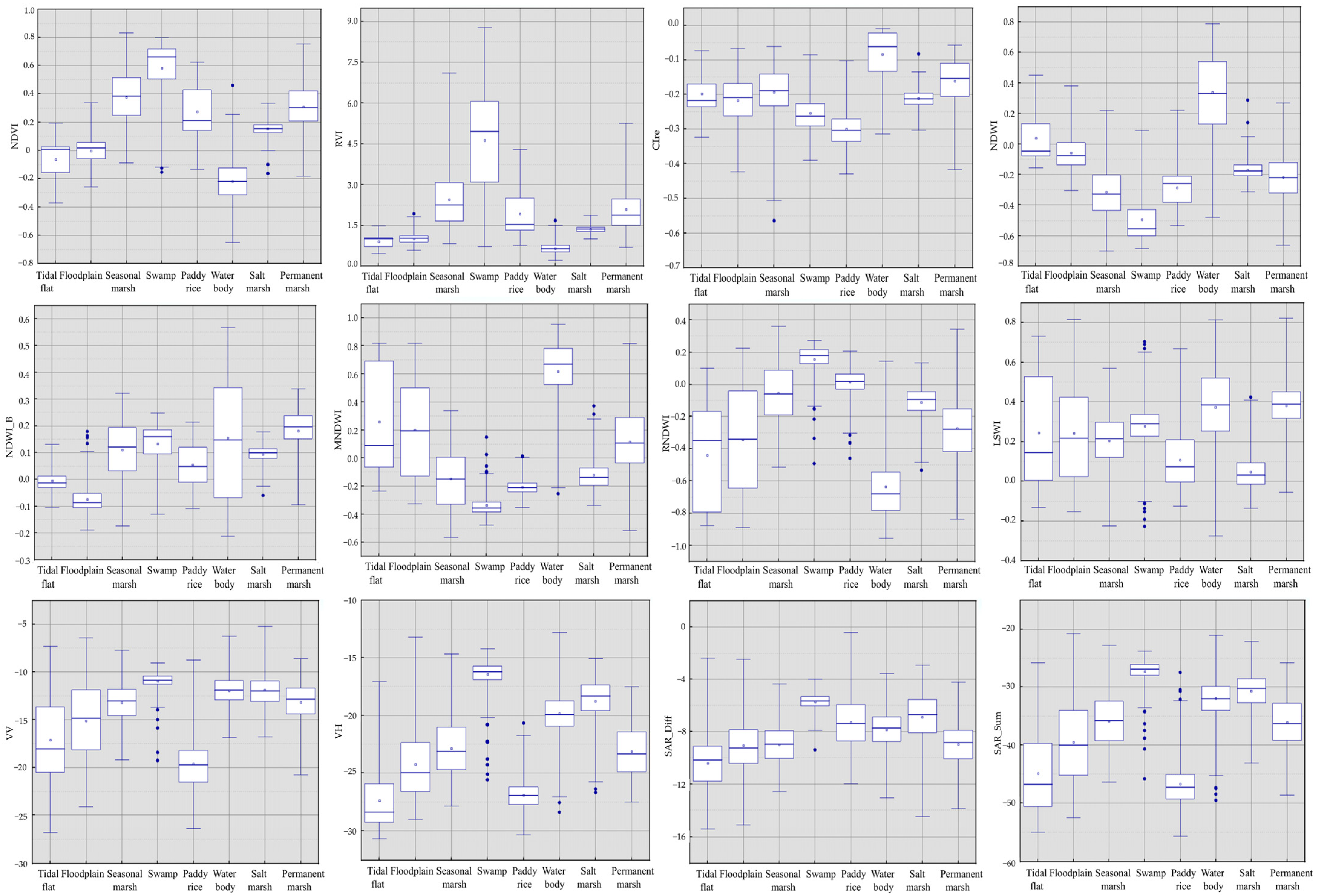
To test the discriminative ability of different remote sensing index features, the median, mean, upper, and lower quartiles, and 1.5 times the interquartile range (IQR) were conducted for all wetland categories of remote sensing index features (Figure 4). Additionally, individual outliers of remote sensing index features were also presented by blue dots in Figure 4. From the perspective of wetland types, swamps and water bodies can be well distinguished from other wetland types. Nevertheless, distinguishing among tidal flats, floodplains, seasonal marshes, rice paddies, salt marshes, and permanent marshes poses challenges due to their similar vegetation cover and hydrological environments.
In terms of vegetation indices, NDVI and RVI can better distinguish salt marshes from permanent marshes and seasonal marshes. The red-edge index exhibited similar separability as the vegetation indices, but CIre showed better separability between seasonal marshes and rice paddies. Regarding water body indices, the LSWI of salt marshes was lower than that of seasonal marshes, permanent marshes, and rice paddies; the RNDWI of permanent marshes was lower than that of seasonal marshes, rice paddies, and salt marshes, which can distinguish wetland types that were difficult to distinguish by vegetation indices. NDWI_B had a certain ability to distinguish tidal flats and floodplains. MNDWI, NDWI, and RNDWI can also better distinguish swamps from seasonal marshes and rice paddies. In the realm of polarization features, VH, SAR_Sum, and SAR_Diff exhibited potential in distinguishing tidal flats and floodplains. Notably, VH effectively discriminated rice paddies from seasonal and permanent marshes, while also demonstrating a certain degree of effectiveness in distinguishing rice paddies from salt marshes. However, as observed from box plots, VVrVH and SAR_NDVI did not exhibit outstanding performance in distinguishing between various wetland types.

3.1.2. Jeffries–Matusita (JM) Distances between Pairs of Wetland Sub-Categories

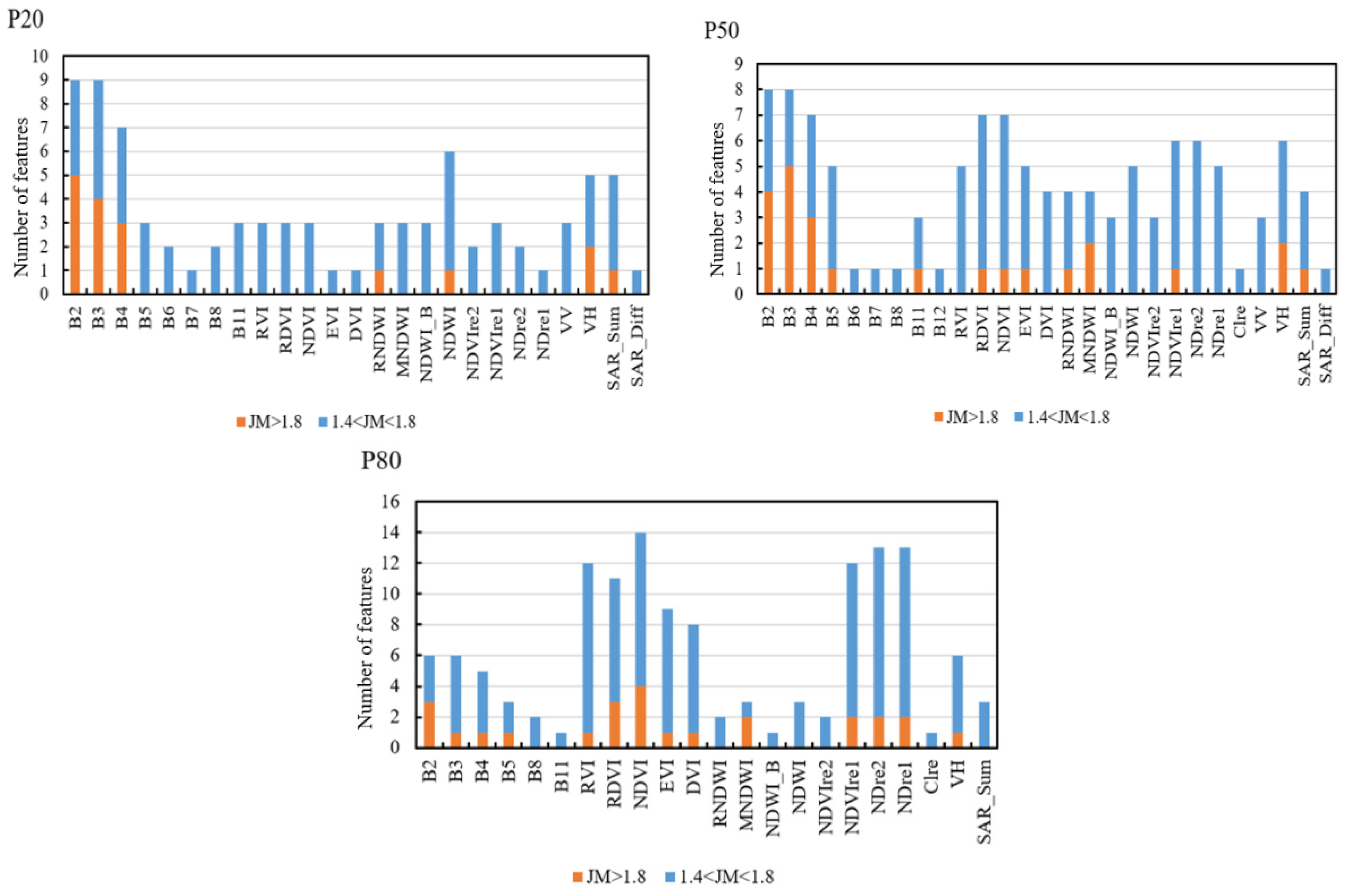
Calculating the JM distance between feature variables of different wetland types serves as an effective method to evaluate their separability. To this end, this study computed the JM distances at the 20th (P20), 50th (P50), and 80th (P80) percentiles for a comprehensive set of feature variables, including spectral features (B2, B3, B4, B5, B6, B7, B8, B11, B12), vegetation indices (NDVI, DVI, RVI, RNDVI, EVI), water indices (NDWI_B, NDWI, MNDWI, RDWI, LSWI), red-edge indices (NDVIre1, NDVIre2, NDVIre3, NDre1, NDre2, CIre), and polarization features (VV, VH, SAR_Sum, SAR_NDVI, SAR_Diff, VVrVH). By analyzing these JM distances, this study aimed to provide insights into the discriminability of different wetland types (Figure 5).
For the 20th (P20) and 50th (P50) percentiles, the spectral bands B2, B3, and B4 frequently occurred within the JM distance ranges of 1.4–1.8 and greater than 1.8, suggesting that the red, green, and blue light bands were major contributors to wetland classification at these percentiles. In P50 and P80, vegetation indices such as RVI, RNDVI, and NDVI dominated the range of 1.4–1.8, emphasizing their significant role in wetland discrimination at the 50th and 80th percentiles.
In P80, specifically, there was a notable increase in the occurrence of red-edge indices within both the 1.4 to 1.8 and greater than 1.8 JM distance ranges. Notably, NDVIre1, NDre1, and NDre2 were more prevalent in P80 compared to P20 or P50, indicating a heightened contribution of red-edge indices to wetland classification at the 80th percentile, with the lowest contribution observed in P20.
Water indices consistently contributed across P20, P50, and P80, with NDWI emerging as the most frequent and influential among them. Among the polarization features, VH was the most prevalent within the JM distance ranges of interest, closely followed by SAR_Sum, indicating that VH and SAR_Sum were the primary contributors to wetland classification among the polarization characteristics.
In the analysis of JM distances between diverse feature variables of wetland types, 20 groups were identified with JM > 1.4, 8 of which exceeded JM > 1.8 (Table A1). These results indicate that, using specific water body indices and vegetation indices, combinations such as water bodies and swamps, water bodies and rice paddies, and others, could be easily distinguished.
Table A2 further details wetland type combinations and associated feature variables within the range of 1.4 < JM < 1.8, excluding those that had already met the criteria of JM > 1.8. Notably, under the JM distance framework, the separability between permanent marshes and swamps was only evident in the 20th percentile water index LSWI, along with the polarization features VH and SAR_Sum. Similarly, the distinction between floodplain wetlands and salt marshes was solely captured by the 20th percentile NDWI_B. Conversely, the separability between rice paddies and floodplain wetlands emerged only in the 80th percentile, marked by vegetation indices and red-edge indices.
These findings underscored the importance of considering feature variables in both the 20th and 80th percentiles when classifying wetlands. Interestingly, among all examined feature variables, NDVIrel3, VVrVH, and SAR_NDVI did not make an appearance in the list where JM exceeded 1.4.

3.1.3. Variable Importance Measures of the RF Model and the Overall Accuracy of Different Feature Combinations

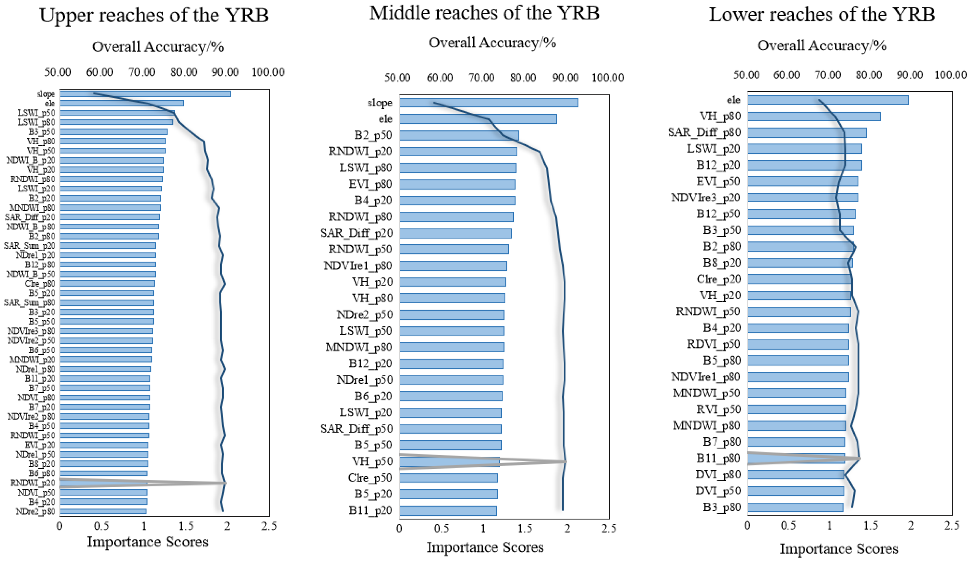
The analysis of importance scores for different feature variables revealed that elevation and slope were highly significant terrain features, whereas aspect scores were relatively low. Figure 6 illustrates the relationship between various feature combinations and classification accuracy. As the number of feature variables increased, classification accuracy initially surged, followed by a plateauing trend, particularly after the inclusion of the first five variables. Specifically, in the upper reaches of the YRB in 2020, accuracy rose dramatically from 58.26% to 80.95%, primarily attributed to the high importance scores, low redundancy, and minimal correlation among the initial feature variables. This significantly enhanced the classifier’s performance. Subsequently, while accuracy continued to improve gradually, the rate of change decelerated, stabilizing above 84.95% and peaking at 89.58% with 42 feature variables. However, a slight decline was observed, with accuracy dropping to 88.58% when the number of variables reached 90. Therefore, the first 42 features were chosen as the optimal set for classification in the upper reaches of the YRB in 2020. Similarly, for the middle and lower reaches, the top 24 and 38 features, respectively, based on their importance scores, were selected for final classification.

3.2. Accuracy Assessment of the YRB Wetland Classification Results

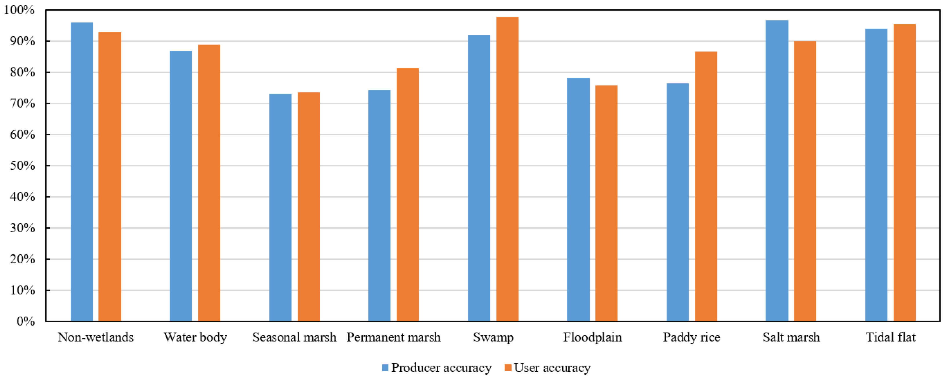
Visual verification indicated that the classification map based on the RF classifier, incorporating phenological, spectral, polarimetric, and terrain features, reliably depicts the distribution of wetlands in the YRB and has been shown to align closely with high-resolution imagery. Confusion matrix analysis based on 3068 validation samples indicated an overall classification accuracy of 85% and a kappa coefficient of 0.75 for the generated 2020 wetland map of the YRB (Figure 7), demonstrating high consistency with the validation samples. Mapping accuracy and user accuracy for salt marshes, tidal flats, and swamps exceeded 90%, as these wetland types were concentrated in the YRB. Mapping accuracy and user accuracy for water bodies were not less than 85%. Seasonal marshes, permanent marshes, floodplain wetlands, and rice paddies had mapping accuracy and user accuracy ranging from 70% to 80%.
It is noteworthy that swamps, salt marshes, tidal flats, and water bodies exhibited high accuracy and were easily distinguishable, whereas seasonal marshes, permanent marshes, and rice paddies had high spectral similarity, making them more difficult to distinguish. This was because these categories may share similar vegetation patterns and spectral reflectance, such as wet soils, dense vegetation, and some emergent vegetation, posing challenges to their classification. Overall, the classification results demonstrate that advanced classification techniques can improve the accuracy of wetland classification. The confusion matrices for each region of the YRB indicated that the overall accuracy of wetland classification results in each region exceeds 84%. Zone A had the highest accuracy (OA: 91.97%), followed by Zone B (OA: 91.22%), while the accuracies of Zone C (OA: 85.77%) and Zone D (OA: 84%) were slightly lower.

3.3. Spatial Pattern of Different Wetland Sub-Categories in the YRB

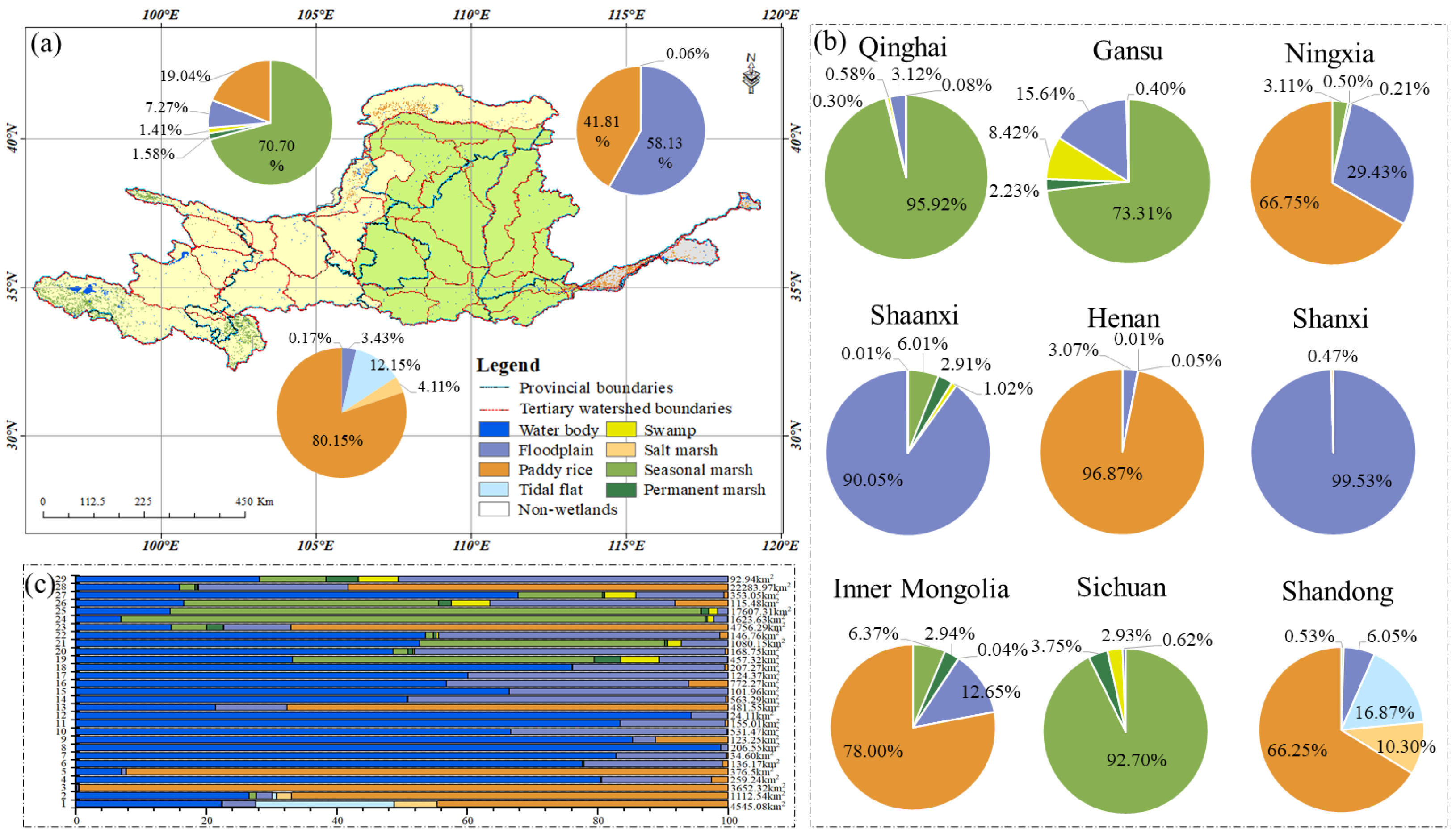
The wetlands in the YRB are widely distributed, covering a total area of 33,554.67 km2 in 2020 (Figure 8). Seasonal marshes were the dominant wetland type in the basin, accounting for 50.15% of the total wetland area. Rice paddies were prevalent in Zones A, B, and C of the YRB, occupying 34.00% of the total wetland area. Floodplain wetlands contributed 9.05% to the total wetland area. Tidal flats, permanent marshes, swamps, and salt marshes collectively comprised 6% of the total wetland area, with individual percentages of 2.89%, 1.12%, 1.01%, and 0.98%, respectively. The total water area within the YRB was 8538.64 km2, with the upper, middle, and lower reaches accounting for 57.40%, 27.11%, and 15.47% of this total area, respectively.
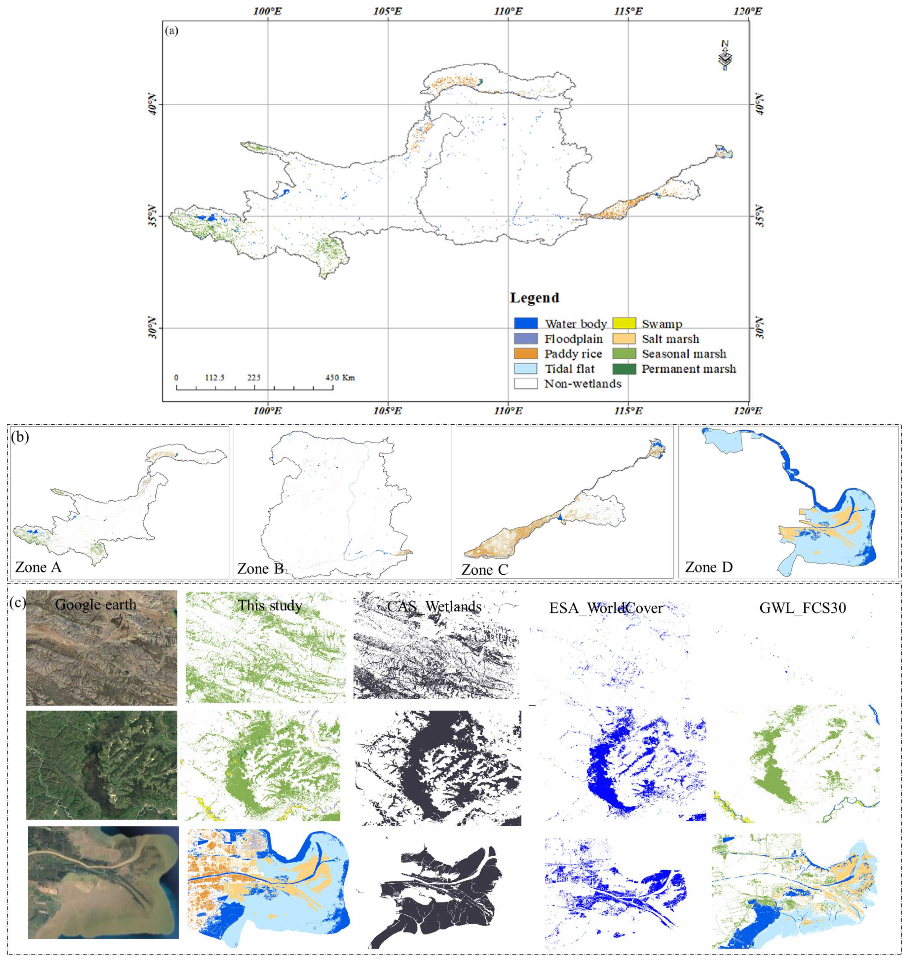
In 2020, the majority of wetlands in the YRB were concentrated in Zone A of the upper reaches, where seasonal marshes were particularly abundant. In contrast to Zone A in the upper reaches, wetlands in Zone B of the middle reaches were more dispersed, primarily concentrated in the northern part (Figure 9a,b). Tidal flats and salt marshes were predominantly distributed at the mouth of the Yellow River, specifically in Zones C and D of the lower reaches.
The total area of wetlands in Zone A of the upper reaches of the YRB was 23,784.08 km2 (Figure 8a), covering a relatively extensive region and comprising 71% of the total wetland area within the YRB. Seasonal marshes were the most widely distributed and predominant wetland type in this region, accounting for 70.70% of the total wetland area in the upper reaches. Rice paddies and floodplain wetlands followed, occupying 19.04% and 7.27% of the total wetland area, respectively. Swamps and permanent marshes had the smallest shares, together accounting for just 3.00% of the total wetland area in the upper reaches.
In Zone B of the middle reaches of the YRB, the total wetland area was 1782.28 km2 (Figure 8a), representing only 5.3% of the total wetland area in the entire basin. In contrast to the upper reaches, wetlands in Zone B were more concentrated in the northern part. Floodplain wetlands and rice paddies dominated, comprising 58.13% and 41.81% of the total wetland area in the middle reaches, respectively.
The lower reaches of the YRB, encompassing Zones C and D, exhibited a diverse range of wetland types with a total area of 7988.31 km2 (Figure 8a), contributing 23.80% to the total wetland area within the YRB. Rice paddies were the most prevalent wetland type in this region, covering 80.15% of the total wetland area in the lower reaches. Tidal flats, salt marshes, floodplain wetlands, and seasonal marshes, on the other hand, accounted for 12.15%, 4.11%, 3.43%, and 0.17% of the total wetland area in the lower reaches, respectively.
The YRB spans across nine provinces, each characterized by distinct predominant wetland types (Figure 8b). In Gansu, Sichuan, and Qinghai, seasonal marshes dominated, comprising 73.31%, 92.70%, and 95.92% of their respective provincial wetland areas. Conversely, rice paddies were prevalent in Shandong, Ningxia, and Inner Mongolia, accounting for 66.25%, 66.75%, and 78.00% of their wetland areas. Floodplain wetlands formed the majority in Shaanxi and Shanxi, occupying 90.05% and 99.53% of their respective wetland areas. Notably, Qinghai boasted the largest water area within the YRB, accounting for over half of the total at approximately 52.66%. Shandong followed closely behind, contributing 15.89% to the overall water area. In contrast, the combined water area of Shanxi and Shaanxi comprised less than 1% of the total water area in the YRB.
To facilitate a clearer view of the proportion of wetlands in each of the three-level sub-basins of the YRB, percentage bar charts were plotted (Figure 8c). There is a total of 29 third-level sub-basins in the YRB, which were divided into smaller blocks, revealing that each sub-basin contains water bodies, with almost all water bodies distributed from Sanmenxia to Xiaolangdi. Seasonal marshes were the main wetland type in the region above Xiangtang along the Datong River. Rice paddies were the main wetland type in the Jinhe River Tianran Wenyanqu Basin. Except for a few sub-basins, namely the Qindan River, Yiluo River, Sanmenxia to Xiaolangdi, and Longmen to Sanmenxia main stream, which were concentrated in the middle reaches and only comprised at most three wetland types, other basins consisted of multiple types.

4. Discussion

4.1. Intercomparison between Wetlands in This Study and Existing Products

To further validate the accuracy of the wetland maps in this study, comparisons were made with the widely recognized CAS_Wetlands wetland dataset, the ESA Global Land Cover dataset (wetlands layer), and the GWL_FCS30 wetland dataset with three typical locations in the YRB selected for comparative analysis (Figure 9c). The CAS_Wetlands wetland dataset provided detailed classification of wetlands in China, including swamps, marshes, lakes, rivers, coastal marshes, and tidal flats, but excludes floodplain wetlands and rice paddies. The latest publicly available product extended to 2015 and included only marsh wetlands, with a resolution of 30 m. The ESA Global Land Cover dataset contained wetlands and permanent water bodies, with a publicly available product for 2020 at a resolution of 10 m. The GWL_FCS30 dataset included five inland wetland sub-categories (permanent water, swamp, marsh, flooded flat, and saline) and coastal tidal wetland sub-categories (mangrove, salt marsh, and tidal flats), with a resolution of 30 m.
According to Qiu et al. [4], utilizing CAS_Wetlands for the entire YRB, the marsh area in 2015 was identified as 17,534.2 km2, while the combined area of lakes, rivers, and other water bodies totaled 9393.6 km2 as the total water area. In contrast, this study found the combined area of seasonal and permanent marshes to be 17,204.86 km2, differing by 329.34 km2 from CAS_Wetlands. Furthermore, the water area calculated in this study deviated by 854.96 km2 from the corresponding area in CAS_Wetlands. Notably, the CAS_Wetlands reference data indicated significantly smaller areas for tidal flats (13.1 km2) and salt marshes (123.6 km2) compared to the findings of this study.
Upon examining the study area’s scope map presented in the work of Qiu et al. [4], it became evident that the downstream estuary region of the YRB was narrower in scope than the one defined in this study. To ensure a comprehensive overview of tidal flats and salt marshes distributions, this study redefined the estuary’s outer boundary prior to classification, based on high-resolution images from Google Earth in 2020 (Figure 9b, Zone D). This redefinition likely accounted for the substantial disparity in salt marsh and tidal flat areas.
It is worth noting that the CAS_Wetlands reference data excluded rice paddies, resulting in a total YRB wetland area of 27,374.2 km2. When rice paddies were excluded from this study’s calculations, the total wetland area amounted to 30,417.36 km2, indicating that the CAS_Wetlands data underestimated the total wetland area compared to this study. This discrepancy can be attributed to the lower resolution of the CAS_Wetlands reference data, which may have overlooked smaller wetland patches. Moreover, this study incorporated floodplain wetlands that were not categorized in the CAS_Wetlands dataset, contributing to the larger total wetland area reported.
The wetland categories in this study were more detailed than those in the three datasets, and the spatial details were richer. Illustrations of three typical wetlands (Figure 9c) demonstrate these advantages. The wetland dataset in this study had higher spatial consistency with the CAS_Wetlands marsh dataset, but there were slight differences, especially in the downstream Yellow River Delta estuary area due to landscape changes from 2015 to 2020. In the same estuary area, this study’s spatial distribution was almost identical to the ESA and GWL_FCS30 datasets. However, in the western area of Zhaling Lake upstream, ESA and GWL_FCS30 identified fewer wetlands than this study and CAS_Wetlands. In the southern region of Maqu County, this study’s wetland distribution was more consistent with CAS_Wetlands and GWL_FCS30, while ESA and GWL_FCS30 showed significantly smaller ranges. The ESA product, being land cover data at a global scale, did not consider multiple wetland types, leading to a smaller wetland area compared to this study. The GWL_FCS30 wetland dataset included various wetland subcategories but did not distinguish seasonal marshes or consider rice paddies, and it failed to differentiate between coastal and inland areas, causing some marshes to be incorrectly categorized as salt marshes. This highlighted the importance of regional differentiation in wetland classification within the YRB. Like ESA, GWL_FCS30 operated on a global scale, resulting in a smaller wetland area compared to this study.

4.2. Limitations and Future Improvements

This study successfully generated high-precision maps of eight wetland types in the YRB. However, there are uncertainties and limitations. Firstly, this study did not further refine water bodies into categories such as aquaculture ponds, rivers, lakes, or reservoirs, which have certain practical value. For example, the extent of aquaculture ponds can be used to monitor the intensity of coastal zone development and support decisions regarding coastal wetland conservation and restoration. Secondly, the rules for distinguishing different topographic or geomorphic conditions in rice paddies were not differentiated. The uncertainty remains in the selection of remote sensing index features and thresholds for distinguishing rice paddy types. Due to the spectral similarity between rice paddies and croplands, even after rule-based screening, confusion still exists.
In future research, for wetland types exhibiting distinctive shape features, incorporating shape features into the classification process, along with manual correction and post-processing steps, can help refine and correct potential classification errors. Additionally, to broaden the applicability of this study, it is crucial to apply the wetland classification algorithm proposed herein to the long-term classification and dynamic monitoring of wetlands within the YRB. This will enable the revelation of the spatiotemporal evolution of specific wetland types, thereby providing invaluable insights and data to inform wetland resource conservation efforts and policy decision-making processes. Furthermore, exploring the utilization of alternative remote datasets (e.g., GF-series datasets) that could benefit similar studies, as well as examining other techniques beyond random forest (e.g., deep learning methods) that could be applied to enhance classification accuracy and robustness, would significantly enrich the research landscape and contribute to the advancement of wetland monitoring and management.

5. Conclusions

Based on the GEE platform and 2020 Sentinel-1/2 images, this study developed a refined wetland mapping framework for the YRB. The framework combined regional division, remote sensing feature selection, and the random forest algorithm, yielding a 10 m resolution wetland map with 85% OA and 0.75 kappa. Key features include spectral, vegetation, water body, red-edge indices, polarization, and topographic data. Temporal features via percentile composition algorithms also played a crucial role. The framework demonstrated its applicability in large-scale wetland analysis and management, highlighting the importance of integrating multi-source remote sensing data and temporal analysis for accurate wetland mapping. In 2020, the YRB’s 33,554.67 km2 wetland area was dominated by seasonal marshes in the upper reaches. The various wetland types varied in proportion, with a total water area of 8538.64 km2 distributed across the basin. The detailed wetland maps facilitate timely decisions for conservation and management in the YRB.

Author Contributions

Conceptualization, Methodology, Formal Analysis, and Writing—Original Draft Preparation, X.H.; Writing—Review and Editing, Supervision, Z.N. All authors have read and agreed to the published version of the manuscript.

Funding

This research was funded by Science & Technology Fundamental Resources Investigation Program, grant number 2022FY100302.

Data Availability Statement

The data presented in this study are available upon request from the corresponding author.

Conflicts of Interest

The authors declare no conflicts of interest.

Appendix A

Table A1. Characteristic variables for different wetland combinations with JM > 1.8.
Wetland TypesJM > 1.8Wetland TypesJM > 1.8Wetland TypesJM > 1.8
Paddy rice and water bodyMNDWI_P50Water body and swampNDVIre1_P80 B5_P50
RNDWI_P50NDre2_P80VH_P50
B11_P50EVI_P80B2_P20
RNDWI_P20MNDWI_P80B3_P20
MNDWI_P80NDre1_P80B4_P20
RDVI_P80DVI_P80VH_P20
Paddy rice and swampB2_P50VH_P80NDWI_P20
B3_P50Seasonal marsh and tidal flatB2_P50B2_P80
B2_P20B3_P50Swamp and tidal flatB3_P80
B2_P80B4_P50B4_P80
Water body and seasonal marshNDVI_P80B2_P20NDVI_P80
Water body and swampVH_P50B3_P20NDre1_P80
SAR_Sum_P50B4_P20NDVIre1_P80
NDVI_P50NDVI_P80B5_P80
RDVI_P50Swamp and floodplainB4_P50RDVI_P80
NDVIre1_P50B3_P50NDre2_P80
MNDWI_P50B3_P20RVI_P80
EVI_P50B4_P20Swamp and salt marshB2_P50
SAR_Sum_P20B2_P20B3_P50
VH_P20Swamp and tidal flatB2_P50B2_P20
NDVI_P80B3_P50B3_P20
RDVI_P80B4_P50B2_P80
Table A2. Characteristic variables for different wetland combinations with 1.4 < JM < 1.8.
Wetland Types1.4 < JM < 1.8Wetland Types1.4 < JM < 1.8Wetland Types1.4 < JM < 1.8
Paddy rice and seasonal marshB2_P50Water body and salt marshEVI_P50Seasonal marsh and floodplainB4_P50
Paddy rice and floodplainNDVI_P80NDVI_P50B3_P50
NDre2_P80DVI_P50B4_P20
NDre1_P80RNDWI_P50B3_P20
EVI_P80NDVIre2_P50NDVI_P80
RDVI_P80VV_P50NDre2_P80
NDVIre1_P80NDWI_P50NDre1_P80
DVI_P80NDre2_P50NDVIre1_P80
Paddy rice and tidal flatVH_P50SAR_Sum_P20Permanent marsh and floodplainNDWI_B_P20
NDWI_P20RVI_P20B4_P20
B2_P20B11_P20NDWI_B_P50
B3_P20NDVIre1_P20Permanent marsh & SwampVH_P20
NDVI_P80VV_P20LSWI_P20
RDVI_P80NDVI_P20SAR_Sum_P20
NDre1_P80RDVI_P20Floodplain & Salt marshNDWI_B_P20
DVI_P80MNDWI_P20Tidal flat and salt marshVH_P50
EVI_P80VH_P20B3_P50
NDre2_P80RNDWI_P20B3_P20
NDVIre1_P80NDVIre2_P20VH_P20
RVI_P80NDre2_P20B2_P20
VH_P80NDre1_P20VH_P80
B8_P80B8_P20B3_P80
Water body and permanent marshNDVI_P50MNDWI_P80NDre1_P80
NDVI_P80VH_P80NDre2_P80
NDre2_P80EVI_P80NDVI_P80
RDVI_P80RDVI_P80NDVIre1_P80
NDVIre1_P80NDre2_P80RVI_P80
NDre1_P80NDVIre1_P80EVI_P80
RVI_P80NDVI_P80RDVI_P80
Water body and salt marshMNDWI_P50DVI_P80Permanent marsh & Salt marshB4_P50
VH_P50NDWI_P80B2_P50
SAR_Sum_P50SAR_Sum_P80B3_P50
B11_P50NDre1_P80NDWI_B_P50
RDVI_P50RVI_P80B4_P20
RVI_P50Seasonal marsh and salt marshB2_P50B3_P20
NDVIre1_P50B2_P20B2_P20

References

  1. Niu, Z.; Zhang, H.; Wang, X.; Yao, W.; Zhou, D.; Zhao, K.; Zhao, H.; Li, N.; Huang, H.; Li, C.; et al. Mapping Wetland Changes in China between 1978 and 2008. Chin. Sci. Bull. 2012, 57, 2813–2823. [Google Scholar] [CrossRef]
  2. Xu, P.; Herold, M.; Tsendbazar, N.-E.; Clevers, J.G.P.W. Towards a Comprehensive and Consistent Global Aquatic Land Cover Characterization Framework Addressing Multiple User Needs. Remote Sens. Environ. 2020, 250, 112034. [Google Scholar] [CrossRef]
  3. Hu, S.; Niu, Z.; Chen, Y.; Li, L.; Zhang, H. Global Wetlands: Potential Distribution, Wetland Loss, and Status. Sci. Total Environ. 2017, 586, 319–327. [Google Scholar] [CrossRef]
  4. Qiu, Z.; Mao, D.; Xiang, H.; Du, B.; Wang, Z. Patterns and Changes of Wetlands in the Yellow River Basin for 5 Periods. Wetl. Sci. 2021, 19, 518–526. [Google Scholar] [CrossRef]
  5. Li, Z.; He, W.; Cheng, M.; Hu, J.; Yang, G.; Zhang, H. SinoLC-1: The First 1-meter Resolution National-Scale Land-Cover Map of China Created with a Deep Learning Framework and Open-Access Data. Earth Syst. Sci. Data 2023, 15, 4749–4780. [Google Scholar] [CrossRef]
  6. Zhang, L.; Gong, Z.N.; Wang, Q.W.; Jin, D.; Wang, X. Wetland Mapping of Yellow River Delta Wetlands Based on Multi-Feature Optimization of Sentinel-2 Images. J. Remote Sens. 2019, 23, 313–326. [Google Scholar] [CrossRef]
  7. Huo, X.; Niu, Z.; Zhang, B.; Liu, L.; Li, X. Remote Sensing Feature Selection for Alpine Wetland Classification. Natl. Remote Sens. Bull. 2023, 27, 1045–1060. [Google Scholar] [CrossRef]
  8. Hu, Y.; Tian, B.; Yuan, L.; Li, X.; Huang, Y.; Shi, R.; Jiang, X.; Wang, L.; Sun, C. Mapping Coastal Salt Marshes in China Using Time Series of Sentinel-1 SAR. ISPRS J. Photogramm. Remote Sens. 2021, 173, 122–134. [Google Scholar] [CrossRef]
  9. Peng, Y.; Zhang, Y.; Lin, L.; Jin, K. An Analysis of Changes in Wetland Distribution Patterns in the Yellow River Basin. Wetl. Sci. Manag. 2022, 18, 4–9. [Google Scholar] [CrossRef]
  10. Huang, H.; Wang, J.; Liu, C.; Liang, L.; Li, C.; Gong, P. The Migration of Training Samples towards Dynamic Global Land Cover Mapping. ISPRS J. Photogramm. Remote Sens. 2020, 161, 27–36. [Google Scholar] [CrossRef]
  11. Li, A.; Song, K.; Chen, S.; Mu, Y.; Xu, Z.; Zeng, Q. Mapping African Wetlands for 2020 Using Multiple Spectral, Geo-Ecological Features and Google Earth Engine. ISPRS J. Photogramm. Remote Sens. 2022, 193, 252–268. [Google Scholar] [CrossRef]
  12. Gorelick, N.; Hancher, M.; Dixon, M.; Ilyushchenko, S.; Thau, D.; Moore, R. Google Earth Engine: Planetary-Scale Geospatial Analysis for Everyone. Remote Sens. Environ. 2017, 202, 18–27. [Google Scholar] [CrossRef]
  13. Niu, Z.; Gong, P.; Cheng, X.; Guo, J.; Wang, L.; Huang, H.; Shen, S.; Wu, Y.; Wang, X.; Wang, X.; et al. Geographical Characteristics of China’s Wetlands Derived from Remotely Sensed Data. Sci. China D Earth Sci. (Internet) 2009, 52, 723–738. [Google Scholar] [CrossRef]
  14. Chen, Y.; Niu, Z.; Hu, S.; Zhang, H. Dynamic Monitoring of Dongting Lake Wetland Using Time-Series MODIS Imagery. J. Hydraul. Eng. 2016, 47, 1093–1104. [Google Scholar] [CrossRef]
  15. Yan, X.; Niu, Z. Classification Feature Optimization for Global Wetlands Mapping. IEEE J. Sel. Top. Appl. Earth Obs. Remote Sens. 2024, 17, 8058–8072. [Google Scholar] [CrossRef]
  16. Niculescu, S.; Boissonnat, J.-B.; Lardeux, C.; Roberts, D.; Hanganu, J.; Billey, A.; Constantinescu, A.; Doroftei, M. Synergy of High-Resolution Radar and Optical Images Satellite for Identification and Mapping of Wetland Macrophytes on the Danube Delta. Remote Sens. 2020, 12, 2188. [Google Scholar] [CrossRef]
  17. Rodriguez-Galiano, V.F.; Ghimire, B.; Rogan, J.; Chica-Olmo, M.; Rigol-Sanchez, J.P. An Assessment of the Effectiveness of a Random Forest Classifier for Land-Cover Classification. ISPRS J. Photogramm. Remote Sens. 2012, 67, 93–104. [Google Scholar] [CrossRef]
  18. Thanh Noi, P.; Kappas, M. Comparison of Random Forest, k-Nearest Neighbor, and Support Vector Machine Classifiers for Land Cover Classification Using Sentinel-2 Imagery. Sensors 2018, 18, 18. [Google Scholar] [CrossRef]
  19. McCarthy, M.J.; Radabaugh, K.R.; Moyer, R.P.; Muller-Karger, F.E. Enabling Efficient, Large-Scale High-Spatial Resolution Wetland Mapping Using Satellites. Remote Sens. Environ. 2018, 208, 189–201. [Google Scholar] [CrossRef]
  20. Gislason, P.O.; Benediktsson, J.A.; Sveinsson, J.R. Random Forests for Land Cover Classification. Pattern Recognit. Lett. 2006, 27, 294–300. [Google Scholar] [CrossRef]
  21. Mahdianpari, M.; Salehi, B.; Mohammadimanesh, F.; Motagh, M. Random Forest Wetland Classification Using ALOS-2 L-Band, RADARSAT-2 C-Band, and TerraSAR-X Imagery. ISPRS J. Photogramm. Remote Sens. 2017, 130, 13–31. [Google Scholar] [CrossRef]
  22. Belgiu, M.; Drăguţ, L. Random Forest in Remote Sensing: A Review of Applications and Future Directions. ISPRS J. Photogramm. Remote Sens. 2016, 114, 24–31. [Google Scholar] [CrossRef]
  23. Dronova, I. Object-Based Image Analysis in Wetland Research: A Review. Remote Sens. 2015, 7, 6380–6413. [Google Scholar] [CrossRef]
  24. Feng, K.; Mao, D.; Qiu, Z.; Zhao, Y.; Wang, Z. Can Time-Series Sentinel Images Be Used to Properly Identify Wetland Plant Communities? GISci. Remote Sens. 2022, 59, 2202–2216. [Google Scholar] [CrossRef]
  25. Dabboor, M.; Howell, S.; Shokr, M.; Yackel, J. The Jeffries–Matusita Distance for the Case of Complex Wishart Distribution as a Separability Criterion for Fully Polarimetric SAR Data. Int. J. Remote Sens. 2014, 35, 6859–6873. [Google Scholar] [CrossRef]
  26. Yan, X.; Niu, Z. Reliability Evaluation and Migration of Wetland Samples. IEEE J. Sel. Top. Appl. Earth Obs. Remote Sens. 2021, 14, 8089–8099. [Google Scholar] [CrossRef]
  27. Zhang, H.K.; Roy, D.P. Using the 500 m MODIS Land Cover Product to Derive a Consistent Continental Scale 30 m Landsat Land Cover Classification. Remote Sens. Environ. 2017, 197, 15–34. [Google Scholar] [CrossRef]
  28. Hansen, M.C.; Egorov, A.; Roy, D.P.; Potapov, P.; Ju, J.; Turubanova, S.; Kommareddy, I.; Loveland, T.R. Continuous Fields of Land Cover for the Conterminous United States Using Landsat Data: First Results from the Web-Enabled Landsat Data (WELD) Project. Remote Sens. Lett. 2011, 2, 279–288. [Google Scholar] [CrossRef]
  29. Xin, Z.; Xu, J.; Zheng, W. Spatiotemporal Variations of Vegetation Cover on the Chinese Loess Plateau (1981–2006): Impacts of Climate Changes and Human Activities. Sci. China Ser. D Earth Sci. 2008, 51, 67–78. [Google Scholar] [CrossRef]
  30. Fu, H.; Wang, R.; Wang, X. Analysis of Spatiotemporal Variations and Driving Forces of NDVI in the Yellow River Basin during 1999–2018. Res. Soil Water Conserv. 2022, 29, 145–153. [Google Scholar] [CrossRef]
  31. McVicar, T.R.; Li, L.; Van Niel, T.G.; Zhang, L.; Li, R.; Yang, Q.; Zhang, X.; Mu, X.; Wen, Z.; Liu, W.; et al. Developing a Decision Support Tool for China’s Re-Vegetation Program: Simulating Regional Impacts of Afforestation on Average Annual Streamflow in the Loess Plateau. For. Ecol. Manag. 2007, 251, 65–81. [Google Scholar] [CrossRef]
  32. Guo, Y.; Zhang, L.; He, Y.; Cao, S.; Li, H.; Ran, L.; Ding, Y.; Filonchyk, M. LSTM Time Series NDVI Prediction Method Incorporating Climate Elements: A Case Study of Yellow River Basin, China. J. Hydrol. 2024, 629, 130518. [Google Scholar] [CrossRef]
  33. Xie, S.; Liu, L.; Yang, J. Time-Series Model-Adjusted Percentile Features: Improved Percentile Features for Land-Cover Classification Based on Landsat Data. Remote Sens. 2020, 12, 3091. [Google Scholar] [CrossRef]
  34. Lehner, B.; Döll, P. Development and Validation of a Global Database of Lakes, Reservoirs and Wetlands. J. Hydrol. 2004, 296, 1–22. [Google Scholar] [CrossRef]
  35. Han, J.; Zhang, Z.; Luo, Y.; Cao, J.; Zhang, L.; Zhuang, H.; Cheng, F.; Zhang, J.; Tao, F. Annual Paddy Rice Planting Area and Cropping Intensity Datasets and Their Dynamics in the Asian Monsoon Region from 2000 to 2020. Agric. Syst. 2022, 200, 103437. [Google Scholar] [CrossRef]
  36. Pekel, J.-F.; Cottam, A.; Gorelick, N.; Belward, A.S. High-Resolution Mapping of Global Surface Water and Its Long-Term Changes. Nature 2016, 540, 418–422. [Google Scholar] [CrossRef]
  37. Zanaga, D.; Van De Kerchove, R.; Daems, D.; De Keersmaecker, W.; Brockmann, C.; Kirches, G.; Wevers, J.; Cartus, O.; Santoro, M.; Fritz, S.; et al. ESA WorldCover 10 m 2021 v200 [Data Set]. Zenodo. 2022. Available online: https://zenodo.org/records/7254221 (accessed on 28 October 2022).
  38. Mao, D.; Wang, Z.; Du, B.; Li, L.; Tian, Y.; Jia, M.; Zeng, Y.; Song, K.; Jiang, M.; Wang, Y. National Wetland Mapping in China: A New Product Resulting from Object-Based and Hierarchical Classification of Landsat 8 OLI Images. ISPRS J. Photogramm. Remote Sens. 2020, 164, 11–25. [Google Scholar] [CrossRef]
  39. Zhang, X.; Liu, L.; Zhao, T.; Chen, X.; Lin, S.; Wang, J.; Mi, J.; Liu, W. GWL_FCS30: A Global 30 m Wetland Map with a Fine Classificationsystem Using Multi-Sourced and Time-Series Remote Sensing Imagery in 2020. Earth Syst. Sci. Data 2023, 15, 265–293. [Google Scholar] [CrossRef]
  40. Olofsson, P.; Foody, G.M.; Stehman, S.V.; Woodcock, C.E. Making Better Use of Accuracy Data in Land Change Studies: Estimating Accuracy and Area and Quantifying Uncertainty Using Stratified Estimation. Remote Sens. Environ. 2013, 129, 122–131. [Google Scholar] [CrossRef]
Figure 1. Spatial distribution of Yellow River provinces and three-tier basins. (a) Wetland sample points distribution; (b) Zones A, B, C, and D correspond to the secondary basins and include the tertiary basins.
Water 16 02415 g001
Figure 2. Spatial distribution and the number of observations in 2020 by (a) Sentinel-1 and (b) Sentinel-2.
Water 16 02415 g002
Figure 3. Workflow of wetland classification in the YRB.
Water 16 02415 g003
Figure 4. Different remote sensing features’ box plots.
Water 16 02415 g004
Figure 5. Analysis of feature variables for JM > 1.4.
Water 16 02415 g005
Figure 6. The variable importance measures in descending order and the average overall accuracy of different feature combinations.
Water 16 02415 g006
Figure 7. Classification accuracy of different wetland sub-categories for the YRB in 2020.
Water 16 02415 g007
Figure 8. Statistical data on wetland area in the YRB for 2020. (a) Proportions of wetland types in the upper, middle, and lower reaches of the YRB; (b) Proportions of wetland types in different provinces; (c) Wetland area statistics for wetland types and water bodies in tertiary basins (See Figure 1 for 1–29 name correspondences).
Water 16 02415 g008
Figure 9. The wetland map in this study and comparison with other wetland maps. (a) Spatial distribution of wetlands in this study; (b) Spatial distribution of wetlands in Zone A, Zone B, Zone C, Zone D; (c) comparison between the results of this study and three wetland datasets (CAS_Wetlands, ESA_WorldCover, and GWL_FCS30 wetland dataset).
Water 16 02415 g009
Table 1. The classification system for mapping wetlands in the YRB.
Category ICategory IIDescriptionSample NumberGoogle Earth Images
WetlandsSeasonal marshesDuring the dry season, areas characterized by grassland features are classified as non-wetlands, while areas along water with bare soil/sand become wetlands when covered by water during the rainy season.597Water 16 02415 i001
Permanent marshesNatural wetlands dominated by herbaceous vegetation in inland areas.386Water 16 02415 i002
SwampsNatural wetlands with shrubs dominating the landscape, with greater than 10% vegetative cover.537Water 16 02415 i003
Salt marshesNatural wetlands in coastal areas dominated by herbaceous vegetation.630Water 16 02415 i004
FloodplainsInland wetlands that are inundated by water during the high-water periods of the year and exposed during the low-water periods have less than 10% vegetation cover.530Water 16 02415 i005
Tidal flatsIntertidal zones with no or very low vegetation coverage, including beaches, rocky shores, and coral reefs, as well as land exposed during low tide, serve as transition zones between water bodies and vegetation.598Water 16 02415 i006
Rice paddiesArtificially planted rice paddies are submerged during the transplanting period.799Water 16 02415 i007
Water bodiesWater bodiesWater bodies, including rivers, lakes, and reservoirs, are covered by water for more than 9 months.1027Water 16 02415 i008
Table 2. Sentinel-1/2 remote sensing classification features.
Remote Sensing FeaturesFeature NameSentinel-1/2 Calculation Formula
Spectral FeaturesBandB2, B3, B4, B5, B6, B7, B8, B11, B12
Vegetation IndicesNDVI ( B 8 B 4 ) / ( B 8 + B 4 )
EVI 2.5 × ( B 8 B 4 B 8 + 6 × B 4 7.5 × B 2 + 1 )
RDVI ( B 8 B 4 ) / ( B 8 + B 4 )
RVI B 8 / B 4
DVI B 8 B 4
Water Body IndicesNDWI ( B 3 B 8 ) / ( B 3 + B 8 )
NDWI_B ( B 2 B 4 ) / ( B 2 + B 4 )
MNDWI ( B 3 B 11 ) / ( B 3 + B 11 )
RNDWI ( B 12 B 4 ) / ( B 12 + B 4 )
LSWI ( B 8 B 11 ) / ( B 8 + B 11 )
Red-Edge IndicesNDVIre1 ( B 8 B 5 ) / ( B 8 + B 5 )
NDVIre2 ( B 8 B 6 ) / ( B 8 + B 6 )
NDre1 ( B 6 B 5 ) / ( B 6 + B 5 )
NDre2 ( B 7 B 5 ) / ( B 7 + B 5 )
CIre B 7 B 5 1
Polarization indicesSAR_Diff V H V V
SAR_Sum V V + V H
VVrVH V V / V H
SAR_NDVI ( V V V H ) / ( V V + V H )
Disclaimer/Publisher’s Note: The statements, opinions and data contained in all publications are solely those of the individual author(s) and contributor(s) and not of MDPI and/or the editor(s). MDPI and/or the editor(s) disclaim responsibility for any injury to people or property resulting from any ideas, methods, instructions or products referred to in the content.