Machine Learning Enhanced by Feature Engineering for Estimating Snow Water Equivalent

Abstract

This study compares the calculation of snow water equivalent (SWE) using machine learning algorithms with the conventional degree-day method. The study uses machine learning techniques such as LASSO, Random Forest, Support Vector Machines, and CatBoost. It proposes an innovative use of feature engineering (FE) to improve the accuracy and robustness of SWE predictions by machine learning intended for interpolation, extrapolation, or imputation of missing data. The performance of machine learning approaches is evaluated against the traditional degree-day method for predicting SWE. The study emphasizes and demonstrates gains when modeling is enhanced by transforming basic, raw data through feature engineering. The results, verified in a case study from the mountainous region of Slovakia, suggest that machine learning, particularly CatBoost with feature engineering, shows better results in SWE estimation in comparison with the degree-day method, although the authors present a refined application of the degree-day method by utilizing genetic algorithms. Nevertheless, the study finds that the degree-day method achieved accuracy with a Nash–Sutcliffe coefficient of efficiency NSE = 0.59, while the CatBoost technique enhanced with the proposed FE achieved an accuracy NSE = 0.86. The results of this research contribute to refining snow hydrology modeling and optimizing SWE prediction for improved decision-making in snow-dominated regions.

1. Introduction

Snow cover is a key parameter in the hydrological cycle [1]. It is considered as one of the most critical unknowns in understanding the global water budget [2]. It is a crucial part of the Earth’s ecosystem and is highly sensitive to climate change. Different variables and methods are used to assess it. This paper discusses the snow water equivalent (SWE), which refers to the amount of water contained in the snow. It is typically measured in centimeters of water column and can be calculated as the product of snow height and density. Estimating snow water equivalent is important in hydrological modeling, particularly in areas where snow accumulation and melting significantly affect runoff [3]. SWE is often the primary source of groundwater aquifers. It is essential for various reasons, including flood risk assessment, reservoir management, and other informed decision-making in snow-dominated regions or seasons [4].

Snow cover can be determined using two main methods. The energy balance approach involves analyzing the balance of incoming and outgoing energy to estimate snowmelt. This method requires detailed data on energy fluxes such as solar radiation, earth surface radiation, and latent heat. Although it thoroughly explains snowmelt processes, it can be data intensive and is generally only used in research.

In contrast, the other established method of determining snow cover—the temperature index method (degree-day model)—relies solely on air temperature and precipitation. Air temperature serves as a substitute for the energy available in the near-surface atmosphere, which controls the snowmelt process. The relationship between temperature and melt is defined by the degree-day factor (DDF), which represents the amount of melt that occurs per unit of positive degree-day [5]. The temperature index approach is popular because of its effectiveness, especially in large catchments or regions with limited data availability [6]. However, this simple and well-established approach may face challenges in accurately capturing the complex dynamics of snow accumulation and melt, especially in heterogeneous terrain or under other complicated conditions.

Integrating machine learning (ML) techniques into SWE modeling has recently emerged as a promising compromise between the thoroughness and high data requirements of energy balance and the simplicity, but potentially lower accuracy, of the degree-day method. ML algorithms can learn complex patterns from data, providing a data-driven and potentially more accurate alternative to traditional methods. ML is renowned for its capability to capture intricate nonlinear relationships within data, which makes it a widely used tool in hydrology applications [7]. For example, Wang et al. [8] established runoff simulation models using Random Forest (RF) and Artificial Neural Network (ANN) methods for the Xiying River Basin, demonstrating improved accuracy in snowmelt runoff prediction by incorporating remote sensing and reanalyzed climatic data (similarly also Zhang et al. [9]). Vafakhah et al. [10] used the RF to predict SWE in the Sohrevard watershed in Iran. The RF method builds multiple decision trees and consolidates their predictions to create a robust model. Similarly, Thapa et al. [11] demonstrated the effectiveness of certain types of artificial neural networks (ANNs), such as long short-term memory (LSTM) networks. These networks are trained on time-series data of snowpack and snowmelt variables to identify patterns in the data.

Despite these advances, ongoing research is needed to address the remaining challenges and refine models for more accurate SWE predictions [12]. For a more comprehensive understanding of the current knowledge on this topic, it is suggested to refer to existing review articles on predicting SWE using ML methods [10,13].

The authors aim to evaluate ML approaches of SWE estimation to find a compromise between existing methods that are either too data intensive (energy balance methods) or somewhat simplified and less reliable (base degree-day method). The study examines the effectiveness of various ML algorithms in predicting SWE based on meteorological variables, including regression models, decision trees, boosting, and ensemble methods. This study focuses on incorporating feature engineering (FE) into the development of machine learning models. This process transforms raw variables (e.g., precipitation, temperature) into more informative features to improve prediction performance. Using historical snowpack data, meteorological variables, and terrain characteristics, ML models can better explain the relationships between these factors and SWE, resulting in more accurate and reliable predictions. Some feature engineering techniques help capture interaction relationships between variables, various transformations of variables lead to a better representation of physical processes in the model, and the inclusion of the categorical variables helps to identify snowpack conditions and seasonality. This will be more specifically described in the description of the methods used. By these means, FE enhances models’ ability to capture underlying patterns and dependencies in the data.

The resulting models can be used for various purposes—to fill in missing data when instruments fail in hard-to-reach locations, to supplement infrequent manual measurements, or to extend data to unmeasured future or past periods. The models developed can also be used as a subroutine to calculate snow accumulation and melting in rainfall-runoff models. The authors’ primary outcome targeted by this work is to create models that can fill in missing data.

The rest of the paper validates ML methods for estimating snow water equivalent and compares them with the standard methods. It discusses the study area, data, methods, results, and potential future research.

2. Study Area and Data

In this work, the proposed methods were verified in a case study at the Červenec site, located 1500 m above sea level in the Jalovecký stream’s mountainous basin in Slovakia’s Western Tatras (Figure 1). The Jalovecký stream basin is an experimental basin of the Institute of Hydrology of the Slovak Academy of Sciences and covers an area of 45 km². The basin extends from the Western Tatras to the Liptovská Basin, with altitudes ranging from 821 m at village Jalovec to 2178 m at hill Baníkov. The average slope of the basin is 30°.

The catchment is characterized by diverse land cover: 44% is covered by spruce-dominant forests, 31% by rhododendrons and alpine meadows, and 25% by rocky areas without vegetation.

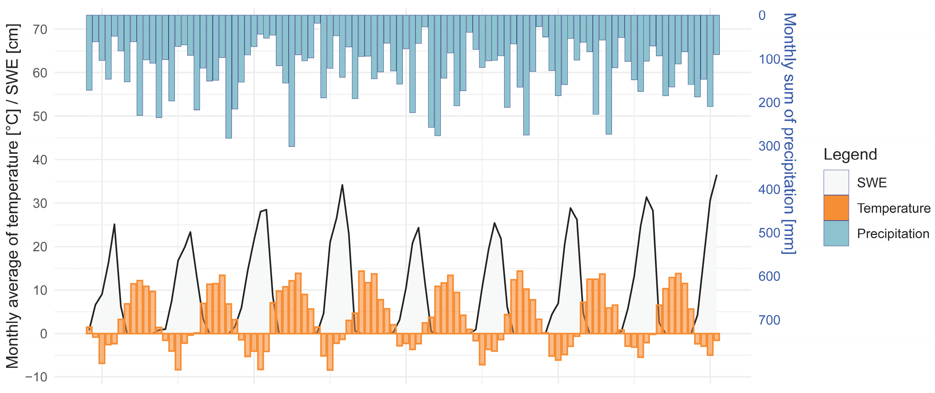
Precipitation and air temperature data have been recorded at the Červenec site since 1988, resulting in a 30-year continuous data series. The average annual precipitation is 1450 mm, with extremes recorded in 2003 (1086 mm) and 2010 (1984 mm). The average yearly air temperature during the observed period was 3.0 °C, with 8.7 °C in the warm half of the year (April to September) and −2.8 °C in the cold half (October to March). The variance of the mean monthly temperatures is shown in Figure 2. Air temperature was measured directly at the site.

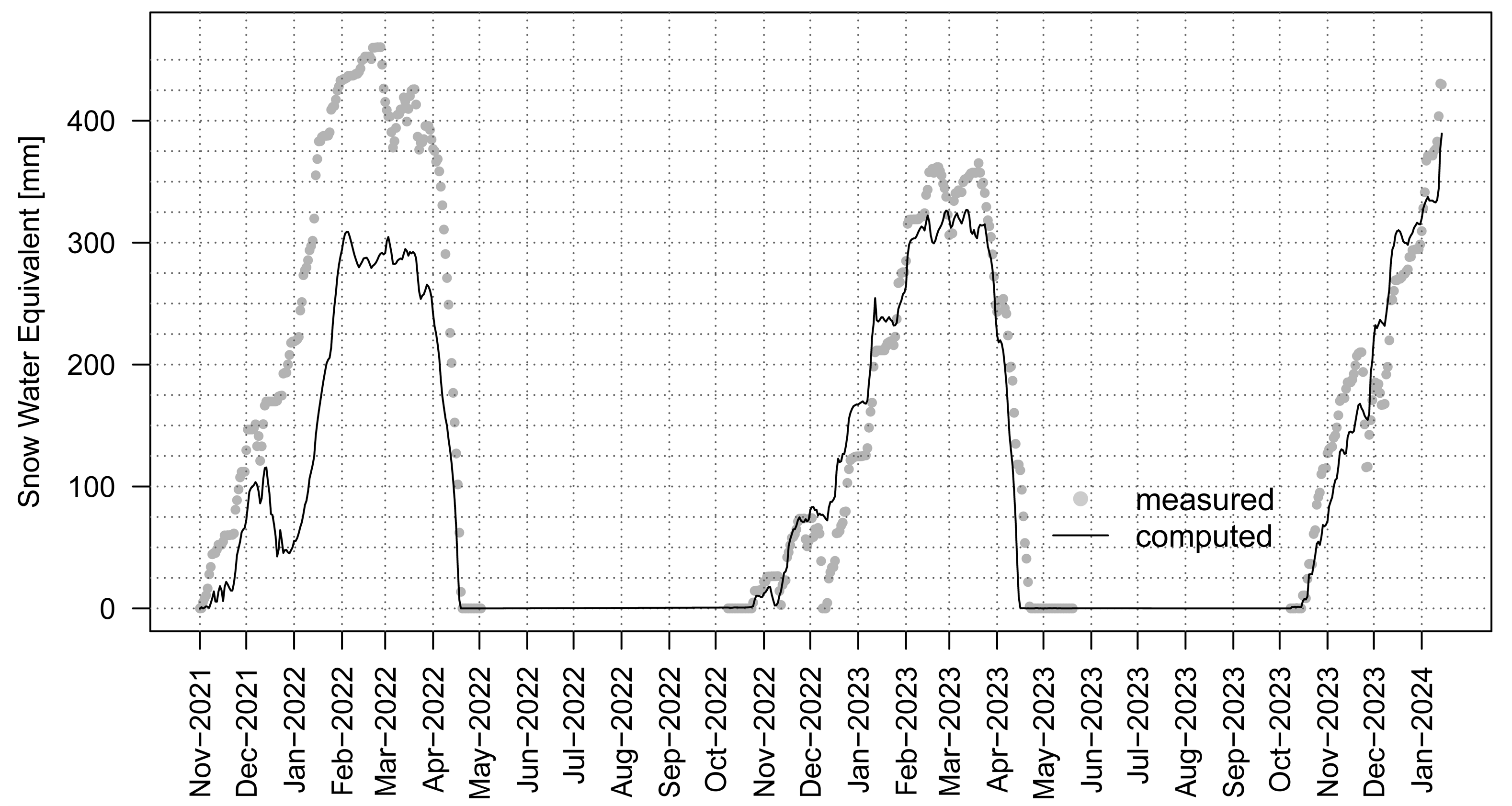
For this study, data used to assess snow water equivalent were collected from automatic snow measurements from 2016 to 2024 using a snow measuring scale (Sommer SSG-2, area: seven panels of 80 × 120 cm = 6.72 m², accuracy: 0.3%). The motivation for SWE modeling in this work is to obtain models capable of filling in missing data (or whole periods, e.g., before the installation of measuring devices or future periods). The snow seasons used in this study are shown in Figure 3.

The available data, collected using consistent measurement methods, was organized into a table. Following the standard practice recommended in the literature, the data was divided into a training set and a test set in a ratio of approximately 2:1. The training set covered the period from winter 2016 to 2021 and consisted of 1174 rows of data. The table columns represented the date, precipitation, temperature, and measured SWE. The test set encompassed the winters from 2022 to 2024 and included 506 rows of data. Models for SWE prediction were developed using the training data, and their performance was assessed using the test data.

3. Methods

The degree-day (DD) method [14] is widely used to estimate snow water equivalent. This method calculates snow accumulation and melting using daily air temperature and precipitation data. The DD method is based on the principle that snow accumulation occurs when the temperature is below a certain threshold (Tra), and snowmelt occurs when the temperature exceeds another threshold Trm. The transient tolerance Tr is used to evaluate the conditions under which the snow accumulates partially. The degree-day method can be described as follows (see Figure 4).

• Snow accumulation: When the air temperature (T_air) is below a specified threshold (Tr_a − Tr), all precipitation (P) falls as snow. If the temperature is between (Tr_a − Tr) and (Tr_a + Tr), a fraction of the precipitation falls as snow. If the temperature exceeds (Tr_a + Tr), no snow accumulates.
• Snowmelt calculation: When the air temperature exceeds a base temperature (Tr_m), snowmelt occurs at a rate proportional to the temperature difference (T_air − Tr_m). The proportionality constant is the degree-day factor (DDF). In this work, each month of the year has a specific value of DDF.

The DDFs are crucial to this method’s solution and were optimized in the following way. The data set (Date, T_air, P, SWE_observed) was divided into training and test sets. The training data was used to optimize each month’s DDF using a genetic algorithm (GA). The GA searches for the optimal set of DDFs by minimizing the root mean square error (RMSE) between the observed and simulated SWE values on training data. This work used monthly values of SWE, e.g., one value for every month in which snow cover occurs during some season of training data. The R package rgenoud was used for GA application [15].

The optimization begins with defining the search space for the DDFs (the range of possible values). These are between 0 and 8. The GA then selects a random initial population within this range (set of chromosomes). The fitness of each solution (chromosome) is evaluated using the RMSE between the observed and simulated SWE. GA iteratively evolves the population by selecting the best-performing individuals (chromosomes) and applies genetic operators such as crossover or mutation to create new solutions. This process continues until the fitness improvement stops, indicating convergence.

Once the optimal DDFs were identified, they were applied to the test data to simulate SWE. The degree-day function programmed by authors in R uses daily temperatures and precipitation as inputs and optimized monthly DDFs to calculate SWE. The model’s performance was evaluated by comparing the simulated SWE with the observed SWE values using various metrics.

3.1. Machine Learning Methods

The study used several machine learning methods to estimate SWE: simple linear regression, regularized linear regression (LASSO), Random Forest, Support Vector Regression, and CatBoost. These methods were chosen to represent different classes of machine learning algorithms. The study aimed to show whether more advanced techniques are required for the task or whether simpler methods, such as linear regression, could suffice.

The mathematical details of the machine learning algorithms are omitted in the following description, as they can be found in the references cited. Instead, the following text very briefly overviews the main features of used ML methods intended for non-professionals in data science.

• Multiple Linear Regression (MLR) addresses the linear relationship between independent and dependent variables. This basic approach serves as a comparison with other, more robust methods in this work. The MLR is defined in the following way:

Y = β₀ + β₁·X₁ + β₂·X₂ + … + β_p·X_p + ε

(1)

where Y is the dependent variable, X₁, X₂,…, X_p are the independent variables, β₀ is the intercept term, β₁, β₂,…, β_p are the coefficients, and ϵ is the error term. The most important task is to specify the coefficients calculated using the least squares method.

• LASSO Regression: LASSO (Least Absolute Shrinkage and Selection Operator) is a regularization method that helps prevent overfitting by shrinking the coefficients of less important variables towards zero [16]. In addition to using the previous equation, it introduces a penalty:

∑|β_i| ≤ λ

(2)

where λ is the tuned parameter and controls the amount of shrinkage. LASSO leads to simpler models with better generalization on unseen data than basic MLR.

• Support Vector Regression (SVR): SVR addresses nonlinear regression tasks using the kernel trick [17]. This approach involves mapping the data into a higher-dimensional space, making it a linear problem that is easier to solve. SVR then effectively captures the complex relationships that are not apparent in the original lower-dimensional space. Different kernels can be used, such as linear, polynomial, or radial basis function (RBF); the authors used the RBF kernel in this paper. Another key feature of SVR is introducing an error limit, denoted as ϵ. This error limit helps avoid overfitting by allowing the algorithm to ignore errors within a specified margin ϵ (the tuning parameter). The algorithm aims to find an ML model that deviates from the actual data points by no more than ϵ. This approach balances the model’s complexity and ability to generalize on unseen data.
• Random Forest (RF): RF is a bagging ensemble of regression trees [18]. It constructs many regression trees in parallel and outputs their average prediction. A fundamental feature of the RF is bootstrap sampling, also known as bagging. Bootstrap sampling involves random selection of the subsets of the training data with replacement to train trees in the forest. Each tree is, therefore, trained on slightly different data, introducing diversity into the RF ensemble. As a result, the trees in the forest are not identical, and they do not all make the same mistakes. This diversity among the trees is crucial for the robustness of the RF model (reducing overfitting, reducing errors, and improving stability—less sensitivity to outliers).
• CatBoost: CatBoost is a regression-tree-based gradient boosting algorithm for numerical and categorical data [19]. It constructs an ensemble of sequential decision trees, a strategy different from bagging in RF. Each new tree aims to correct the errors made by the earlier version of the model (i.e., minimize the differences between the actual and predicted values) and iteratively refines the model in such a way.CatBoost incorporates several sophisticated strategies to prevent overfitting, such as ordered boosting, random permutations, L2 regularization, and bootstrap sampling. Ordered boosting processes capture data sequentially, ensuring that each data point is only used once, which prevents overfitting. By applying multiple random permutations of the training data, CatBoost also reduces overfitting and ensures that the model is exposed to diverse data subsets during training, increasing its generalization ability. CatBoost employs regularization, which adds a penalty based on the magnitude of the model’s coefficients. This helps prevent the model from fitting the noise. CatBoost uses bootstrap sampling like the RF to create diverse training subsets.
  A notable feature of CatBoost is its efficiency and ease of use. The algorithm comes with well-optimized default parameters, making it accessible to users who may not have extensive expertise in tuning machine learning models.

3.2. Feature Engineering

The original contribution of this work lies in the innovative use of feature engineering (FE) to refine SWE estimation models. FE transforms raw data into more informative features to improve the performance of ML models. Several strategies for FE have been proposed hereinafter for SWE estimation. These strategies enhance the model’s ability to capture relevant patterns in the data, leading to more accurate predictions.

Feature engineering is based on the temperature and precipitation data. So, there is no necessity for additional historically measured data. The following feature engineering transformations were applied to these data:

• SWE_Diff. The dependent variable was set as the difference between SWE on the current and previous day. Such a target variable is less dependent on the history of snow cover formation in a given location.
• Degree day variable. The degree day variable was calculated to quantify the heat accumulation critical for snowmelt. The threshold temperature for this process (Tr_m) was set to 0 °C. For each day, the degree day was computed as follows:

DD_i = max(T_{air, i} − Tr_m, 0)

(3)

where T_{air, i} is the temperature on day i. If it is below 0 °C, it is set to zero.

• Month variable. The month was extracted from each date in the dataset and converted into a categorical variable to address the seasonal effects on SWE. Creating individual models for every season helps in SWE modeling.
• Day of the season. A new variable, seasonDay, was created to represent the number of days since the season’s first snow. For each day i, this variable is calculated as follows:

seasonDay_i = Day_i − startDay_{ave_train} + 1

(4)

where startDay_{ave_train} is the average first day of snow season extracted from training data.

• Snow accumulation A_snow, melting M_snow and SWE_DD based on the Degree-Day Method. All calculations were performed according to the procedures described in the previous section on the degree-day method. A variable for the difference in SWE estimated by the degree-day method (SWE_difDD) was also calculated for each day:

SWE_{difDD, i} = SWE_{DD, i} − SWE_{DD, i−1}

(5)

• Liquid precipitation. The liquid component of the precipitation directly impacts snowmelt and SWE. It was calculated by subtracting the snow accumulation from the total precipitation:

Rain_i = Z_i − Asnow_i

(6)

where Z_i is the total daily precipitation, and Asnow_i is its snowfall part.

• Lagged temperature variables. Several lagged temperature variables were introduced to capture the temporal dependencies and delayed effects of temperature on snowmelt. These included the daily temperatures lagged by one to ten days.

T_{lag, k} = T_{air, i−k} for k = 1, 2, …, 10

(7)

• An average of these lagged temperatures was also computed over ten days (lagT_{1_10}):

$${\mathrm{T}}_{\mathrm{lag}, 1-10}={\displaystyle \frac{1}{10}}\sum _{\mathrm{k}=1}^{10}{\mathrm{T}}_{\mathrm{air}, \mathrm{i}-\mathrm{k}}$$

(8)

• Solar radiation. This variable provides insights into the potential solar energy available for snowmelt. The following equations calculate clear-sky solar radiation R_so [20]:

$$\mathrm{R}\mathrm{a}=(24·60/\mathsf{\pi })·\mathrm{G}\mathrm{s}\mathrm{c}·\mathrm{d}\mathrm{r}·\left(\mathrm{c}\mathrm{o}\mathrm{s}\right(\mathsf{\phi })·\mathrm{c}\mathrm{o}\mathrm{s}(\mathsf{\delta })·\mathrm{s}\mathrm{i}\mathrm{n}(\mathrm{w}\mathrm{s})+\mathrm{w}\mathrm{s}·\mathrm{s}\mathrm{i}\mathrm{n}(\mathsf{\phi })·\mathrm{s}\mathrm{i}\mathrm{n}(\mathsf{\delta }\left)\right)$$

(9)

R_so = (0.75 + 2 · 10⁻⁵ · z) · R_a

(10)

where R_so is the clear-sky solar radiation (in MJ/m²/day), z is the altitude above sea level (in meters), R_a is the extraterrestrial radiation on a horizontal surface (in MJ/m²/day), G_sc is the solar constant (0.0820 MJ/m²/min), d_r is the relative inverse Earth–Sun distance, φ is the latitude (in radians), δ is the solar declination (in radians), and w_s is the sunset hour angle (in radians).

• Gridded data. Currently, climatic data is available in regular grid form for nearly every location on Earth. Although grid data may be less accurate than data from point measurements, they can significantly improve machine learning accuracy if some variables are not routinely measured in a given area. Time series of air humidity and global radiation were taken from near grid points (Figure 5) of the European Climate Assessment & Dataset (ECA&D) [21]. Missing values in the ECA&D data were filled in using linear interpolation to ensure completeness of the data.

3.3. Fine-Tuning and Evaluation of Machine Learning Models

Fine-tuning involves configuring specific parameters that direct the behavior of particular ML algorithms. This process was carried out by searching for the optimal value of such parameters using k-fold cross-validation while assessing performance with various sets of tuning parameters. K-fold cross-validation involves dividing the training data into k folds, training the model k times, and using different folds for testing each time. The optimal parameters were selected based on the best RMSE value.

The model’s performance was assessed on test data using Mean Error (ME), Root Mean Square Error (RMSE), Percentual Bias (PBIAS), Nash–Sutcliffe efficiency (NSE), and the Coefficient of Determination (R²). All these well-known characteristics are described in standard scientific literature and in the vignette of the R package hydroGOF, which was used for evaluations.

The tuning and evaluation process was programmed and conducted in the R language environment using R packages such as caret [22], parallel [23], registerDoParallel, hydroGOF [24], glmnet [16], randomForest [25], CatBoost [19], kernlab [26], and h2o [27]. Testing data was not used during parameter calibration.

4. Results

The study compared traditional and machine learning methods for predicting SWE. A more precise method than the standard approach was being sought. This section evaluates the proposed ML algorithms’ performance with regards to this aim. The purpose of choosing more algorithms was twofold: firstly, to consider the ‘no free lunch’ theorem (one does not know in advance which algorithm is best suited for a given task) and to determine whether advanced algorithms are necessary or whether simpler models might be sufficient.

4.1. Data Preprocessing

The relevant previous section describes the base, raw data used (time series of climatic measurements). Various operations have been applied to the raw data, including those proposed by the authors, to achieve better results from the modeling.

Missing data occurred only for the humidity variable from the ECA&D database. Simple linear interpolation was used to fill gaps because the missing data periods were short, making a more sophisticated imputation method unnecessary.

Feature engineering. Various algebraic and physically based construction methods were used, which generated new variables—features. This step of data preprocessing greatly influences the effectiveness of the subsequently used models and is considered a crucial part of the proposed methodology. The methodology of generating features is described in the Methodology section, and the list of features is recapitulated in

Table 1. Features used in this study.

Variable Name	Min	Max	Mean	Correlation Coefficient with “Dif”	Description
dif	−55.78	50.40	0.25	1	SWE daily increment
Tair	−21.23	13.54	−1.75	−0.40	temperature
Z	0.00	51.43	3.87	0.30	precipitation
DD	0.00	13.54	1.44	−0.42	degree day
month	1.00	8.00	-	-	month (categorical variable)
seasonDay	1.00	224.00	97.03	−0.27	day of the snow season
SWE_DD	0.00	488.42	157.52	0.05	SWE computed by DD
Asnow	0.00	51.43	3.49	0.33	accumulation of snow by DD
Msnow	0.00	54.16	3.24	−0.52	melt of snow by DD
bilDay	−54.16	41.43	0.45	0.58	Asnow—Msnow
rain	0.00	43.74	0.38	−0.15	liquid part of precipitation
lagDD1	0.00	13.71	1.44	−0.38	lagged degree day by 1 day
lagDD2	0.00	13.71	1.44	−0.26	lagged degree day by 2 day
lagDD3	0.00	13.71	1.44	−0.18	lagged degree day by 3 day
lagDD1_10	0.00	10.00	1.45	−0.21	average of last 10 DDs
Rso	6.18	32.49	13.96	−0.31	daily value of solar radiation
hu	33.85	95.20	80.00	0.19	humidity from ECA&D
qq	0.00	366.00	87.59	−0.29	global radiation from ECA&D

.

Some of the proposed variables may be mutually correlated, which may cause the creation of less stable models. For this reason, a correlation analysis was performed. The results are summarized in Figure 6, in which the absolute values of correlation coefficients for all pairs of variables are evaluated.

The correlation coefficients ranged from 0.003 to a 0.97. A high mutual correlation between independent variables is not desirable, and the more suitable explanatory variable should correlate better with the dependent variable—daily SWE increment (dif). An absolute value of correlation greater than 0.85 was considered as high. Based on these principles, total precipitation Z was excluded from inputs. Its correlation coefficient with the snow accumulation variable (Asnow) is 0.93. Asnow better correlated with the dependent variable than Z (0.30 versus 0.36), so it was Z from these two variables which was excluded from the inputs. Similarly, the variable order of the day in the snow season (seasonDay), which correlated with solar radiation (Rso) with a correlation coefficient of 0.87, was also excluded. Variable SWE based on the degree-day method (SWE_DD) was also excluded from inputs due to low correlation with the dependent variable (r = 0.05).

Interaction of variables. Interaction terms were created by multiplying two variables together. This captures the combined effect of these variables on the calculated SWE, which may provide more helpful information than using variables separately (synergy effect). For example, while individual variables such as temperature and precipitation have some effects on SWE, their combined impact can often provide more valuable insights. This approach can capture nuances in snowfall patterns that are not apparent when only examining variables separately, leading to more accurate and reliable SWE predictions. The analysis in Figure 7 examines the usefulness of including interactions between variables. It shows a list of variables on the x and y axes, and the x and y intersections represent the product of the variables. The color of the corresponding square in this intersection indicates the absolute value of the correlation coefficient between the mentioned product of variables and the dependent variable (dif), as shown in the legend. The variables Rso*DD, Rso*Msnow, and Rso*lagDD1_10 were added to the inputs based on Figure 7. This was performed based on the adopted principle that a new, interacting variable will be accepted into the input data only if its correlation coefficient (absolute value) is greater than it was for the original variables.

4.2. Evaluation of the Degree-Day Method

The degree-day method serves as the standard for comparison with other methods. This work used degree-day factor optimization, a key parameter in this method, employing a genetic algorithm (GA). Optimization involves selecting/programming a proper GA algorithm, defining the chromosome (which encodes the parameters to be optimized), and programming the fitness function to evaluate each proposed solution coded in a chromosome. The authors have chosen the Genoud algorithm [15]. The Methodology section details the fitness function, which is the degree-day algorithm. The chromosome comprises a degree-day factor for each month and three constants: thresholds for snowmelt (Trm) and accumulation (Tra) and a transition interval Tr (Figure 4). Besides the temperature and precipitation time series necessary during the training period, the optimization process also requires the measured values of SWE to calculate the fitness function value for each chromosome, namely, the RMSE. The GA aims to find the chromosome which has the best fitness function value, obtained by evolving chromosomes with operators inspired by evolution.

Figure 8 shows the results obtained for the test data. The test statistics for the degree-day method are RMSE = 79.46, PBIAS = 27.2%, NSE = 0.57, and R² = 0.8. This work aims to improve the test statistics’ values with the proposed methods evaluated later in this text. The smaller NSE and large RMSE and PBIAS values indicate relatively weaker results. For comparison, these results are in

Table 2. Evaluation of SWE calculation by ML with raw data.

Statistic	Degree Day	MLR	LASSO	CatBoost	Random Forest
ME	41.64	−29.34	−30.08	−6.10	−19.75
RMSE	79.46	85.79	86.02	67.67	75.92
PBIAS %	27.20	−19.20	−19.70	−4.00	−12.90
NSE	0.57	0.49	0.49	0.69	0.60
R2	0.80	0.56	0.56	0.69	0.63

, together with results from the proposed ML methods.

4.3. Evaluation of Machine Learning Methods for SWE Computation

The following solution alternatives were evaluated:

• ML without feature engineering using MLR, LASSO, RF, SVM, and CatBoost (i.e., solely with raw data);
• ML with feature engineering using the same machine learning methods.

The input data varied for different calculations, and the calculated variable was always the daily increment/decrement of the SWE value. This approach is preferable to directly calculating the SWE value, as this dependent variable is less influenced by climate history in the current snow season. The resulting daily SWE values were calculated by summing the previous daily SWE increments (see Figure 9).

All machine learning calculations were carried out using the R language environment [23]. The computational runs varied in duration, from a few seconds for simpler methods to several minutes, with a maximum of about 10 min. These computations mainly aim to determine the specific parameters for each algorithm, which are different for each particular task. Cross-validation was consistently employed for this purpose. Authors intentionally do not provide details, such as the progress and final values of the parameters computed in this way, due to the smoother flow of the text. Still, the following part constituted the main content and volume of work due to the extensive programming required in R and the execution and evaluation of the computations.

4.3.1. Calculation of SWE by Machine Learning Using Raw Data

ML models described in the Methodology section were used to calculate the SWE. The inputs to these models were precipitations and temperatures, and the dependent variable was the daily increment/decrement of SWE recalculated subsequently, according to Figure 9 to SWE.

In Figure 10 and Table 2, the evaluation and comparison of four machine learning models using the degree-day method show that the machine learning model selection is essential. Only one (CatBoost) performed better than the degree-day method when using raw data without applying feature engineering. However, even the CatBoost model did not outperform the degree-day method regarding the coefficient of determination; its value was worse (0.69 versus 0.80). However, all other indices showed a better result for the CatBoost algorithm than the degree-day method.

4.3.2. Calculation of SWE by Machine Learning Using Features

The inputs to models in this section were features listed in Table 1, and the dependent variable was again the daily increase/decrease in SWE.

In Figure 11 and

Table 3. Evaluation of SWE calculation by ML with features listed in Table 1.

Statistic	Degree Day	MLR	LASSO	CatBoost	Random Forest
ME	41.64	1.69	3.44	6.79	6.28
RMSE	79.46	53.05	51.35	45.64	47.93
PBIAS %	27.20	1.10	2.30	4.40	4.10
NSE	0.57	0.81	0.82	0.86	0.84
R2	0.80	0.81	0.82	0.86	0.84

, the evaluation and comparison of four machine learning models using the degree-day method show that machine learning with feature engineering is essential to the quality of the computation results. All algorithms work better in this case than the degree-day method and machine learning with raw data. The Catboost algorithm again provides the best results, and all algorithms are better in all indicators than the result from the previous section, e.g., higher coefficients of determination and Nash–Sutcliffe coefficient of efficiency and lower ME, RMSE, and PBIAS.

5. Discussion

The paper presents a study that compares proposed ML algorithms with traditional methods for estimating SWE in a mountainous region of Slovakia. The results highlight the potential of ML techniques, particularly CatBoost, in improving the accuracy of SWE predictions compared to the conventional degree-day model. The paper builds on previous works in this area (e.g., [28]) and confirms the benefits of using more advanced machine learning methods. Both ensemble methods—a Random Forest that uses bagging (results of which are averaged predictions of multiple parallel predictors) and CatBoost which is using boosting (which involves the stepwise improvement of the predictions by successive models)—provided better results than the simpler linear models.

Comparison of the evaluations in Table 2 and Table 3 highlights the importance of this paper’s main innovation—proposed feature engineering methods, which significantly improved the accuracy of SWE forecasts. This element brings a symbiosis of hydrological knowledge with the ML black boxes, as the design of features (mathematical combinations created from original variables) is based on knowledge of the physical processes behind the given problem. To the best of the authors’ knowledge, such computational experiments regarding FE in SWE modeling are not presented thoroughly in scientific literature. The effectiveness of the ML with feature engineering is indicated, e.g., by higher coefficients of determination, which increased from 0.8 to 0.86. Moreover, the Nash–Sutcliffe efficiency, reflecting the model’s ability to predict higher values, has risen from 0.57 to 0.86, which is a significant improvement (compare Figure 10 and Figure 11). Lower error metrics such as RMSE and PBIAS also reflect better variance and lower systematic errors in SWE predictions when using ML with FE. This also indicates the importance of leveraging feature engineering techniques to improve the accuracy of hydrological forecasts in general. It is up to the problem solvers and their familiarity with the problem to design appropriate transformations of raw variables into features which will be helpful for a given task (or a paper, like this one, can serve as a guide).

The authors also evaluated individual features’ suitability, as shown in Figure 12. This figure illustrates the importance of variables in calculating the target value (the SWE daily increment). This importance is based on the internal mechanism of the individual algorithms and is available as their output. The x-axis of Figure 12 displays the variable names (according to the abbreviations in Table 1) sorted by their importance in the CatBoost algorithm, the most effective algorithm. Figure 12 shows that the four constructed features are more important for the calculation than any original variable (the fifth is T_air—air temperature). Successful algorithms like CatBoost and Random Forest show similar variable importances, whereas linear regression exhibits significant differences. A more accurate algorithm can also determine the importance of variables more realistically. Consequently, the most important variable is bilDay, which represents the daily balance of snowmelt and snowpack formation obtained through the simple balance principles described in the Methods section. This result is also obvious through physical reasoning.

However, there are also some challenges associated with the use of ML in SWE estimation. One notable concern is the “black box” reputation of ML algorithms, which can make it difficult to interpret the underlying mechanisms driving the predictions [29]. This lack of interpretability limited the scientists’ and stakeholders’ ability to fully trust the model’s outputs. However, this problem is currently being intensively researched (e.g., [30]) and we tried to deal with this issue to a limited extent in this article as well; see Figure 12, which analyzes the influence and thus the meaning of individual variables used for modeling. There is also a risk of overfitting [31], where the model performs well on training data but fails to generalize effectively to new, unseen data. In the present article, the authors tried to limit this risk by reducing some variables based on their mutual correlations (see Figure 7). Furthermore, ML models are computationally intensive and may require significant computational resources for training and inference, which could be a limitation for some applications.

Future research in this field could explore the scalability and transferability of ML models to different geographical locations and climatic conditions and address various challenges in water resources management. As some other works on this issue [32,33] have stated, different data obtained by remote sensing are more suitable for this purpose than point data sources used in this work. The methodology proposed in this work may be used by map algebra to refine the results [34].

6. Conclusions

This study demonstrates the benefits of using machine learning (ML) algorithms over traditional methods for estimating snow water equivalent (SWE) in mountainous areas. It emphasizes the potential of ML techniques to enhance the accuracy of SWE predictions. The study revealed that machine learning models, particularly CatBoost with feature engineering (FE), significantly outperformed the traditional degree-day method in the presented case study in terms of predictive accuracy and reliability. Creating new variables by FE was originally proposed by authors and based on knowledge of the physical processes of melting and snow cover formation. The modeling results were significantly improved. Unlike the ML models, which used two basic, measured climatic variables (i.e., raw data), these models contained 16 variables derived from these two variables and two variables available potentially everywhere. The accuracy of modeling SWE was enhanced when using FE—the Nash–Sutcliffe efficiency value, reflecting overall accuracy as well as extreme value modeling accuracy, was 0.57 in the presented study with the traditional degree-day method but improved to 0.69 with ML methods utilizing raw data (temperature, precipitation). Finally, it increased to 0.86 with the CatBoost model and new computationally derived (not measured) variables gained by feature engineering. An important insight from this study is that for the successful use of machine learning, not only the choice of an algorithm but also the creative work of the solver, an expert in hydrology who can provide know-how in analyzing and preprocessing data sources, is essential.

The successful application of ML algorithms in SWE estimation holds promising prospects for hydrological modeling and water resource management in snow-dominated regions. By harnessing advanced computational techniques and integrating FE, researchers can enhance the precision of SWE forecasts, enabling informed decision-making in water allocation, flood risk assessment, and ecosystem management.

References

- Ma, Y.; Huang, Y.; Chen, X.; Li, Y.; Bao, A. Modelling Snowmelt Runoff Under Climate Change Scenarios in an Ungauged Mountainous Watershed, Northwest China. Math. Probl. Eng. 2013, 2013, 1–9. [Google Scholar] [CrossRef]
- Brown, R.D.; Mote, P.W. The Response of Northern Hemisphere Snow Cover to a Changing Climate. J. Clim. 2009, 22, 2124–2145. [Google Scholar] [CrossRef]
- DeWalle, D.R.; Rango, A. Principles of Snow Hydrology; Cambridge University Press: Cambridge, UK, 2008; ISBN 1139471600. [Google Scholar]
- Butt, M.J.; Bilal, M. Application of Snowmelt Runoff Model for Water Resource Management. Hydrol. Process. 2011, 25, 3735–3747. [Google Scholar] [CrossRef]
- Zhang, Y.; Liu, S.; Ding, Y. Observed Degree-Day Factors and Their Spatial Variation on Glaciers in Western China. Ann. Glaciol. 2006, 43, 301–306. [Google Scholar] [CrossRef]
- Martinec, J. The Degree-Day Factor for Snowmelt-Runoff Forecasting; IAHS Publication: Wallingford, UK, 1960; Volume 51, p. 468. [Google Scholar]
- Dawson, C.W.; Wilby, R.L. Hydrological Modelling Using Artificial Neural Networks. Prog. Phys. Geogr. Earth Environ. 2001, 25, 80–108. [Google Scholar] [CrossRef]
- Wang, G.; Hao, X.; Yao, X.; Wang, J.; Li, H.; Chen, R.; Liu, Z. Simulations of Snowmelt Runoff in a High-Altitude Mountainous Area Based on Big Data and Machine Learning Models: Taking the Xiying River Basin as an Example. Remote Sens. 2023, 15, 1118. [Google Scholar] [CrossRef]
- Zhang, J.; Pohjola, V.A.; Pettersson, R.; Norell, B.; Marchand, W.-D.; Clemenzi, I.; Gustafsson, D. Improving the Snowpack Monitoring in the Mountainous Areas of Sweden from Space: A Machine Learning Approach. Environ. Res. Lett. 2021, 16, 084007. [Google Scholar] [CrossRef]
- Vafakhah, M.; Nasiri Khiavi, A.; Janizadeh, S.; Ganjkhanlo, H. Evaluating Different Machine Learning Algorithms for Snow Water Equivalent Prediction. Earth Sci. Inform. 2022, 15, 2431–2445. [Google Scholar] [CrossRef]
- Thapa, K.K.; Singh, B.; Savalkar, S.; Fern, A.; Rajagopalan, K.; Kalyanaraman, A. Attention-Based Models for Snow-Water Equivalent Prediction. In Proceedings of the AAAI Conference on Artificial Intelligence, London, UK, 20–27 February 2024; Volume 38, pp. 22969–22975. [Google Scholar] [CrossRef]
- De Gregorio, L.; Günther, D.; Callegari, M.; Strasser, U.; Zebisch, M.; Bruzzone, L.; Notarnicola, C. Improving Swe Estimation by Fusion of Snow Models with Topographic and Remotely Sensed Data. Remote Sens. 2019, 11, 2033. [Google Scholar] [CrossRef]
- Hsu, F.; Sun, Z.; Prathin, G.; Achan, S. A Review of Machine Learning in Snow Water Equivalent Monitoring. arXiv 2024. [Google Scholar] [CrossRef]
- Hock, R. Temperature Index Melt Modelling in Mountain Areas. J. Hydrol. 2003, 282, 104–115. [Google Scholar] [CrossRef]
- Mebane, W.R.; Sekhon, J.S. Genetic Optimization Using Derivatives: The Rgenoud Package for R. J. Stat. Softw. 2011, 42, 1–26. [Google Scholar] [CrossRef]
- Friedman, J.; Hastie, T.; Tibshirani, R. Regularization paths for generalized linear models via coordinate descent. J. Stat. Softw. 2010, 33, 1. [Google Scholar] [CrossRef] [PubMed]
- Awad, M.; Khanna, R.; Awad, M.; Khanna, R. Support Vector Regression. In Efficient Learning Machines; Apress: Berkeley, CA, USA, 2015; pp. 67–80. ISBN 978-1-4302-5989-3. [Google Scholar]
- Breiman, L. Random Forest. Mach. Learn. 2001, 45, 5–32. [Google Scholar] [CrossRef]
- Dorogush, A.V.; Ershov, V.; Gulin, A. Catboost: Gradient Boosting with Categorical Features Support: Gradient Boosting with Categorical Features Support. arXiv 2018. [Google Scholar] [CrossRef]
- Allen, R.G.; Pereira, L.S.; Raes, D.; Smith, M. FAO Irrigation and Drainage Paper No. 56. Rome Food Agric. Organ. United Nations 1998, 56, e156. [Google Scholar]
- Klein Tank, A.M.G.; Wijngaard, J.B.; Können, G.P.; Böhm, R.; Demarée, G.; Gocheva, A.; Mileta, M.; Pashiardis, S.; Hejkrlik, L.; Kern-Hansen, C.; et al. Daily Dataset of 20th-Century Surface Air Temperature and Precipitation Series for the European Climate Assessment. Int. J. Climatol. 2002, 22, 1441–1453. [Google Scholar] [CrossRef]
- Kuhn, M.; Wing, J.; Weston, S.; Williams, A.; Keefer, C.; Engelhardt, A. Classification and Regression Training; R Package Version 6.0-93; R Package Vignette: Madison, WI, USA, 2022. [Google Scholar]
- R Core Team. R: A Language and Environment for Statistical Computing. R Foundation for Statistical Computing; R Core Team: Vienna, Austria, 2013. [Google Scholar]
- Zambrano-Bigiarini, M. Hydrogof: Goodness-of-Fit Functions for Comparison of Simulated and Observed Hydrological Time Series; R Core Team: Vienna, Austria, 2022; pp. 1–77. [Google Scholar] [CrossRef]
- Liaw, A.; Wiener, M. Breiman and Cutler’s Random Forests for Classification and Regression: Breiman and Cutler’s Random Forests for Classification and Regression. R Package Version 2015, 4, 6–12. [Google Scholar]
- Karatzoglou, A.; Smola, A.; Hornik, K.; Zeileis, A. Kernlab–An S4 Package for Kernel Methods in R. J. Stat. Softw. 2004, 11, 1–20. [Google Scholar] [CrossRef]
- Fryda, T.; LeDell, E.; Gill, N.; Candel, A.; Click, C.; Kraljevic, T.; Nykodym, T.; Aboyoun, P. H2O: R Interface for the ‘H2O’ Scalable Machine Learning Platform: R Package Version 3.40.0.4; R Core Team: Vienna, Austria, 2023. [Google Scholar]
- Holko, L.; Danko, M.; Jančo, M.; Sleziak, P. Empirical models to calculate the snow water equivalent in the high mountain catchments of the Western Carpathians. Acta Hydrol. Slovaca 2022, 23, 241–248. [Google Scholar] [CrossRef]
- Eden, S.; Megdal, S.B.; Shamir, E.; Chief, K.; Mott Lacroix, K. Opening the black box: Using a hydrological model to link stakeholder engagement with groundwater management. Water 2016, 8, 216. [Google Scholar] [CrossRef]
- Núñez, J.; Cortés, C.B.; Yáñez, M.A. Explainable Artificial Intelligence in Hydrology: Interpreting Black-Box Snowmelt-Driven Streamflow Predictions in an Arid Andean Basin of North-Central Chile. Water 2023, 15, 3369. [Google Scholar] [CrossRef]
- Gharib, A.; Davies, E.G. A workflow to address pitfalls and challenges in applying machine learning models to hydrology. Adv. Water Resour. 2021, 152, 103920. [Google Scholar] [CrossRef]
- Sleziak, P.; Jančo, M.; Danko, M.; Méri, L.; Holko, L. Accuracy of radar-estimated precipitation in a mountain catchment in Slovakia. J. Hydrol. Hydromech. 2023, 71, 111–122. [Google Scholar] [CrossRef]
- Parajka, J.; Bezak, N.; Burkhart, J.; Hauksson, B.; Holko, L.; Hundecha, Y.; Jenicek, M.; Krajčí, P.; Mangini, W.; Molnar, P.; et al. Modis Snowline Elevation Changes During Snowmelt Runoff Events in Europe. J. Hydrol. Hydromech. 2019, 67, 101–109. [Google Scholar] [CrossRef]
- Krajčí, P.; Danko, M.; Hlavčo, J.; Kostka, Z.; Holko, L. Experimental measurements for improved understanding and simulation of snowmelt events in the Western Tatra Mountains. J. Hydrol. Hydromech 2016, 64, 316–328. [Google Scholar] [CrossRef]