

Research on the Development Height Prediction Model of Water-Conduction Fracture Zones under Conditions of Extremely Thin Coal Seam Mining

Abstract
1. Introduction
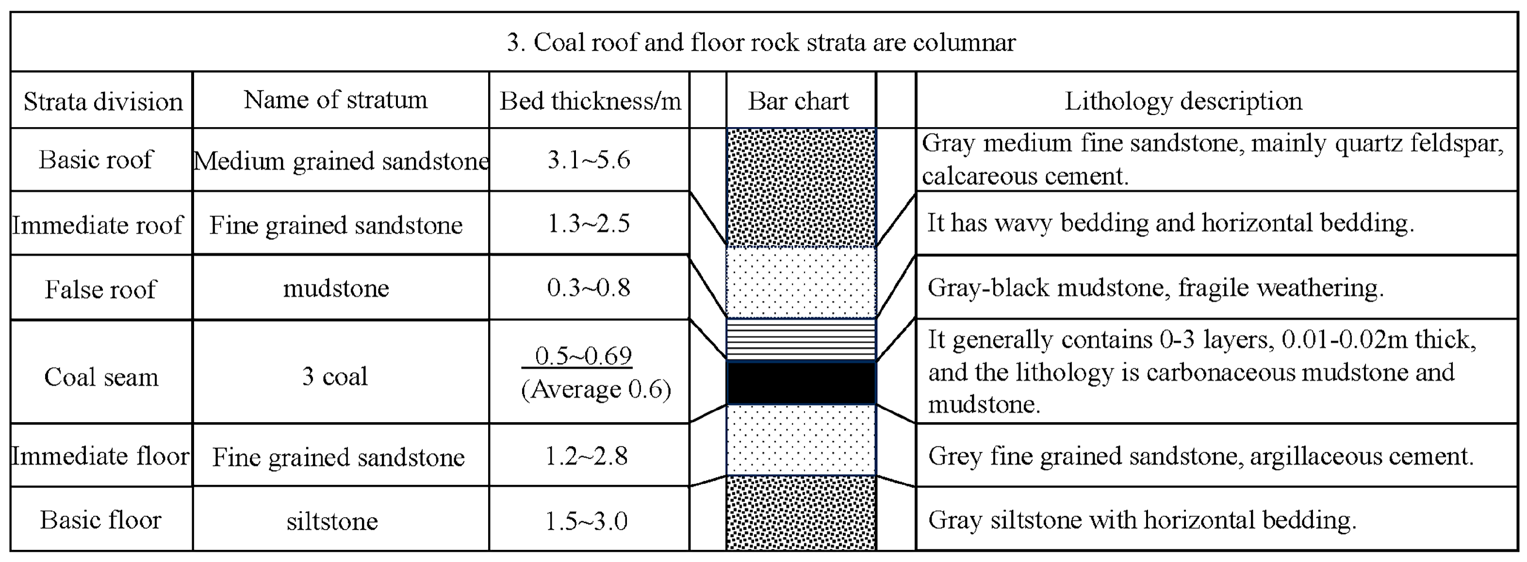
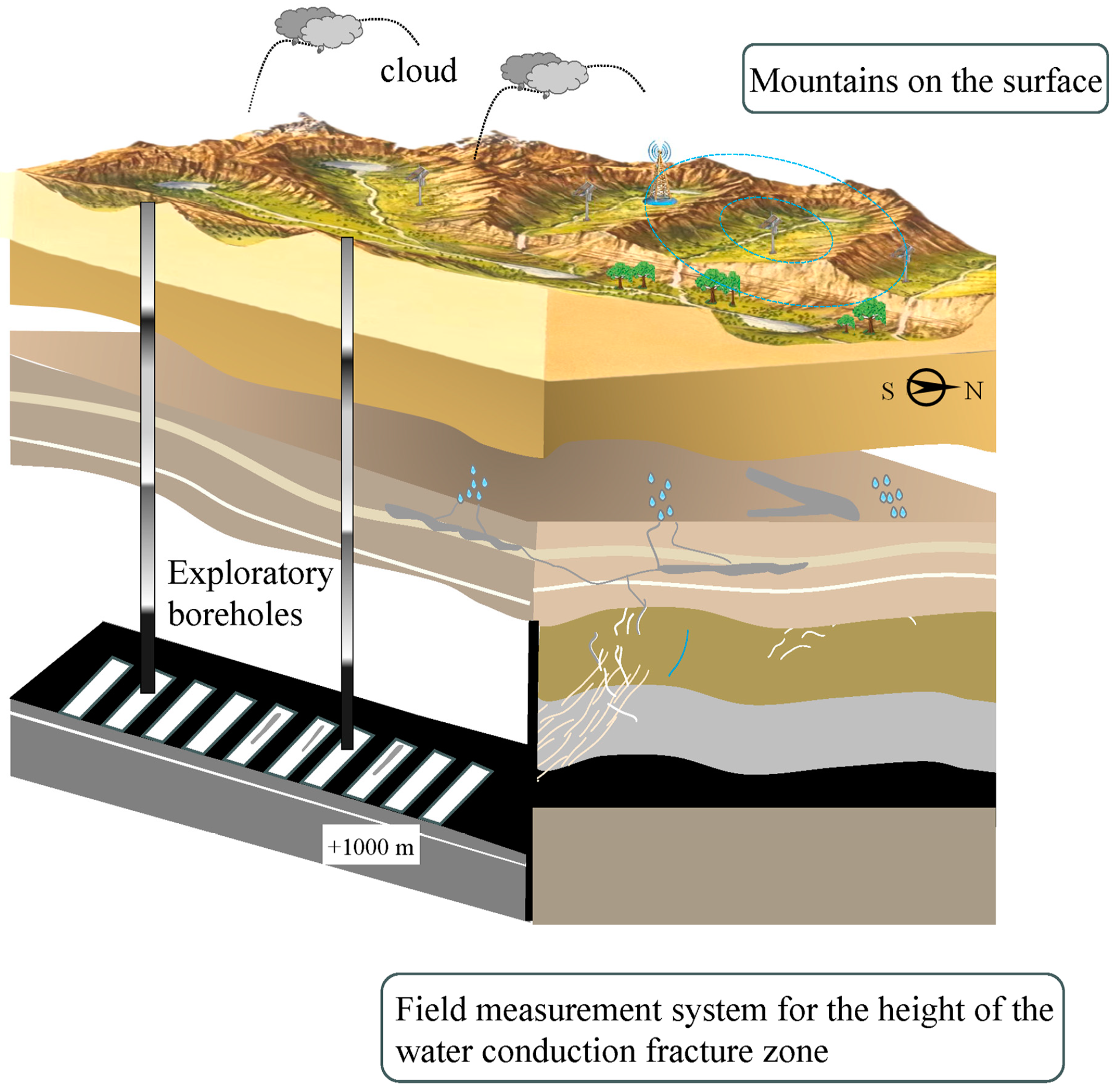
2. Project Overview
3. Construction of Data Set on the Height of the Water-Conduction Fracture Zone
3.1. Construction of the Index System of the Height of the Water-Conducting Fracture Zone
- (1)
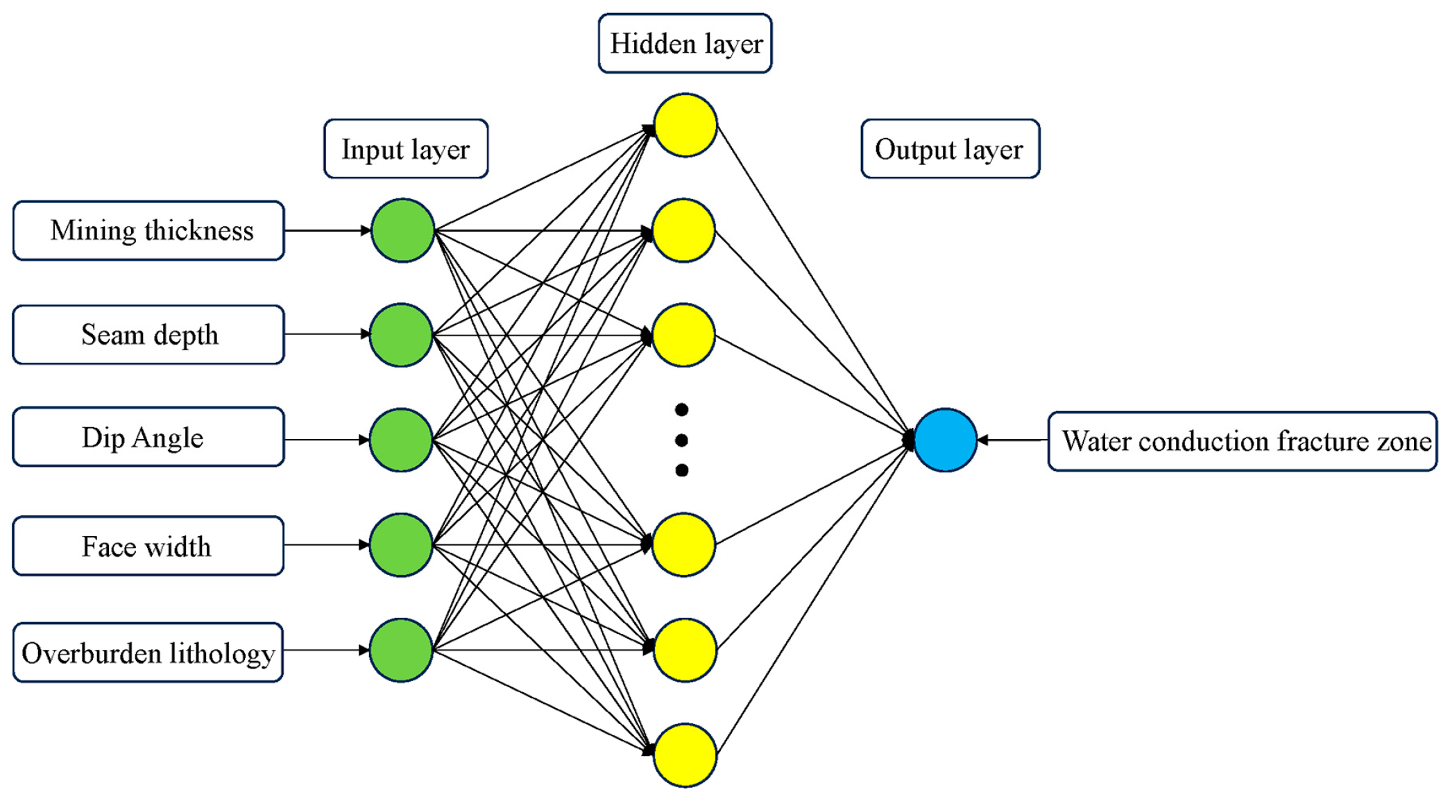
- Mining thicknessMining thickness affects the stress redistribution of roof strata and the failure range of overburden rock. It is the most critical factor for the failure of overburden rock and the development height of water-conducting fracture zones. In general, the greater the mining thickness, the higher is the height of the caving zone and water-conducting fracture zone, and the ratio is approximately linear [34].
- (2)
- Width of the working faceThe width of the working face, which refers to the inclined layout distance of the working face, is an influential factor in determining the size of the mining space affecting the water-conducting fracture zone and the area of the mining space. In the initial stage of coal seam mining, the height of the water-conducting fracture zone gradually increases with the increase in working face width [35].
- (3)
- Mining DepthThe buried depth of a coal seam alters the initial stress of overlying rock, leading to the failure of the overlying rock under compression, tension, and shear stress. The greater the buried depth of a coal seam, the greater is the stress on the overlying rock, leading to a corresponding increase in the degree of damage to the overlying rock [34].
- (4)
- Overburden LithologyThe development of mining fractures in overlying rock is closely related to the mechanical properties of the overlying rock, which determine the strength of the rock layer. Brittle rock layers are prone to fracturing, while plastic rock layers are more likely to bend and deform without developing fractures easily. The harder the rock layer, the greater is the height of overlying rock failure and the water-conducting fracture zone [34,35,36,37].
- (5)
- Coal Seam InclinationThe change in the inclination angle of a coal seam mainly affects the failure pattern of overlying rock. The water-conducting fracture zone of a horizontal coal seam has a saddle shape with high ends and a low middle. In contrast, the caving rock of an inclined coal seam fills the lower goaf due to gravity, resulting in the water-conducting fissure zone taking on an upper and lower shape [34].
- (6)
- Mining MethodsThe influence of the mining method on the height of the water-conducting fracture zone mainly depends on the size of the mining space and the movement form of caving rock in the goaf [37].
3.2. Data Set Construction
4. Multiple Regression Prediction Model
4.1. Modeling Analysis of Multiple Linear Regression Model
4.2. Modeling and Analysis of Multiple Regression Nonlinear Model
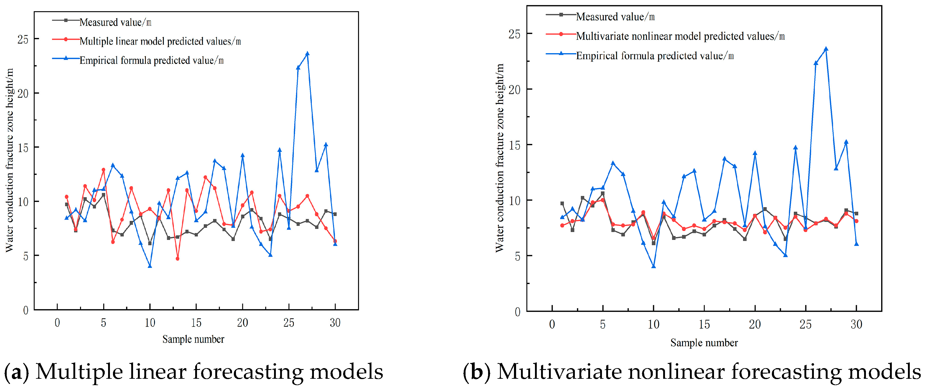
4.3. Verification of Multiple Regression Prediction Model
5. BP Neural Network Model
5.1. Construction of BP Neural Network Model
5.2. Network Learning and Training
5.3. Analysis of Prediction Results
5.4. Model Test
6. Application Example
7. Conclusions
- (1)
- The multiple regression linear model and the multiple regression nonlinear model of extremely thin coal seam show that the trend change between the measured value and the predicted value is consistent, and the error range is obviously reduced with the formula in the Three Gorges regulation, indicating that the regression prediction model is effective in predicting the height of the water-conducting fracture zone. It provides theoretical guidance for the field measurement of water-conducting fracture zones.
- (2)
- Through comparative analysis, multiple linear regression, multi-distance nonlinear regression, and BP neural network can all improve the prediction accuracy of the height of the water-conducting fracture zone. Among several prediction methods, the BP neural network had the best effect.
- (3)
- The BP neural network, multiple linear regression model, multi-distance nonlinear regression model, and traditional three-order empirical formula were compared to analyze their relative error and absolute error. The BP neural network has good fault tolerance by using “error backpropagation”, reducing the correlation between factors and improving the degree of model prediction. Moreover, the prediction accuracy of the BP neural network is as high as 93%, and the predicted result is basically consistent with the real value, which proves the accuracy of the model, and the application effect is good. This method can be used to predict the height of mine water-conduction fracture zones and guide mine safety production.
- (4)
- Since there is limited research on mining extremely thin coal seams both domestically and internationally, the height of the water-conducting fracture zone will be influenced by various factors during coal seam mining. Since our research focuses on a single mining area, the considered factors are relatively limited. In the future, it is advisable to explore additional influencing factors and conduct quantitative analysis using various modified optimal models. By doing so, the accuracy of the optimal model will be improved, providing a reference value for predicting the development height of water-conducting fracture zones under mining conditions of extremely thin coal seams.
Author Contributions
Funding
Data Availability Statement
Acknowledgments
Conflicts of Interest
References
- Gao, Y. “Four-belt” model of rock displacement and dynamic displacement inverse analysis. J. China Coal Soc. 1996, 51–56. [Google Scholar]
- Qian, M.; Xu, J.; Miao, X. Green mining technology of coal mine. J. China Univ. Min. Technol. 2003, 5–10. [Google Scholar]
- State Administration of Coal Industry. Regulations for Coal Pillar Retention and Coal Mining in Buildings, Water Bodies, Railways and Main Shafts and Lanes; Coal Industry Press: Beijing, China, 2000. [Google Scholar]
- Shi, L.Q.; Xin, H.Q.; Zhai, P.H.; Li, S.C.; Liu, T.B.; Yan, Y.; Wei, W.X. Research on height calculation of water-conducting fracture zone under large mining depth. J. China Univ. Min. Technol. 2012, 41, 37–41. [Google Scholar]
- Li, Z.; Xie, J.; Wang, F. Position and mining height are broken key stratum of abutment pressure influence law of the research and application. J. Coal Technol. 2015, 34, 34–36. [Google Scholar]
- Dong, Y.; Huang, Y.; Du, J.; Zhao, F. Study on Overburden Stability and Development Height of Water Flowing Fractured Zone in Roadway Mining with Cemented Backfill. J. Shock. Vib. 2021, 2021, 1–12. [Google Scholar] [CrossRef]
- Xu, J.; Zhu, W.; Wang, X. Based on the position of key stratum water fractured zone height is expected method. J. Coal 2012, 5, 762–769. [Google Scholar]
- Zha, H.; Liu, W.; Liu, Q. Physical Simulation of the Water-Conducting Fracture Zone of Weak Roofs in Shallow Seam Mining Based on a The Self-Designed Hydromechanical Coupling Experiment System. J. Geofluids 2020, 2020, 1–14. [Google Scholar] [CrossRef]
- Sun, D.; Li, X.; Zhu, Z.; Li, Y.; Cui, F. Height of the Fractured Zone in Coal Mining under Extra-Thick Coal Seam Geological Conditions. Adv. Civ. Eng. 2021, 2021, 9998545. [Google Scholar] [CrossRef]
- Zvarivadza, T. Sustainability in the mining industry: An evaluation of the National Planning Commission’s diagnostic overview. Resour. Policy 2018, 56, 70–77. [Google Scholar] [CrossRef]
- Onifade, M.; Zvarivadza, T.; Adebisi, J.A. Advancing toward sustainability: The emergence of green mining technologies and practices. Green Smart Min. Eng. 2024, 1, 157–174. [Google Scholar] [CrossRef]
- Huang, Q. Shallow buried coal seam mining strata water control research. J. Coal 2017, 42, 50–55. [Google Scholar]
- Lai, X.; Cui, F. Mining Pressure Distribution Lawand Disaster Prevention of lsolated lsland Working Face under the Condition of Hard “Umbrella Arch”. Rock Mech. Rock Eng. 2024, 1–19. [Google Scholar] [CrossRef]
- Jie, Z.; Hou, Z. Physical simulation analysis of the development law of water-conducting fissure in shallow coal seam. Mine Press. Roof Manag. 2004, 32–34+118. [Google Scholar]
- Feng, J.; Wang, S.; Hou, E.; Ding, X.; Duan, H. Determining the Height of Water-Flowing Fractured Zone in Bedrock-Soil Layer in a Jurassic Coalfield in Northern Shaanxi, China. J. Hindawi Ltd. 2021, 2021, 9718802. [Google Scholar] [CrossRef]
- Xu, H.; Lai, X.; Shan, P.; Yang, Y.; Zhang, S.; Yan, B.; Zhang, Y. Energy dissimilation characteristics and shock mechanism of coal-rock mass induced in steeply-inclined mining: Comparison based on physical simulation and numerical calculation. Acta Geotech. 2023, 18, 843–864. [Google Scholar] [CrossRef]
- Yang, G.; Chen, C.; Gao, S.; Feng, B. Research on the development height of water-conducting fracture zone based on AHP and fuzzy clustering analysis. J. Min. Saf. Eng. 2015, 32, 206–212. [Google Scholar]
- An, T.; Wang, L.; Pu, H.; Yao, B. Shallow buried coal seam water transmitting fissure zone development regularities of numerical simulation study. J. Min. Res. Dev. 2010, 30, 33–36+49. [Google Scholar]
- Liu, Z.; Yang, B. Determination of the development height of water-conducting fracture zone by numerical simulation. Min. Saf. Environ. Prot. 2006, 16–19+89. [Google Scholar]
- Li, X. Numerical simulation of overburden failure height in mining area based on FLAC~(3D). Coal Technol. 2012, 31, 83–85. [Google Scholar]
- Huang, W.; Gao, Y.; Wang, B.; Liu, J. Strata combination structure evolvement lead water fracture zones and development height analysis. J. Min. Saf. Eng. 2017, 34, 330–335. [Google Scholar]
- Gu, H.; Lai, X.; Tao, M.; Momeni, A.; Zhang, Q. Dynamic mechanical mechanism and optimization approach of roadway surrounding coal water infusion for dynamic disaster prevention. Measurement 2023, 223, 113639. [Google Scholar] [CrossRef]
- Lai, X.; Xu, H.; Shan, P.; Hu, Q.; Ding, W.; Yang, S. Research on mechanism of rock burst induced by mined coal-rock linkage of sharply inclined coal seams. Int. J. Miner. Metall. Mater. 2024, 31, 929–942. [Google Scholar] [CrossRef]
- Dai, L.; Pan, Y.; Xiao, Y.; Wang, A.; Wang, W.; Wei, C.; Fan, D. Parameter Design Method for Destressing Boreholes to Mitigate Roadway Coal Bursts: Theory and Verification. Rock Mech. Rock Eng. 2024, 1–18. [Google Scholar] [CrossRef]
- Guo, X.; Liu, Z.; Gu, Z. His long mining area coal bed mining water flowing fractured zone height detection and calculation. J. Control. Eng. Min. Strat. 2023, 5, 91–100. [Google Scholar]
- Lin, C.; Ren, D.; Wang, Q.; Li, C.; Wang, J.; Hang, H.; Liu, Q. The second panel of fort gaos thought field water fractured zone height measured research. Coal Technol. 2024, 43, 209–212. [Google Scholar]
- Zhu, W.; Teng, Y.; Tang, Z. Lu’An mining height fully mechanized fissure zone development law of actual research. J. Coal Sci. Technol. 2017, 45, 167–171. [Google Scholar]
- Li, Z.; Xu, Y.; Li, L.; Zhai, C. Of fracture zone height based on BP neural network prediction. J. Min. Saf. Eng. 2015, 32, 905–910. [Google Scholar]
- Chai, H.L.; Zhang, J.; Yan, C. Based on GA-SVR mining-induced overburden rock lead water crack bring height prediction. J. Min. Saf. Eng. 2018, 35, 359–365. [Google Scholar]
- Lou, G.; Tan, Y. Prediction of water conduction fracture zone height based on PSO-BP neural network. Coal Geol. Explor. 2021, 49, 198–204. [Google Scholar]
- Shi, L.; Wu, H.; Li, Y.; Lv, W. A PCA-GA-Elman optimization model for predicting the development height of water-conducting fracture zone. J. Henan Univ. Sci. Technol. (Nat. Sci. Ed.) 2021, 40, 10–18. [Google Scholar]
- Wu, Q.; Shen, J.; Liu, W.; Wang, Y. A RBFNN-based method for the prediction of the developed height of a water-conductivefractured zone for fully mechanized mining with sublevel caving. Arab. J. Geosci. 2017, 10, 1–9. [Google Scholar] [CrossRef]
- Gao, B.; Liu, Y.; Pan, J.; Yuan, T. Mining under waterbodies feed water detection and analysis of the fractured zone height. J. Rock Mech. Eng. 2014, 33, 3384–3390. [Google Scholar]
- Sheng, F.; Duan, Y. Research on the height of water-conducting fissure zone under full-mechanized caving in the giant thick sandstone aquifer in Binchang Mining area. Coal Eng. 2022, 54, 84–89. [Google Scholar]
- Xu, S.; Zhang, Y.; Sun, H.; Hu, X. Research on prediction model of water conduction fracture zone height based on RBF core ε-SVR. J. Saf. Environ. 2021, 21, 2022–2029. [Google Scholar]
- Li, B.; Wu, H.; Li, T. Research on weighted multivariate nonlinear regression prediction method for hydraulic fracture zone height in fully mechanized mining. J. Min. Saf. Eng. 2019, 39, 536–545. [Google Scholar]
- Gui, Y. Research on the Height and Prediction Method of Hydraulic Fracture Zone in Fully Mechanized Caving Mining. Ph.D. Thesis, Shandong University of Science and Technology, Qingdao, China, 2004. [Google Scholar]
- Hu, X.; Li, W.; Cao, D.; Liu, M. Fully mechanized water flowing fracture with multiple factors influence index research and highly expected. J. Coal 2012, 5, 613–620. [Google Scholar]
- Xu, W.; Yin, S.; Xu, B.; Cao, M.; Zhang, R.; Tang, Z.; Huang, W.; Li, W. Fully mechanized working strata under the condition of water flowing fractured zone height prediction model optimization. J. Coal Sci. Technol. 2023, 51, 284–297. [Google Scholar]
- Zhang, S.; Feng, G.; Zhang, D.; Wei, W. Yulin-shenmu coal mine areas water fractured zone height multi-factor influence law and water coal partition. J. Taiyuan Univ. Technol. 2023, 54, 301–312. [Google Scholar]
- Zhai, Z.; Zhang, S.; Meng, X.; Wu, G.; Xu, F.; Xu, S. Research on highly comprehensive analysis technology for development of water-conducting fracture zone in overlying rock of coal seam. Coal Eng. 2022, 54, 112–116. [Google Scholar]


| Number | Face Drilling | Mining Thickness/m | Mining Depth/m | Dip Angle/° | Width/m | Rock Structure | Height of Water-Conduction Fracture Zone/m |
|---|---|---|---|---|---|---|---|
| 1 | GJW1303 | 0.57 | 67 | 2 | 119 | hard–soft | 9.7 |
| 2 | HH3201 | 0.64 | 50 | 1 | 110 | hard–soft | 7.3 |
| 3 | AZ1201 | 0.55 | 30 | 3 | 100 | hard–soft | 10.2 |
| 4 | HC1107 | 0.84 | 50 | 3 | 142 | hard–soft | 9.5 |
| 5 | HC2 | 0.85 | 76 | 2 | 142 | hard–soft | 10.6 |
| 6 | AZ1 | 0.61 | 70 | 1 | 100 | soft–hard | 7.3 |
| 7 | AZ2 | 0.55 | 82 | 3 | 100 | soft–hard | 6.9 |
| 8 | N1 | 0.60 | 60 | 1 | 120 | hard–soft | 8 |
| 9 | N3 | 0.70 | 59 | 3 | 128 | soft–soft | 8.7 |
| 10 | N5 | 0.40 | 79 | 2 | 128 | soft–soft | 6.1 |
| 11 | KN1 | 0.70 | 145 | 0 | 130 | hard–soft | 8.5 |
| 12 | M1 | 0.58 | 123 | 3 | 119 | hard–soft | 6.6 |
| 13 | M7 | 0.54 | 106 | 1 | 120 | soft–hard | 6.7 |
| 14 | M9 | 0.57 | 95 | 2 | 125 | soft–hard | 7.2 |
| 15 | X1 | 0.55 | 58 | 2 | 150 | hard–soft | 6.9 |
| 16 | N2 | 0.62 | 90 | 2 | 140 | hard–soft | 7.7 |
| 17 | C1 | 0.63 | 67 | 1 | 170 | soft–hard | 8.2 |
| 18 | C2 | 0.59 | 72 | 3 | 170 | soft–hard | 7.4 |
| 19 | N2 | 0.51 | 65 | 3 | 120 | hard–soft | 6.5 |
| 20 | C3 | 0.66 | 95 | 3 | 170 | soft–hard | 8.6 |
| 21 | N6 | 0.50 | 75 | 2 | 140 | hard–soft | 9.2 |
| 22 | F5 | 0.67 | 100 | 1 | 135 | soft–soft | 8.4 |
| 23 | G1 | 0.53 | 103 | 2 | 121 | soft –soft | 6.5 |
| 24 | G2 | 0.69 | 85 | 1 | 123 | soft–hard | 8.8 |
| 25 | G3 | 0.49 | 90 | 3 | 125 | hard–soft | 8.4 |
| 26 | G4 | 0.61 | 65 | 2 | 120 | hard–hard | 7.9 |
| 27 | G5 | 0.66 | 71 | 2 | 140 | hard–hard | 8.2 |
| 28 | A1 | 0.58 | 78 | 1 | 145 | soft–hard | 7.6 |
| 29 | A2 | 0.72 | 80 | 1 | 100 | soft–hard | 9.1 |
| 30 | A3 | 0.64 | 87 | 1 | 142 | soft–soft | 8.8 |
| 31 | H1 | 0.55 | 90 | 1 | 125 | hard–soft | 8.4 |
| 32 | H2 | 0.67 | 108 | 2 | 155 | soft–hard | 9.1 |
| 33 | Q5 | 0.59 | 82 | 3 | 145 | soft–soft | 7.9 |
| 34 | X5 | 0.49 | 75 | 2 | 145 | hard–hard | 8.7 |
| 35 | H3 | 0.69 | 120 | 2 | 160 | hard–soft | 10 |
| Number | Face Drilling | Mining Thickness/m | Mining Depth/m | Dip Angle/° | Width/m | Rock Structure | Height of Water-Conduction Fracture Zone/m |
|---|---|---|---|---|---|---|---|
| 1 | GJW1303 | −0.244 | −0.642 | 0.333 | −0.457 | −0.333 | 0.600 |
| 2 | HH3201 | 0.067 | −1.000 | −0.333 | −0.714 | −0.333 | −0.467 |
| 3 | AZ1201 | −0.333 | 0.684 | 1.000 | −1.000 | −0.333 | 0.822 |
| 4 | HC1107 | 0.956 | −1.000 | 1.000 | 0.200 | −0.333 | 0.511 |
| 5 | HC2 | 1.000 | −0.453 | 0.333 | 0.200 | −0.333 | 1.000 |
| 6 | AZ1 | −0.067 | −0.579 | −0.333 | −1.000 | 0.333 | −0.467 |
| 7 | AZ2 | −0.333 | −0.326 | 1.000 | −1.000 | 0.333 | −0.644 |
| 8 | N1 | −0.111 | −0.789 | −0.333 | −0.429 | −0.333 | −0.156 |
| 9 | N3 | 0.333 | −0.811 | 1.000 | −0.200 | −1.000 | 0.156 |
| 10 | N5 | −1.000 | −0.389 | 0.333 | −0.200 | −1.000 | −1.000 |
| 11 | KN1 | 0.333 | 1.000 | −1.000 | −0.143 | −0.333 | 0.067 |
| 12 | M1 | −0.200 | 0.537 | 1.000 | −0.457 | −0.333 | −0.778 |
| 13 | M7 | −0.378 | 0.179 | −0.333 | −0.429 | 0.333 | −0.733 |
| 14 | M9 | −0.244 | −0.053 | 0.333 | −0.286 | 0.333 | −0.511 |
| 15 | X1 | −0.333 | −0.832 | 0.333 | 0.429 | −0.333 | −0.644 |
| 16 | N2 | −0.022 | −0.158 | 0.333 | 0.143 | −0.333 | −0.289 |
| 17 | C1 | 0.022 | −0.642 | −0.333 | 1.000 | 0.333 | −0.067 |
| 18 | C2 | −0.156 | −0.537 | 1.000 | 1.000 | 0.333 | −0.422 |
| 19 | N2 | −0.511 | −0.684 | 1.000 | −0.429 | −0.333 | −0.822 |
| 20 | C3 | 0.156 | −0.053 | 1.000 | 1.000 | 0.333 | 0.111 |
| 21 | N6 | −0.556 | −0.474 | 0.333 | 0.143 | −0.333 | 0.378 |
| 22 | F5 | 0.200 | 0.053 | −0.333 | 0.000 | −1.000 | 0.022 |
| 23 | G1 | −0.422 | 0.116 | 0.333 | −0.400 | −1.000 | −0.822 |
| 24 | G2 | 0.289 | −0.263 | −0.333 | −0.343 | 0.333 | 0.200 |
| 25 | G3 | −0.600 | −0.158 | 1.000 | −0.286 | −0.333 | 0.022 |
| 26 | G4 | −0.067 | −0.684 | 0.333 | −0.429 | 1.000 | −0.200 |
| 27 | G5 | 0.156 | −0.558 | 0.333 | 0.143 | 1.000 | −0.067 |
| 28 | A1 | −0.200 | −0.411 | −0.333 | 0.286 | 0.333 | −0.333 |
| 29 | A2 | 0.422 | −0.368 | −0.333 | −1.000 | 0.333 | 0.333 |
| 30 | A3 | 0.067 | −0.221 | −0.333 | 0.200 | −1.000 | 0.244 |
| 31 | H1 | −0.333 | −0.158 | −0.333 | −0.286 | −0.333 | 0.022 |
| 32 | H2 | 0.200 | 0.221 | 0.333 | 0.571 | 0.333 | 0.333 |
| 33 | Q5 | −0.156 | −0.326 | 1.000 | 0.286 | −1.000 | −0.200 |
| 34 | X5 | −0.600 | −0.474 | 0.333 | 0.286 | 1.000 | 0.156 |
| 35 | H3 | 0.289 | 0.474 | 0.333 | 0.714 | −0.333 | 0.733 |
| Rock Structure | Mining Thickness/m | Mining Depth/m | Dip Angle/° | Width/m | ||
|---|---|---|---|---|---|---|
| Height of water-conduction fracture zone/m | Pearson correlation | 0.395 * | 0.607 ** | 0.419 * | 0.376 * | 0.391 * |
| Significance (double tail) | 0.031 | 0.000 | 0.021 | 0.041 | 0.033 | |
| N | 30 | 30 | 30 | 30 | 30 | |
| Model | Sum of Squares | Degrees of Freedom | Mean Square | F | Significance | |
|---|---|---|---|---|---|---|
| Regression | 36.818 | 5 | 7.364 | 104.171 | 0.000 | |
| Residual error | 1.697 | 24 | 0.071 | |||
| Total | 38.515 | 29 | ||||
| Model | Unnormalized Coefficient | Standardization Coefficient | t | Significance | ||
|---|---|---|---|---|---|---|
| B | Standard Error | Beta | ||||
| 1 | (constant) | 0.938 | 1.453 | 0.645 | 0.525 | |
| Mining thickness/m | 2.673 | 1.094 | 0.207 | 2.443 | 0.022 | |
| Mining depth/m | 0.009 | 0.004 | 0.149 | 2.153 | 0.042 | |
| Dip Angle/° | 0.491 | 0.129 | 0.303 | 3.818 | 0.001 | |
| Width/m | 0.036 | 0.012 | 0.237 | 3.069 | 0.005 | |
| Rock structure | −1.132 | 0.369 | −0.218 | −3.067 | 0.005 | |
| Reference Parameter | |||||||||
|---|---|---|---|---|---|---|---|---|---|
| 1° | a0 | a1 | b0 | b1 | b2 | b3 | c1 | c2 | c3 |
| 10.108 | 0 | −17.385 | 0.508 | −0.005 | 1.305 × 10⁻⁵ | 12.47 | −13.195 | 0 | |
| 2° | a0 | a1 | b0 | b1 | b2 | b3 | c1 | c2 | c3 |
| 5.79 | 0 | −17.659 | 0.381 | −0.002 | 0 | 44.046 | −73.461 | 36.749 | |
| 3° | a0 | a1 | b0 | b1 | b2 | b3 | c1 | c2 | c3 |
| −30.162 | 29.343 | 12.781 | 0.055 | 0 | 0 | −1.664 | 0 | 0 | |
| Model Name | Input Layer | Hidden Layer | Output Layer |
|---|---|---|---|
| 3-layer BP neural network | 1 | 1 | 1 |
| 4-layer BP neural network | 1 | 2 (128 neurons/layer) | 1 |
| 5-layer BP neural network | 1 | 3 (128 neurons/layer) | 1 |
| Model Name | MSE | R2 Coefficient of Determination | Training Duration | Model Volume |
|---|---|---|---|---|
| 3-layer BP neural network | 0.15 | 0.8 | 35 min | 180 k |
| 4-layer BP neural network | 0.12 | 0.9 | 43 min | 203 k |
| 5-layer BP neural network | 0.09 | 0.95 | 65 min | 230 k |
| Number | Water-Conduction Fracture Zone Height /m | Comparison of Theoretical and Measured Values | Comparison between the Calculated Value and the Measured Value of Neural Network | SVR Algorithm Predicted Value Compared with the Measured Value | ||||||
|---|---|---|---|---|---|---|---|---|---|---|
| Measured Value | BP Algorithm Predicted Value | SVR Regression Algorithm Predicted Value | Rule Formula Value | Absolute Error/m | Relative Error/% | Absolute Error/m | Relative Error/% | Absolute Error/m | Relative Error/% | |
| 31 | 10.2 | 10.12 | 8.90 | 12.28 | 2.28 | 22 | 0.88 | 8 | 1.3 | 13 |
| 32 | 8.0 | 7.98 | 7.62 | 5.5 | 2.5 | 31 | 0.02 | 0 | 0.38 | 5 |
| 33 | 8.7 | 8.55 | 8.30 | 6.1 | 2.6 | 30 | 0.15 | 2 | 0.4 | 5 |
| 34 | 8.4 | 8.3 | 7.90 | 5.9 | 2.5 | 30 | 0.1 | 1 | 0.5 | 6 |
| 35 | 9.1 | 9.1 | 8.90 | 15.2 | 6.1 | 67 | 0 | 0 | 0.2 | 2 |
Disclaimer/Publisher’s Note: The statements, opinions and data contained in all publications are solely those of the individual author(s) and contributor(s) and not of MDPI and/or the editor(s). MDPI and/or the editor(s) disclaim responsibility for any injury to people or property resulting from any ideas, methods, instructions or products referred to in the content. |
© 2024 by the authors. Licensee MDPI, Basel, Switzerland. This article is an open access article distributed under the terms and conditions of the Creative Commons Attribution (CC BY) license (https://creativecommons.org/licenses/by/4.0/).
Share and Cite
Wang, H.; Tian, J.; Li, L.; Chen, D.; Yuan, Y.; Li, B. Research on the Development Height Prediction Model of Water-Conduction Fracture Zones under Conditions of Extremely Thin Coal Seam Mining. Water 2024, 16, 2273. https://doi.org/10.3390/w16162273
Wang H, Tian J, Li L, Chen D, Yuan Y, Li B. Research on the Development Height Prediction Model of Water-Conduction Fracture Zones under Conditions of Extremely Thin Coal Seam Mining. Water. 2024; 16(16):2273. https://doi.org/10.3390/w16162273
Chicago/Turabian StyleWang, Hongsheng, Jiahao Tian, Lei Li, Dengfeng Chen, Yuxin Yuan, and Bin Li. 2024. "Research on the Development Height Prediction Model of Water-Conduction Fracture Zones under Conditions of Extremely Thin Coal Seam Mining" Water 16, no. 16: 2273. https://doi.org/10.3390/w16162273
APA StyleWang, H., Tian, J., Li, L., Chen, D., Yuan, Y., & Li, B. (2024). Research on the Development Height Prediction Model of Water-Conduction Fracture Zones under Conditions of Extremely Thin Coal Seam Mining. Water, 16(16), 2273. https://doi.org/10.3390/w16162273