Interpreting Controls of Stomatal Conductance across Different Vegetation Types via Machine Learning

Abstract

Plant stomata regulate transpiration (T) and CO₂ assimilation, essential for the water–carbon cycle. Quantifying how environmental factors influence stomatal conductance will provide a scientific basis for understanding the vegetation–atmosphere water–carbon exchange process and water use strategies. Based on eddy covariance and hydro-metrological observations from FLUXNET sites with four plant functional types and using three widely applied methods to estimate ecosystem T from eddy covariance data, namely uWUE, Perez-Priego, and TEA, we quantified the regulation effect of environmental factors on canopy stomatal conductance (G_s). The environmental factors considered here include radiation (net radiation and solar radiation), water (soil moisture, relative air humidity, and vapor pressure deficit), temperature (air temperature), and atmospheric conditions (CO₂ concentration and wind speed). Our findings reveal variation in the influence of these factors on G_s across biomes, with air temperature, relative humidity, soil water content, and net radiation being consistently significant. Wind speed had the least influence. Incorporating the leaf area index into a Random Forest model to account for vegetation phenology significantly improved model accuracy (R² increased from 0.663 to 0.799). These insights enhance our understanding of the primary factors influencing stomatal conductance, contributing to a broader knowledge of vegetation physiology and ecosystem functioning.

1. Introduction

Stomata controls plant transpiration and photosynthesis, regulating water and CO₂ exchange between plants and the atmosphere [1]. These physiological behaviors of plants are sensitive to external environmental factors such as radiation, soil moisture, temperature, and CO₂ concentration [2,3]. Meanwhile, vegetation functions and processes also provide environmental feedback in land–atmospheric coupling [4]. Under the regulation of stomata conductance, the coupled water–carbon cycle influences water resources, ecosystem services, and environmental sustainability [5,6,7,8,9].

Canopy stomatal conductance (G_s) measures overall canopy conductance efficiency to describe the ecosystem response to environmental changes [10,11]. Estimation of G_s requires canopy transpiration (T) rate simulations and stand-scale water consumption or T calculations [12,13]. T can be partitioned from ecosystem-scale evapotranspiration (ET) by several methods, including leaf gas exchange, plant-level sap flow, lysimeters, soil, photometers, soil heat pulse methods, and stable and radioisotopic techniques [14,15,16]. Among them, Nelson et al. [17] used three widely applicable methods, underlying water use efficiency (uWUE) [18], Perez-Priego [19], and the Transpiration Estimation Algorithm (TEA) [20], to partition the eddy covariance (EC)-based ET into evaporation (E) and T for 251 sites in FLUXNET [21]. All three methods are based on coupled water–carbon relationships, but their assumptions and parameterization methods differ. The uWUE method [22,23] assumes an ecosystem has an actual and potential underlying water use efficiency and uses optimality assumptions to calculate T/ET. The Perez-Priego method [19] circumvents the assumption that T/ET approaches unity at some periods by estimating ecosystem conductance directly. The TEA method from Nelson et al. [20] utilizes a nonparametric model and thereby limits assumptions on how the ecosystem functions [14]. Compared to other conventional models, e.g., the Shuttleworth–Wallace–Hu [24] model and the Penman–Monteith [25] model, these three models reduce dependency on parameters and offer higher accuracy and adaptability in partitioning evapotranspiration. Estimates of ecosystem T based on EC data offer a data-driven perspective on the role of plant water use in global water and carbon cycles.

Studies on ¹³C leaf measurements suggest that stomatal behavior varies across biomes [26]. In addition to the vegetation’s characteristics (e.g., stomatal characteristics, type, growth, and development), environmental factors significantly impact plant stomata. It has been found that environmental elements such as temperature, light, and moisture have a significant effect on the G_s of plants [27,28,29,30,31]. Some progress has been made in the study of G_s in different biomes, and the effects of environmental factors on G_s have received widespread attention. However, there is a gap in research on the combined effects of different biomes and environmental factors on G_s.

Machine learning (ML) frameworks have recently been acknowledged as powerful nonparametric tools for prediction across various scientific and engineering fields [32,33,34]. While ML applications for estimating G_s have emerged, most studies have been limited to specific plant species or confined to certain geographic or climatic regions [35,36,37,38]. Ellsäßer et al. leveraged meteorological and drone-recorded data to forecast G_s using multiple ML models [35]. Their findings highlighted challenges in predicting stomatal conductance from remotely sensed data, indicating a need for further exploration. Houshmandfar et al. assessed the performance of a Jarvis-type model against ML models for predicting G_s in wheat [37]. They found that although ML models demonstrated high predictive accuracy with extensive datasets, their capacity to generalize to new data regions was limited. Saunders et al. developed ML models using environmental predictors for 36 tree species across five forest biomes and six continents, advocating for future studies to test the effectiveness of ML in predicting G_s across diverse climatic conditions and vegetation types [38]. Gaur and Drewry explored a variety of ML models for G_s across multiple plant functional types (PFTs) to determine the extent to which nonparametric models could accurately simulate G_s both within and across PFTs [39]. However, their approach was constrained as only factors relevant to the empirical models were considered, limiting the comprehensive assessment of environmental impacts.

This study aims to elucidate the influence of biophysical controls on ecosystem-scale vegetation G_s, enhance our comprehension of how G_s is affected by the environment, gain insights into plants’ ecological adaptation and growth mechanisms to climate change, provide a deeper understanding of the physiological processes involved in vegetation–atmosphere water and carbon exchange, and help to develop water utilization strategies for vegetation by investigating the role of hydrothermal meteorological conditions in G_s. Hence, this study addresses three scientific questions: (1) How does the contribution of environmental factors differ in different vegetation types of G_s? (2) Are environmental factors’ effects on G_s consistent under a similar hydroclimatic regime? (3) What are the effects of ET delineation methods on G_s under different scientific assumptions?

2. Materials and Methods

In this study, we utilized the Penman–Monteith formula to calculate G_s. We combined G_s with environmental data sourced from FLUXNET and LAI data acquired from the Google Earth Engine (GEE) platform for machine learning analysis. The analysis was then advanced based on feature importance and model accuracy.

2.1. Flux and Meteorological Observations

2.1.1. FLUXNET Data

This study collected FLUXNET data to provide meteorological and ET information. The half-hourly FLUXNET data include net radiation (Rn, W/m²), air temperature (TA, °C), relative air humidity (RH, %), vapor pressure deficit (VPD, kPa), soil water content of different depths (SWC1, SWC2, %), CO₂ concentration (CO2, µmol/mol), wind speed (WS, m/s), friction velocity (UST, m/s), solar radiation (Rg, W/m²), latent/sensible/soil heat flux (LE/H/FG, W/m²), barometric pressure (PRESS, kPa), and precipitation (PREC, mm). Using the eddy covariance observations FLUXNET dataset and three distinct T partitioning methods (see Section 2.1.2 for details), site-based G_s was derived, and its controlling factors were analyzed. Constrained by the spatial overlap of the above-mentioned datasets, eight FLUXNET sites (60 site-years) were meticulously selected to ensure representativeness and accuracy of the data, including one Evergreen Broadleaf Forest (EBF) site, four Grassland (GRA) sites, one Cropland (CRO) site, and two Woody Savanna (WSA) sites (Figure 1,

Table 1. Summary of the 8 FLUXNET sites.

Site ID	Latitude (°N)	Longitude (°E)	Climate Type	Plant Functional Type	Measurement Height (Z, m)	Depths1 (cm)	Depth2 (cm)	Temporal Cover
BR-Sa3 [41]	−3.0180	−54.9714	Am	EBF	64	10	20	2000–2004
US-AR1 [42]	36.4267	−99.4200	Dsa	GRA	2.84	10	30	2009–2012
US-AR2 [43]	36.6358	−99.5975	Dsa	GRA	2.95	10	30	2009–2012
US-Arb [44]	35.5497	−98.0402	Cfa	GRA	3.45	10	30	2005–2006
US-ARM [45]	36.6058	−97.4888	Cfa	CRO	4.28	10 (5 before 13 April 2005)	20 (25 before 13 April 2005)	2002–2013
US-IB2 [46]	41.8406	−88.2410	Dfa	GRA	3.76	2.5	10	2004–2011
US-SRM [47]	31.8214	−110.8661	BSk	WSA	7.82	2.5	12.5	2004–2014
US-Ton [48]	38.4309	−120.9660	Csa	WSA	23	surface	20	2001–2014

). Each site’s characteristics include latitude (°N), longitude (°E), plant functional type (PFT), K¨open-Geiger climate classification (CLIM), measurement height (Z, m), measurement depths and integration depths (Depth1 is measurement depths and integration depths for SWC1, and Depth2 is measurement depths and integration depths for SWC2), and recording period. The PFTs were taken from the International Geosphere-Biosphere Program (IGBP) Land cover classification scheme (EBF = Evergreen Broadleaf Forest, GRA = Grasslands, CRO = Croplands, WSA = Woody Savannas). The details of the climatic classification are described in Rubel and Kottek [40].

The hydrometrological conditions expressed as environmental factors were also collected from FLUXNET sites. Those factors can be broadly categorized into four types: radiation (Rn and Rg), water (SWC1, SWC2, RH, and VPD), temperature (TA), and atmospheric conditions (CO2 and WS). All these observations went through the following quality control steps. Data quality control of the half-hourly/hourly flux data was performed according to similar screening methods described by Yu et al. [22] and Zhou et al. [23], Zhang et al. [49], and Jin et al. [50]: (1) Exclude defective entries such as missing values or values set to missing by Carbon Dioxide Information Analysis Center (CDIAC) denoted by −9999 and parameters not reported by the field investigator denoted by −6999. (2) Exclude entries if the energy budget is not closed (i.e., the sum of the net radiative less latent, sensible, and soil heat fluxes exceeded 300 W/m²). (3) Exclude rainy period entries, i.e., only retain entries with simultaneous PREC entries that were 0 for the whole day. (4) Exclude nighttime period entries, i.e., only retain entries with Rg greater than 50 W/m². (5) Aggregate the data to the daily average and use only daily-scale sample data where the number of valid entries for a single day was more than 2/3 (16 entries) of the total number of entries. Meanwhile, this study used the statistical 3-sigma, i.e., standard deviation method, to identify outliers.

$$\mathrm{P}\left(\left|\mathrm{x} - \mathsf{\mu }\right| > 3\mathsf{\sigma }\right) \le 0.003$$

(1)

As the US-ARM site is in fallow cropland, it is important to determine whether the dates correspond with the typical cultivation period. When the land is fallow and lacks typical vegetation, it does not accurately represent the characteristics of its land class. Thus, only flux data from the interval between planting and harvesting periods were considered. The Biological, Ancillary, Disturbance, and Metadata database (BADM) (https://fluxnet.org/, accessed on 7 August 2024) [51] provides such information. In this study, “DM_AGRICULTURE” (Crop Management), “DM_COMMENT”, and “DM_DATE” in the Disturbance and Management of BADM database were used to obtain the vegetation type, the seeding date, and detailed cultivation information such as sowing date and harvesting date for each cropland site and characterize and supplement discontinuous information from continuous flux and meteorological data. The detailed cultivation information for US-ARM is shown in Appendix A,

Table A1. US-ARM tillage information.

Site ID	Sow (YYYY-MM-DD)	Harvest (YYYY-MM-DD)
US-ARM	2002-09-28	2003-07-25
	2003-09-28	2004-05-19
	2005-10-26	2006-06-21
	2006-11-14	2007-07-07
	2008-09-28	2009-06-18
	2009-09-29	2010-06-22
	2011-10-25	2012-05-21
	2012-10-10	2013-06-21

.

2.1.2. Transpiration Data Acquisition

This study used three sets of daily T estimates from uWUE, Perez-Priego, and TEA methods [52].

Yu et al. and Zhou et al. assumed that an ecosystem has an actual underlying water use efficiency (uWUE_a), which is maximized or reaches its potential underlying water use efficiency (uWUE_p) when T/ET approaches 1 [22,23]. Therefore, T/ET can be calculated based on the ratio of uWUE_a to uWUE_p, using the optimal assumption for both.

$${\mathrm{uWUE}}_{\mathrm{p}}={\displaystyle \frac{\mathrm{GPP}\sqrt{D_{\mathrm{a}}}}{T}}$$

(2)

$${\mathrm{uWUE}}_{\mathrm{a}}={\displaystyle \frac{\mathrm{GPP}\sqrt{D_{\mathrm{a}}}}{\mathrm{ET}}}$$

(3)

GPP is gross primary productivity, and D_a is vapor pressure deficit (kPa).

Perez-Priego et al. used optimality theory for a more complex partitioning of ET using a big-leaf canopy model (big-leaf scheme) in which parameters were optimized using half-hourly data from a 5-day window so that the parameters for each 5-day window maximally satisfied the fit between the model and the observed GPP and also minimized water loss per carbon gain [19]. T was then calculated from the model using G_s, and E was calculated as the residual (ET-T).

$$g_{\mathrm{surf}}{=g}_0{+g}_1{\displaystyle \frac{\mathrm{GPP}}{D_{\mathrm{L}}^{\mathrm{m}}}}$$

(4)

where g₀ (corresponding to soil conductance), g₁ (corresponding to vegetation conductance), and m are optimization parameters, D_L is the inferred leaf-level VPD, and g_surf is assumed to represent the ecosystem conductance to water vapor flux.

The method used independent soil moisture data associated with EC to classify the data with g₀, g_1, and m optimized in each classification to account for changes due to moisture limitation. The partitions were then calculated with the following equations:

$${\displaystyle \frac{T}{\mathrm{ET}}}={\displaystyle \frac{g_1}{g_{\mathrm{surf}}}}$$

(5)

$${\displaystyle \frac{E}{\mathrm{ET}}}={\displaystyle \frac{g_0}{g_{\mathrm{surf}}}}$$

(6)

Perez-Priego circumvented the assumption that T/ET is close to unity at certain times by directly estimating ecosystem conductance. Meanwhile, the TEA of Nelson et al. [20] utilized a nonparametric model with a few assumptions, the Random Forest (RF). However, TEA must assume that T/ET is close to 1, achieved by excluding observations when the surface may be wet. In a validation study using model outputs as a synthetic EC dataset with known E and T, TEA could predict T/ET patterns in space and time.

2.2. Calculation of Stomatal Conductance

The Penman–Monteith formula backpropagation [25] was used in this study to calculate G_s:

$$G_{\mathrm{s}}={\displaystyle \frac{G_{\mathrm{a}}}{\left(\frac{\mathsf{\Delta }\cdot {(R}_n - G)+\rho \cdot C_P\cdot D_a\cdot G_a}{T_c\cdot \lambda }-\mathsf{\Delta }\right)\cdot \frac{1}{\gamma }-1}}$$

(7)

where G_s is the canopy stomatal conductance (mm/s), Δ is the slope of the saturation vapor pressure curve at air temperature (kPa/°C), R_n is the net radiation (W/m²), ρ is the density of air, C_P is the specific heat of air, T_c is the canopy transpiration (mm/s), λ represents the amount of energy needed to evaporate one unit weight of water (=2,454,000 J/kg), γ is the psychrometric constant (=0.665 × P, P is the atmospheric pressure, Pa), and G_a (m/s) is boundary layer conductance for water vapor. Given that the acquired T dataset is at a daily scale, the calculated G_s was also derived on a daily base.

The relevant parameters in Equation (7) were calculated as follows:

$$\mathsf{\Delta }={\displaystyle \frac{4098 \times 0.6108 \times \exp \left(\frac{17.27T}{T+273.3}\right)}{{\left(T+273.3\right)}^2}}$$

(8)

where T is the average air temperature (°C).

$$G_{\mathrm{a} }={\displaystyle \frac{{\mathrm{k}}^2{U}_{\mathrm{Z}}}{\ln \left(\frac{\mathrm{Z}-d}{{\mathrm{Z}}_{\mathit{om}}}\right)\ln \left(\frac{\mathrm{Z}-d}{{\mathrm{Z}}_{\mathit{oh}}}\right)}}$$

(9)

$${\mathrm{Z}}_{\mathit{om}}={\displaystyle \frac{\mathrm{Z}}{\exp \left(\frac{{k\mathit{U}}_{\mathrm{Z}}}{u_{\mathit{*}}}\right)}}$$

(10)

where k is the von Karman constant (=0.41), U_Z is the wind speed (m/s), Z is the measurement height (m), d is the zero-plane displacement (m), Z_om is the aerodynamic roughness corresponding to the wind speed profile (m), Z_oh is the reference temperature profile (=0.1 Z_om, m), and u_* is the friction velocity (m/s) [53].

Due to the inconsistent naming conventions between the flux data sites and the transpiration data sites, the matching of the two datasets for stomatal conductance calculation was performed based on the consistency of the decimal places after the decimal point. This matching process was performed using latitude, longitude, and year information.

2.3. Leaf Area Index

This study used the 4-day composite and 500 m resolution MODIS LAI product (MCD15A3H.061) [54] to indicate leaf phenology from GEE. For each study site, quality control was conducted according to the quality flags band (i.e., “FparLai_QC”). Then, the 4-day MODIS LAI was linearly interpolated to daily. After that, the time series of LAI data were smoothed using the modified Savitzky–Golay filter, sgolayfilt (degree = 3, windowSize = 71), in MATLAB R2021b.

2.4. Data Analysis

2.4.1. Data Reprocessing

This study mainly considered the effects of environmental factors related to hydrothermal meteorological conditions on G_s. Therefore, representative environmental factors were selected as feature inputs, and G_s was output for dataset construction. The selected environmental factors include TA, SWC1, SWC2, VPD, RH, WS, CO2, Rg, and Rn.

Meanwhile, due to the existence of certain seasonality and phenology of environmental factors and G_s [55], regular sampling was used in dividing the training and test sets: the data were arranged in an annual time series, and the preprocessed sample data were grouped into one set for every 10 days. In one set, 8 days were randomly sampled for the training set, and the remaining 2 days were for the test set. Moreover, the ratio of the training set to the test set was approximated as 8:2.

2.4.2. Random Forest Model

The Random Forest (RF) algorithm was used in this study. RF is an ensemble learning method for classification, regression, and other tasks [56]. This study implemented RF using the MATLAB built-in function TreeBagger with fixed hyperparameters based on the error curve, set tree = 30, leaf = 5.

2.4.3. Feature Importance Analysis

Feature importance analysis in the RF algorithm helps identify the relative importance of each one for the prediction results. In RF, each decision tree comprises a subset of features and samples. It is measured by fitting a Random Forest to the data and recording the out-of-bag error for each data point. To measure the importance of a specific feature, the values of that feature are permuted in the out-of-bag samples, and the difference between out-of-bag error before and after the permutation is averaged over all trees. Features with larger values have higher importance to the specific model [57]. Meanwhile, to avoid randomness in the results, this study repeats the modeling 100 times, takes the average value, calculates the standard deviation (STD), and plots the histogram of the importance of the characteristics with an error bar.

3. Results and Discussion

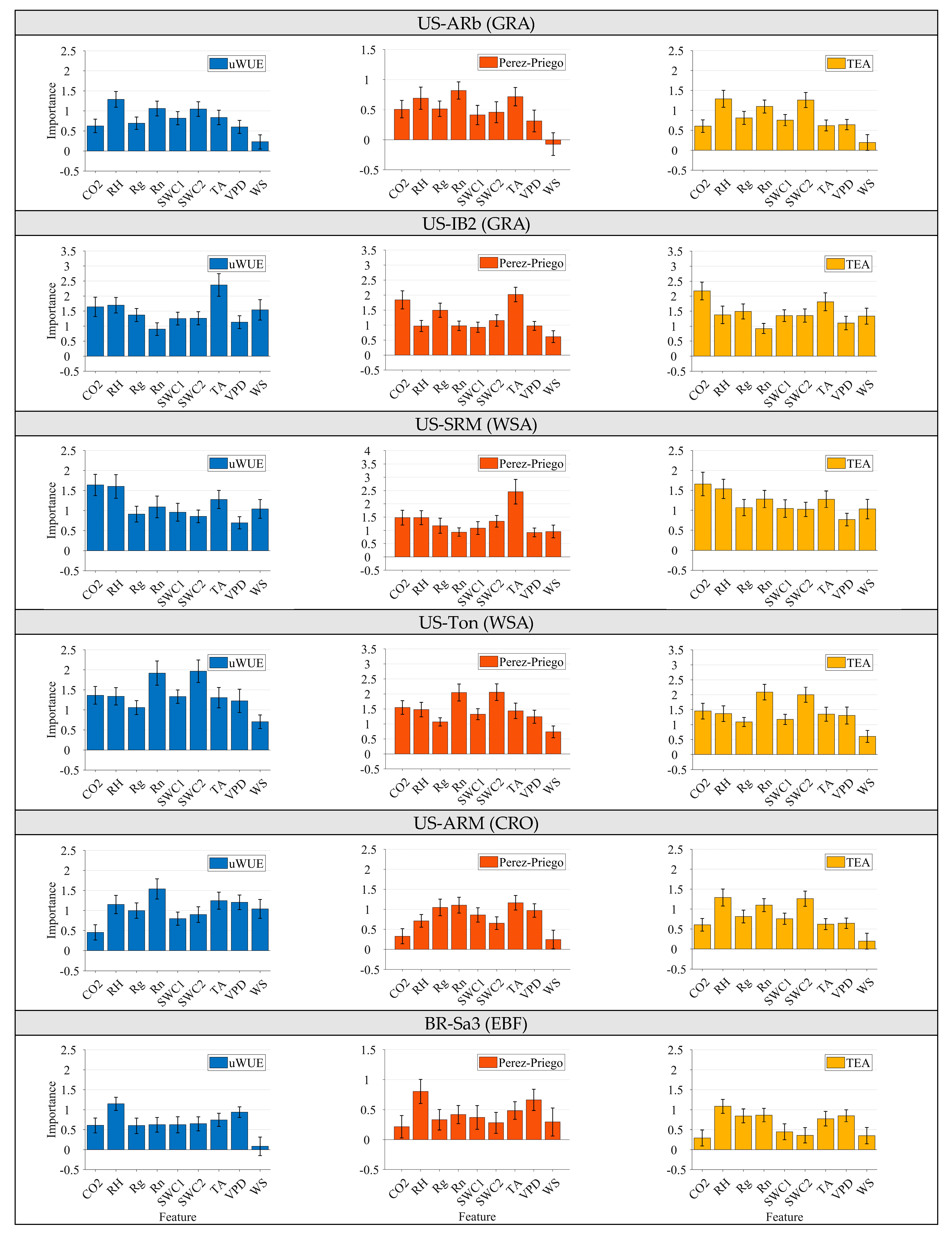
3.1. Differences in Hydrometeorological Effects on G_s in Different Biomes

Hydrometeroglocial effects on G_s were investigated using the method described in Section 2.4.2, and the results are shown in Figure 2. The most important influences on G_s of evergreen broadleaf forests (BR-Sa3 site) were RH, VPD, and TA. For grassland, G_s is more dependent on soil moisture, especially deep-layer soil moisture, as the most important influences on G_s were SWC2 and Rn (US-AR1, US-AR2, and US-ARb site). This dependence on soil moisture is reduced as TA and Rn were the most important influences on G_s in the farmland (US-ARM site), where abundant irrigation could be attributable.

From three sets of daily T estimates, TA, RH, SWC, CO2, and Rn showed high importance in a larger number of cases, which aligns with findings from Zeppel et al. [58], Driesen et al. [31], and Chandra et al. [59], and the WS importance was at the bottom position in most cases. In addition, Rn was also consistently higher in importance than Rg, except for the US-IB2 site and the Perez-Priego method at US-SRM, which is also consistent with the use of Rn rather than Rg in the Penman–Monteith formula [25].

In terms of precipitation, the eight sites can be categorized into four groups: humid (Cfa and Dfa), monsoonal (Am), Mediterranean (Csa and Dsa), and semi-arid (BSk). Among them, the main controller for G_s shows no significant pattern in the humid type (US-ARb, US-ARM, and US-IB2). In contrast, for the Mediterranean type (US-AR1, US-AR2, and US-Ton), the moisture-related environmental factor such as SWC2 ranked higher among factors influencing G_s, and the monsoonal (BR-Sa3) had higher impact of VPD and RH on G_s, while the semi-arid type (US-SRM) had higher RH. This aligns with Kimm et al. [60], who found that in the U.S. Corn Belt’s maize and soybean fields, atmospheric conditions predominantly regulate G_s, underlining the complex interaction between atmospheric moisture demand and soil water availability that dictates plant water use efficiency.

3.2. Consistency of Factors Influencing G_s across Similar Vegetation and Climate

In this study, the results of the importance of characteristics in the same land type were not consistent. Differences develop in the physiological characteristics of plants in different habitats, which gradually disappear when transplanted under the same environmental conditions. Genetically immobilized variation is called ornamental variation, and groups of individuals that differ due to ornamental variation are called ecological phenotypes. The formation of ecotypes is mainly influenced by factors such as climate, soil, and biology. In the classification of ecotypes, the formation of climatic ecotypes is mainly related to climatic conditions and varieties with a wide distribution range from different ecotypes due to differences in climatic conditions in different parts of their distribution areas [61].

US-AR1 and US-AR2 belong to the same Dsa climate and are GRA site types. Rn and SWC2 are ranked higher, while WS and Rg are at the bottom. As a result, there was partial consistency in the G_s influencing factors of the same vegetation between sites under the same climate type. However, hydrothermal and light-temperature conditions in the same climate type were not entirely consistent from year to year, and further categorization based on light-temperature and hydrothermal conditions still needs to be explored. Supporting this, research by Xu et al. [62] indicated inconsistencies in the potential factors affecting stomatal conductance and evapotranspiration at two maize locations under the same climatic conditions, underscoring the complex nature of environmental influences even within defined climatic types.

3.3. Effects of Environmental Elements at Different Vegetation Fertility Stages

Considering that winter wheat ceases growing during the overwintering period [63] and the effects of various elements on its G_s will vary, we delineated mid-December to mid-February of the following year (December 15 of the planting year to February 15 of the following year) as the overwintering period of wheat. We segmented the data from the US-ARM site into the overwintering period and the other growing periods, which were compared with the full-lifecycle results.

Regarding the full-birth and growing periods, TA and Rn are the most contributive factors for G_s in winter wheat, while other factors dominated during the overwintering period (

Table 2. Feature importance of winter wheat growth period and overwintering period.

Period	Method	SWC1	SWC2	VPD	TA	RH	WS	CO2	Rn	Rg
Growing	uWUE	0.8116	1.1922	1.0090	1.1558	1.2629	0.8127	0.4957	1.1381	0.9938
	Perez-Priego	0.9903	0.8785	0.8077	1.2641	0.5956	0.1992	0.4172	1.0697	0.8140
	TEA	1.1261	1.0491	1.2467	1.1335	0.9460	0.8015	0.5262	1.4220	1.0293
Overwintering	uWUE	0.1521	0.2328	0.3372	0.2324	0.2226	0.6757	0.4982	−0.0184	−0.0024
	Perez-Priego	0.3937	0.2208	0.5302	0.5693	0.1855	−0.0222	0.1035	0.0186	0.1759
	TEA	0.2525	0.3437	0.5123	0.5632	0.3119	0.7706	0.3355	0.2498	0.4221

). During the crop growth stage, the transpiration rate was subsequently enhanced with crop growth, and the water-related environmental factors SWC1, SWC2, and VPD showed high importance because water is the basis of crop growth and development, playing the roles of supplying water, transferring nutrients, and forming the structure of important organs. During the overwintering period, the wheat growth is stagnant, the transpiration and net radiation decrease, the temperature drops, and there is less ET [64]. As for the overwintering stage, from the Perez-Priego method with high accuracy (

Table 3. Model accuracy of winter wheat growth period and overwintering period.

Period	Data Set	R2			RMSE (mm/s)
		uWUE	Perez-Priego	TEA	uWUE	Perez-Priego	TEA
Growing	Train	0.7478	0.7691	0.7781	0.4186	0.1503	0.4278
	Test	0.5173	0.6106	0.5738	0.5644	0.2020	0.6077
Overwintering	Train	0.5863	0.6680	0.6397	0.1317	0.0479	0.1832
	Test	0.3114	0.6444	0.3415	0.1708	0.4896	0.2963

), the importance of TA, VPD, and SWC1 remained high, while the importance of SWC2 decreased, and Rn was at the end of the list in all three methods, indicating that the importance of deep soil water content and net radiation on G_s decreased significantly in the growth stagnation and cold stage. Therefore, from the perspective of G_s and crop transpiration during overwintering, the basic physiological needs of the crop should be maintained mainly by controlling the shallow soil water content in the actual production of winter wheat in the field.

3.4. Effect of LAI on Stomatal Conductance Prediction Results

As some of the sites showed slight underfitting, especially BR-Sa3 (Figure 3—Benchmark), this suggests that the model may be relatively simple and fail to effectively learn and capture the complexity and key patterns in the training data. Therefore, more meaningful features need to be added to optimize the model [56,65]. Differences in the main controller of G_s among different growing stages of the same vegetation type demonstrate the different physiological characteristics of plants (Table 2). Studies have shown that stomatal development has a crucial effect on G_s [66], so G_s is highly correlated with the plant growth process. Hence, the importance of the feature varies considerably at different stages of vegetation (Table 2). The classification of vegetation phenological periods is challenging due to variations among plants and the impact of climate change [67]. However, LAI can serve as an indicator of leaf phenology [50]. Moreover, some model studies have attempted to assess the G_s-LAI relationships [68,69]. Therefore, we added LAI to the data samples on a daily scale to see their effect on the accuracy of the results. Since data on the partitioning of ET based on EC differ, the range of values of G_s inversion results obtained from each method is not consistent (generally TEA > uWUE > Perez-Priego), which can affect the RMSE results. The RMSE was only used to compare the differences in the results within the methods. The incorporation of LAI led to enhanced prediction accuracy, as evidenced by the average R² score on training and test data increasing from 0.796 (0.663) to 0.816 (0.799) (Figure 3). Also, LAI consistently ranked highest regarding feature importance (Appendix B, Figure A1). The enhanced accuracy of models incorporating LAI underscores the pivotal role of plant physiological parameters in G_s modeling. This enhancement corroborates the findings of Gaur and Drewry [39], who demonstrated that models integrating physiological predictors (e.g., plant photosynthesis rates) with environmental variables significantly outperformed those that did not. Meanwhile, based on the R² results, the Perez-Priego method exhibited superior performance compared to the other two methods in various biomes, except for evergreen broadleaf forests BR-Sa3. This discrepancy could be attributed to the relatively insignificant variation in LAI across EBF vegetation types or potentially due to the adverse effects of climate impacts on the quality of LAI data [70]. Furthermore, the persistent slight underfitting at certain sites may suggest inherent limitations in the applicability of RF, which requires further in-depth study.

4. Conclusions

This study examined the impact of biophysical factors on G_s across various vegetation types. We observed that the influence of biophysical conditions on G_s varies across different biomes. However, air temperature, relative air humidity, soil water content, and net radiation consistently emerge as significant factors in most cases. In contrast, wind speed consistently exhibits the least influence. Moreover, the effects of environmental factors differ during different stages of vegetation growth. Including LAI enhances the predictive accuracy of G_s, with LAI emerging as the most influential feature. Additionally, when estimating T, the Perez-Priego method generally demonstrates a higher upper limit of prediction accuracy than the other two methods.

There remained some limitations of our work. Firstly, the importance of homogeneous vegetation characteristics among different sites under the same climatic conditions must be further verified. In this study, only US-AR1 and US-AR2 sites, both belonging to Dsa, were selected, and the effects of environmental factors on G_s under homogeneous PFT showed partial consistency but not complete consistency, with some randomness. Meanwhile, even if the climatic conditions are the same, factors such as soil type, water source, production management practices, different species of vegetation, and ecotypes between sites may affect vegetation growth and development, leading to variations in G_s results. Therefore, further research needs to be extended to determine the extent of the influence of these factors. Secondly, while our inclusion of LAI aimed to capture phenological effects on G_s, we acknowledge that the improved model performance may also be attributed to photosynthetic changes preceding LAI variations, indicating the need for further research to disentangle these intertwined mechanisms.

In conclusion, G_s is a critical variable in numerous terrestrial ecohydrology and biophysical models of land surfaces. Our research provides essential guidance on selecting factors for G_s modeling. In practical modeling and applications, one can optimize the selection of feature combinations based on data availability, vegetation type, and climate conditions. This approach enhances the accuracy and efficiency of models, enabling tailored strategies that align with specific environmental scenarios, thereby improving predictions and the management of water and carbon dynamics across diverse ecosystems.

References

1. Hetherington, A.M.; Woodward, F.I. The role of stomata in sensing and driving environmental change. Nature 2003, 424, 901–908. [Google Scholar] [CrossRef] [PubMed]
2. Katul, G.G.; Palmroth, S.; Oren, R. Leaf stomatal responses to vapour pressure deficit under current and CO2-enriched atmosphere explained by the economics of gas exchange. Plant Cell Environ. 2009, 32, 968–979. [Google Scholar] [CrossRef] [PubMed]
3. Sperry, J.S.; Venturas, M.D.; Anderegg, W.R.; Mencuccini, M.; Mackay, D.S.; Wang, Y.; Love, D.M. Predicting stomatal responses to the environment from the optimization of photosynthetic gain and hydraulic cost. Plant Cell Environ. 2017, 40, 816–830. [Google Scholar] [CrossRef] [PubMed]
4. Betts, R.A.; Cox, P.M.; Lee, S.E.; Woodward, F.I. Contrasting physiological and structural vegetation feedbacks in climate change simulations. Nature 1997, 387, 796–799. [Google Scholar] [CrossRef]
5. Betts, R.A.; Boucher, O.; Collins, M.; Cox, P.M.; Falloon, P.D.; Gedney, N.; Hemming, D.L.; Huntingford, C.; Jones, C.D.; Sexton, D.M. Projected increase in continental runoff due to plant responses to increasing carbon dioxide. Nature 2007, 448, 1037–1041. [Google Scholar] [CrossRef] [PubMed]
6. Lemordant, L.; Gentine, P.; Swann, A.S.; Cook, B.I.; Scheff, J. Critical impact of vegetation physiology on the continental hydrologic cycle in response to increasing CO2. Proc. Natl. Acad. Sci. USA 2018, 115, 4093–4098. [Google Scholar] [CrossRef] [PubMed]
7. Wu, Y.; Liu, S.; Abdul-Aziz, O.I. Hydrological effects of the increased CO2 and climate change in the Upper Mississippi River Basin using a modified SWAT. Clim. Chang. 2012, 110, 977–1003. [Google Scholar] [CrossRef]
8. Zhao, J.; Feng, H.; Xu, T.; Xiao, J.; Guerrieri, R.; Liu, S.; Wu, X.; He, X.; He, X. Physiological and environmental control on ecosystem water use efficiency in response to drought across the northern hemisphere. Sci. Total Environ. 2021, 758, 143599. [Google Scholar] [CrossRef] [PubMed]
9. Kannenberg, S.A.; Anderegg, W.R.; Barnes, M.L.; Dannenberg, M.P.; Knapp, A.K. Dominant role of soil moisture in mediating carbon and water fluxes in dryland ecosystems. Nat. Geosci. 2024, 17, 38–43. [Google Scholar] [CrossRef]
10. Mencuccini, M.; Manzoni, S.; Christoffersen, B. Modelling water fluxes in plants: From tissues to biosphere. New Phytol. 2019, 222, 1207–1222. [Google Scholar] [CrossRef]
11. Wu, J.; Serbin, S.P.; Ely, K.S.; Wolfe, B.T.; Dickman, L.T.; Grossiord, C.; Michaletz, S.T.; Collins, A.D.; Detto, M.; McDowell, N.G. The response of stomatal conductance to seasonal drought in tropical forests. Glob. Chang. Biol. 2020, 26, 823–839. [Google Scholar] [CrossRef] [PubMed]
12. Wang, L.; Liu, Z.; Guo, J.; Wang, Y.; Ma, J.; Yu, S.; Yu, P.; Xu, L. Estimate canopy transpiration in larch plantations via the interactions among reference evapotranspiration, leaf area index, and soil moisture. For. Ecol. Manag. 2021, 481, 118749. [Google Scholar] [CrossRef]
13. Du, J.; Dai, X.; Huo, Z.; Wang, X.; Wang, S.; Wang, C.; Zhang, C.; Huang, G. Stand transpiration and canopy conductance dynamics of Populus popularis under varying water availability in an arid area. Sci. Total Environ. 2023, 892, 164397. [Google Scholar] [CrossRef] [PubMed]
14. Stoy, P.C.; El-Madany, T.S.; Fisher, J.B.; Gentine, P.; Gerken, T.; Good, S.P.; Klosterhalfen, A.; Liu, S.; Miralles, D.G.; Perez-Priego, O. Reviews and syntheses: Turning the challenges of partitioning ecosystem evaporation and transpiration into opportunities. Biogeosciences 2019, 16, 3747–3775. [Google Scholar] [CrossRef]
15. Wang, S.; Ibrom, A.; Bauer-Gottwein, P.; Garcia, M. Incorporating diffuse radiation into a light use efficiency and evapotranspiration model: An 11-year study in a high latitude deciduous forest. Agric. For. Meteorol. 2018, 248, 479–493. [Google Scholar] [CrossRef]
16. Celis, J.; Xiao, X.; Basara, J.; Wagle, P.; McCarthy, H. Simple and Innovative Methods to Estimate Gross Primary Production and Transpiration of Crops: A Review. Digit. Ecosyst. Innov. Agric. 2023, 121, 125–156. [Google Scholar]
17. Nelson, J.A.; Pérez-Priego, O.; Zhou, S.; Poyatos, R.; Zhang, Y.; Blanken, P.D.; Gimeno, T.E.; Wohlfahrt, G.; Desai, A.R.; Gioli, B. Ecosystem transpiration and evaporation: Insights from three water flux partitioning methods across FLUXNET sites. Glob. Chang. Biol. 2020, 26, 6916–6930. [Google Scholar] [CrossRef]
18. Zhou, S.; Yu, B.; Zhang, Y.; Huang, Y.; Wang, G. Partitioning evapotranspiration based on the concept of underlying water use efficiency. Water Resour. Res. 2016, 52, 1160–1175. [Google Scholar] [CrossRef]
19. Perez-Priego, O.; Katul, G.; Reichstein, M.; El-Madany, T.S.; Ahrens, B.; Carrara, A.; Scanlon, T.M.; Migliavacca, M. Partitioning eddy covariance water flux components using physiological and micrometeorological approaches. J. Geophys. Res. Biogeosci. 2018, 123, 3353–3370. [Google Scholar] [CrossRef]
20. Nelson, J.A.; Carvalhais, N.; Cuntz, M.; Delpierre, N.; Knauer, J.; Ogée, J.; Migliavacca, M.; Reichstein, M.; Jung, M. Coupling water and carbon fluxes to constrain estimates of transpiration: The TEA algorithm. J. Geophys. Res. Biogeosci. 2018, 123, 3617–3632. [Google Scholar] [CrossRef]
21. Pastorello, G.; Trotta, C.; Canfora, E.; Chu, H.; Christianson, D.; Cheah, Y.-W.; Poindexter, C.; Chen, J.; Elbashandy, A.; Humphrey, M. The FLUXNET2015 dataset and the ONEFlux processing pipeline for eddy covariance data. Sci. Data 2020, 7, 225. [Google Scholar] [CrossRef] [PubMed]
22. Yu, L.; Zhou, S.; Zhao, X.; Gao, X.; Jiang, K.; Zhang, B.; Cheng, L.; Song, X.; Siddique, K.H. Evapotranspiration partitioning based on leaf and ecosystem water use efficiency. Water Resour. Res. 2022, 58, e2021WR030629. [Google Scholar] [CrossRef]
23. Zhou, S.; Yu, B.; Huang, Y.; Wang, G. Daily underlying water use efficiency for AmeriFlux sites. J. Geophys. Res. Biogeosci. 2015, 120, 887–902. [Google Scholar] [CrossRef]
24. Wu, G.; Hu, Z.; Keenan, T.F.; Li, S.; Zhao, W.; Cao, R.C.; Li, Y.; Guo, Q.; Sun, X. Incorporating spatial variations in parameters for improvements of an evapotranspiration model. J. Geophys. Res. Biogeosci. 2020, 125, e2019JG005504. [Google Scholar] [CrossRef]
25. Monteith, J.; Unsworth, M. Principles of Environmental Physics: Plants, Animals, and the Atmosphere; Academic Press: Cambridge, MA, USA, 2013. [Google Scholar]
26. Diefendorf, A.F.; Mueller, K.E.; Wing, S.L.; Koch, P.L.; Freeman, K.H. Global patterns in leaf 13C discrimination and implications for studies of past and future climate. Proc. Natl. Acad. Sci. USA 2010, 107, 5738–5743. [Google Scholar] [CrossRef] [PubMed]
27. Buckley, T.N. How do stomata respond to water status? New Phytol. 2019, 224, 21–36. [Google Scholar] [CrossRef] [PubMed]
28. Ficklin, D.L.; Novick, K.A. Historic and projected changes in vapor pressure deficit suggest a continental-scale drying of the United States atmosphere. J. Geophys. Res. Atmos. 2017, 122, 2061–2079. [Google Scholar] [CrossRef]
29. Urban, J.; Ingwers, M.W.; McGuire, M.A.; Teskey, R.O. Increase in leaf temperature opens stomata and decouples net photosynthesis from stomatal conductance in Pinus taeda and Populus deltoides x nigra. J. Exp. Bot. 2017, 68, 1757–1767. [Google Scholar] [CrossRef] [PubMed]
30. Guo, Z.; Gao, Y.; Yuan, X.; Yuan, M.; Huang, L.; Wang, S.; Liu, C.E.; Duan, C. Effects of heavy metals on stomata in plants: A review. Int. J. Mol. Sci. 2023, 24, 9302. [Google Scholar] [CrossRef]
31. Driesen, E.; Van den Ende, W.; De Proft, M.; Saeys, W. Influence of environmental factors light, CO2, temperature, and relative humidity on stomatal opening and development: A review. Agronomy 2020, 10, 1975. [Google Scholar] [CrossRef]
32. Reichstein, M.; Camps-Valls, G.; Stevens, B.; Jung, M.; Denzler, J.; Carvalhais, N.; Prabhat, F. Deep learning and process understanding for data-driven Earth system science. Nature 2019, 566, 195–204. [Google Scholar] [CrossRef]
33. Sarker, I.H. Machine learning: Algorithms, real-world applications and research directions. SN Comput. Sci. 2021, 2, 160. [Google Scholar] [CrossRef] [PubMed]
34. Hsieh, W.W. Evolution of machine learning in environmental science—A perspective. Environ. Data Sci. 2022, 1, e3. [Google Scholar] [CrossRef]
35. Ellsäßer, F.; Röll, A.; Ahongshangbam, J.; Waite, P.-A.; Schuldt, B.; Hölscher, D. Predicting tree sap flux and stomatal conductance from drone-recorded surface temperatures in a mixed agroforestry system—A machine learning approach. Remote Sens. 2020, 12, 4070. [Google Scholar] [CrossRef]
36. Vitrack-Tamam, S.; Holtzman, L.; Dagan, R.; Levi, S.; Tadmor, Y.; Azizi, T.; Rabinovitz, O.; Naor, A.; Liran, O. Random forest algorithm improves detection of physiological activity embedded within reflectance spectra using stomatal conductance as a test case. Remote Sens. 2020, 12, 2213. [Google Scholar] [CrossRef]
37. Houshmandfar, A.; O’Leary, G.; Fitzgerald, G.J.; Chen, Y.; Tausz-Posch, S.; Benke, K.; Uddin, S.; Tausz, M. Machine learning produces higher prediction accuracy than the Jarvis-type model of climatic control on stomatal conductance in a dryland wheat agro-ecosystem. Agric. For. Meteorol. 2021, 304, 108423. [Google Scholar] [CrossRef]
38. Saunders, A.; Drew, D.M.; Brink, W. Machine learning models perform better than traditional empirical models for stomatal conductance when applied to multiple tree species across different forest biomes. Trees For. People 2021, 6, 100139. [Google Scholar] [CrossRef]
39. Gaur, S.; Drewry, D.T. Explainable machine learning for predicting stomatal conductance across multiple plant functional types. Agric. For. Meteorol. 2024, 350, 109955. [Google Scholar] [CrossRef]
40. Rubel, F.; Kottek, M. Observed and projected climate shifts 1901–2100 depicted by world maps of the Köppen-Geiger climate classification. Meteorol. Z. 2010, 19, 135. [Google Scholar] [CrossRef]
41. Goulden, M. FLUXNET2015 BR-Sa3 Santarem-Km83-Logged Forest; FluxNet; University of California-Irvine: Irvine, CA, USA, 2016. [Google Scholar]
42. Billesbach, D.; Bradford, J.; Torn, M. FLUXNET2015 US-AR1 ARM USDA UNL OSU Woodward Switchgrass 1; FluxNet; Lawerence Berkeley National Lab, US Department of Agriculture (USDA): Berkeley, CA, USA, 2016. [Google Scholar]
43. Billesbach, D.; Bradford, J.; Torn, M. AmeriFlux FLUXNET-1F US-AR2 ARM USDA UNL OSU Woodward Switchgrass 2; Lawrence Berkeley National Laboratory (LBNL): Berkeley, CA, USA, 2023. [Google Scholar]
44. Torn, M. FLUXNET2015 US-ARb ARM Southern Great Plains Burn Site-Lamont; FluxNet; Lawrence Berkeley National Lab. (LBNL): Berkeley, CA, USA, 2016. [Google Scholar]
45. Biraud, S.; Fischer, M.; Chan, S.; Torn, M. AmeriFlux FLUXNET-1F US-ARM ARM Southern Great Plains Site-Lamont; AmeriFlux; Lawrence Berkeley National Lab. (LBNL): Berkeley, CA, USA, 2022. [Google Scholar]
46. Matamala, R. FLUXNET2015 US-IB2 Fermi National Accelerator Laboratory-Batavia (Prairie Site); FluxNet; Argonne National Lab. (ANL): Argonne, IL, USA, 2016. [Google Scholar]
47. Scott, R. AmeriFlux AmeriFlux US-SRM Santa Rita Mesquite; Lawrence Berkeley National Laboratory (LBNL): Berkeley, CA, USA, 2016. [Google Scholar]
48. Ma, S.; Xu, L.; Verfaillie, J.; Baldocchi, D. AmeriFlux FLUXNET-1F US-Ton Tonzi Ranch; Lawrence Berkeley National Laboratory (LBNL): Berkeley, CA, USA, 2023. [Google Scholar]
49. Zhang, K.; Zhu, G.; Ma, J.; Yang, Y.; Shang, S.; Gu, C. Parameter analysis and estimates for the MODIS evapotranspiration algorithm and multiscale verification. Water Resour. Res. 2019, 55, 2211–2231. [Google Scholar] [CrossRef]
50. Jin, J.; Yan, T.; Wang, H.; Ma, X.; He, M.; Wang, Y.; Wang, W.; Guo, F.; Cai, Y.; Zhu, Q. Improved modeling of canopy transpiration for temperate forests by incorporating a LAI-based dynamic parametrization scheme of stomatal slope. Agric. For. Meteorol. 2022, 326, 109157. [Google Scholar] [CrossRef]
51. BADM: Biological, Ancillary, Disturbance, and Metadata. Available online: https://ameriflux.lbl.gov/data/badm/ (accessed on 16 April 2024).
52. Nelson, J. Jnelson18/Ecosystem-Transpiration: Additional Installation Instructions (v1.1). 2020. Available online: https://zenodo.org/records/3921923 (accessed on 1 January 2023). [CrossRef]
53. Smith, M.; Allen, R.; Periera, L.; Raes, D. Crop Evapotranspiration: Guidelines for Computing Crop Water Requirements; FAO Irrigation and Drainage Paper 56; FAO: Rome, Italy, 1998. [Google Scholar]
54. Myneni, R.; Knyazikhin, Y.; Park, T. MODIS/Terra+Aqua Leaf Area Index/FPAR 4-Day L4 Global 500m SIN Grid V061; USGS: Sioux Falls, SD, USA, 2021. [CrossRef]
55. Croft, H.; Chen, J.M.; Luo, X.; Bartlett, P.; Chen, B.; Staebler, R.M. Leaf chlorophyll content as a proxy for leaf photosynthetic capacity. Glob. Chang. Biol. 2017, 23, 3513–3524. [Google Scholar] [CrossRef] [PubMed]
56. Hastie, T.; Tibshirani, R.; Friedman, J.H.; Friedman, J.H. The Elements of Statistical Learning: Data Mining, Inference, and Prediction, 2nd ed.; Springer: New York, NY, USA, 2009. [Google Scholar]
57. Zhu, R.; Zeng, D.; Kosorok, M.R. Reinforcement learning trees. J. Am. Stat. Assoc. 2015, 110, 1770–1784. [Google Scholar] [CrossRef] [PubMed]
58. Zeppel, M.J.; Lewis, J.D.; Chaszar, B.; Smith, R.A.; Medlyn, B.E.; Huxman, T.E.; Tissue, D.T. Nocturnal stomatal conductance responses to rising [CO2], temperature and drought. New Phytol. 2012, 193, 929–938. [Google Scholar] [CrossRef] [PubMed]
59. Chandra, S.P.; Adiga, V.; Chinmaya, P.; Kikkeri, V.V.; Senapati, S. Modulation of stomatal conductance in response to changes in external factors for plants grown in the tropical climate. J. High Sch. Sci. 2023, 7, 1–17. [Google Scholar]
60. Kimm, H.; Guan, K.; Gentine, P.; Wu, J.; Bernacchi, C.J.; Sulman, B.N.; Griffis, T.J.; Lin, C. Redefining droughts for the US Corn Belt: The dominant role of atmospheric vapor pressure deficit over soil moisture in regulating stomatal behavior of Maize and Soybean. Agric. For. Meteorol. 2020, 287, 107930. [Google Scholar] [CrossRef]
61. Rana, M.S.; Rath, J.R.; Reddy, C.V.; Pelzang, S.; Shelke, R.G.; Patel, S. Ecotypic adaptation of plants and the role of microbiota in ameliorating the environmental extremes using contemporary approaches. In Rhizobiome; Elsevier: Amsterdam, The Netherlands, 2023; pp. 377–402. [Google Scholar]
62. Xu, J.; Wu, B.; Ryu, D.; Yan, N.; Zhu, W.; Ma, Z. Quantifying the contribution of biophysical and environmental factors in uncertainty of modeling canopy conductance. J. Hydrol. 2021, 592, 125612. [Google Scholar] [CrossRef]
63. Hao, Z.; Geng, X.; Wang, F.; Zheng, J. Impacts of climate change on agrometeorological indices at winter wheat overwintering stage in Northern China during 2021–2050. Int. J. Climatol. 2018, 38, 5576–5588. [Google Scholar] [CrossRef]
64. Feng, X.; Liu, H.; Feng, D.; Tang, X.; Li, L.; Chang, J.; Tanny, J.; Liu, R. Quantifying winter wheat evapotranspiration and crop coefficients under sprinkler irrigation using eddy covariance technology in the North China Plain. Agric. Water Manag. 2023, 277, 108131. [Google Scholar] [CrossRef]
65. Bishop, C. Pattern Recognition and Machine Learning; Springer: New York, NY, USA, 2006. [Google Scholar]
66. Wu, B.-J.; Chow, W.S.; Liu, Y.-J.; Shi, L.; Jiang, C.-D. Effects of stomatal development on stomatal conductance and on stomatal limitation of photosynthesis in Syringa oblata and Euonymus japonicus Thunb. Plant Sci. 2014, 229, 23–31. [Google Scholar] [CrossRef] [PubMed]
67. Wu, L.; Ma, X.; Dou, X.; Zhu, J.; Zhao, C. Impacts of climate change on vegetation phenology and net primary productivity in arid Central Asia. Sci. Total Environ. 2021, 796, 149055. [Google Scholar] [CrossRef] [PubMed]
68. Launiainen, S.; Katul, G.G.; Kolari, P.; Lindroth, A.; Lohila, A.; Aurela, M.; Varlagin, A.; Grelle, A.; Vesala, T. Do the energy fluxes and surface conductance of boreal coniferous forests in Europe scale with leaf area? Glob. Chang. Biol. 2016, 22, 4096–4113. [Google Scholar] [CrossRef] [PubMed]
69. Roberts, J. Forest transpiration: A conservative hydrological process? J. Hydrol. 1983, 66, 133–141. [Google Scholar] [CrossRef]
70. Fang, H.; Wei, S.; Jiang, C. Intercomparison and uncertainty analysis of global MODIS, cyclopes, and GLOBCARBON LAI products. In Proceedings of the 2012 IEEE International Geoscience and Remote Sensing Symposium, Munich, Germany, 22–27 July 2012; pp. 5959–5962. [Google Scholar]
Figure 1. Locations of the study sites.
Water 16 02251 g001
Figure 2. Histogram of the importance of Gs characteristics at each site. The y-axis starts at −0.5 because the importance and error bars exceed 0 for some sites, and the negative y indicates that the feature hurts the RF prediction results.
Water 16 02251 g002aWater 16 02251 g002b
Figure 3. Model accuracy of before (Benchmark) and after adding LAI (LAI). The darker colors in the panels correspond to higher values. (a) presents R2 results for the training set, while (b) displays R2 results for the test set. (c) shows RMSE outcomes for the training set, and (d) outlines RMSE results for the test set.
Water 16 02251 g003