Using Machine Learning Models for Short-Term Prediction of Dissolved Oxygen in a Microtidal Estuary

Abstract

This paper presents a comprehensive approach to predicting short-term (for the upcoming 2 weeks) changes in estuarine dissolved oxygen concentrations via machine learning models that integrate historical water sampling, historical and upcoming 2-week meteorological data, and river discharge and discharge metrics. Dissolved oxygen is a critical indicator of ecosystem health, and this approach is implemented for the Neuse River Estuary, North Carolina, U.S.A., which has a long history of hypoxia-related habitat degradation. Through meticulous data preprocessing and feature selection, this research evaluates the predictions of dissolved oxygen concentrations by comparing a recurrent neural network with four other models, including a Multilayer Perceptron, Long Short-Term Memory, Gradient Boosting, and AutoKeras, through sensitivity experiments. The input predictors to our prediction models include water temperature, turbidity, chlorophyll-a, aggregated river discharge, and aggregated wind based on eight directions. By emphasizing the most impactful predictors, we streamlined the model-building processes and built a hindcast system from 2015 to 2019. We found that the recurrent neural network model was most effective in predicting the dissolved oxygen concentrations, with an R² value of 0.99 at multiple stations. Different from our machine learning hindcast models that used observed upcoming meteorological and discharge data, an actual forecast system would use forecasted meteorological and discharge data. Therefore, an actual operational forecast may have lower accuracy than the hindcast, as determined by the accuracy of the predicted meteorological and discharge data. Nevertheless, our studies enhance our understanding of the factors influencing dissolved oxygen variability and set the basis for the implementation of a predictive tool for environmental monitoring and management. We also emphasized the importance of building station-specific models to improve the prediction results.

1. Introduction

The escalating threat to ocean water quality places strain on essential marine water resources, fishery habitats, and ecosystems [1,2,3]. As one of the most important indicators of water quality, dissolved oxygen (DO) shows the amount of oxygen that is available to fish, invertebrates, and organisms in the water. The DO concentration must be above certain levels to support aquatic life and assure the stability of the aquatic ecosystem. Low levels of oxygen (hypoxia) occur when thermal/haline stratification is strong, coupled with excessive algae growth and depletion of DO as the algae die, sink, and decompose. A common definition of hypoxia is DO < 2 mg/L, while others have thresholds ranging from 1 to 6 mg/L [4,5,6].

Forecasting DO concentrations can enhance ecosystem restoration and safeguard vital ecosystem services by providing advanced warnings of events that could cause water quality changes, as well as offering advanced information for field observations. Due to the intricate hydrodynamical and biogeochemical processes in estuarine and coastal waters, it is challenging to accurately predict DO [7]. Various methods, including mechanistic, statistical, and hybrid models, have been employed to predict DO [8,9,10]. The mechanistic models are based on biogeochemical processes, including plankton dynamics, nutrient cycling, air/sea interactions, and benthic processes [11,12,13]. They often rely on lab studies or empirical observations, leading to potential errors, especially when coupled with intricate hydrodynamic models. Another evident drawback of these models is the significant computational time consumption and associated costs. Statistical models are also adopted by researchers [10,14,15]. However, their foundational assumptions may not adequately address critical complex patterns, with discrepancies arising from the oversimplified relationships between various factors.

Machine learning is a promising approach due to its impressive performance in capturing the impacts of non-linear processes for engineering systems [3,16,17]. In recent years, researchers have buttressed DO predictions in coastal ecosystems by employing a range of machine learning models, like artificial neural networks (ANNs) [18], linear regression (LR) [19], and Support Vector Machines (SVMs) [20,21,22,23]. Among them, the ANN models are adaptable mathematical structures that can recognize intricate non-linear relationships or patterns between input and output information. Additionally, ANNs may estimate the output values by utilizing training and learning processes [24].

A type of ANN known as a recurrent neural network (RNN) was recently shown to be more effective than other neural network designs in modeling sequence data, such as time series or natural language [25]. In 2022, Nair and Vijaya [26] evaluated the effectiveness of RNNs and Long Short-Term Memory (LSTM) with a range of conventional machine learning techniques, including random forest, linear regression, Multi-Layer Perceptron (MLP) regression, and support vector regression, in predicting DO concentrations. Their models were developed and verified utilizing data on river water quality that were gathered from 11 stations between 2016 and 2020. The outcomes demonstrated that, in comparison to other algorithms, the RNN model had the best prediction accuracy for DO.

In this paper, we aim to enhance the accuracy of short-term DO concentration prediction in predicting the DO in the upcoming two weeks based on upcoming and historical observations, using the Neuse River Estuary (NRE) in North Carolina, USA, as our example. It will be the first machine-learning-model-based short-term DO forecast system for the NRE system. We comprehensively compare the RNN’s performance in bottom water DO prediction at 11 sampling stations with alternative models, including Gradient Boosting (GB) [27], LSTM networks [28], MLP [29], and AutoKeras [30]. We experimented with diverse combinations of input features extracted from related datasets, including the NRE Modeling and Monitoring program (ModMon [1]) dataset, river discharge data, and NOAA NDBC meteorological data, to develop machine learning models. The system developed in the study is examined using hindcast simulations, which utilize observed upcoming input features to constrain the uncertainties caused by predicted upcoming meteorological and river data. In a real-time operational forecast, model-predicted upcoming meteorological and river data would be used.

This research delves into the intricate dynamics of the NRE, offering insights into DO variations and the factors influencing water quality. In Section 3, we offer a comprehensive explanation of the datasets and data processing methods used and outline the models we applied to DO prediction. The model results are shown in Section 4, followed by discussions about future directions and suggestions for further work in Section 5.

2. Materials and Methods

2.1. Study Area and Data

The NRE is formed by the Neuse River (Figure 1), which drains North Carolina’s fourth largest basin, including rapidly urbanizing areas in the Piedmont around Raleigh and Durham and intensive row crop and swine and poultry agriculture on the coastal plain. The NRE is a drowned river valley that spans approximately 70 km, with an average depth of 3.5 m, and is a critical habitat for fisheries and wildlife. Sustainable management of the NRE–Pamlico Sound coastal ecosystems is crucial for both the environment and local economies [31,32]. Hypoxia, a challenge confronting the NRE, is exacerbated by increased terrestrial nutrient flux from the conversion of forests into agricultural and urban landscapes and a rise in wastewater discharge [33,34]. It directly impacts vital fishery habitats and recreational areas, highlighting the need for accurate water quality predictions for stakeholders, including fishery managers, anglers, and water resource authorities [35].

To address water quality problems, the ModMon program has monitored DO, chlorophyll-a (Chl-a), and other biogeochemical and ecological parameters at 11 mid-river sampling stations along the NRE from the river head to its mouth at Pamlico Sound since 1994. The program conducts nearly bi-weekly sampling of hydrographic, chemical, and ecological parameters from surface (0.2 m depth) and bottom (0.5 m above bottom) depths throughout the year [1]. Extensive and comprehensive datasets lay the groundwork for machine learning models.

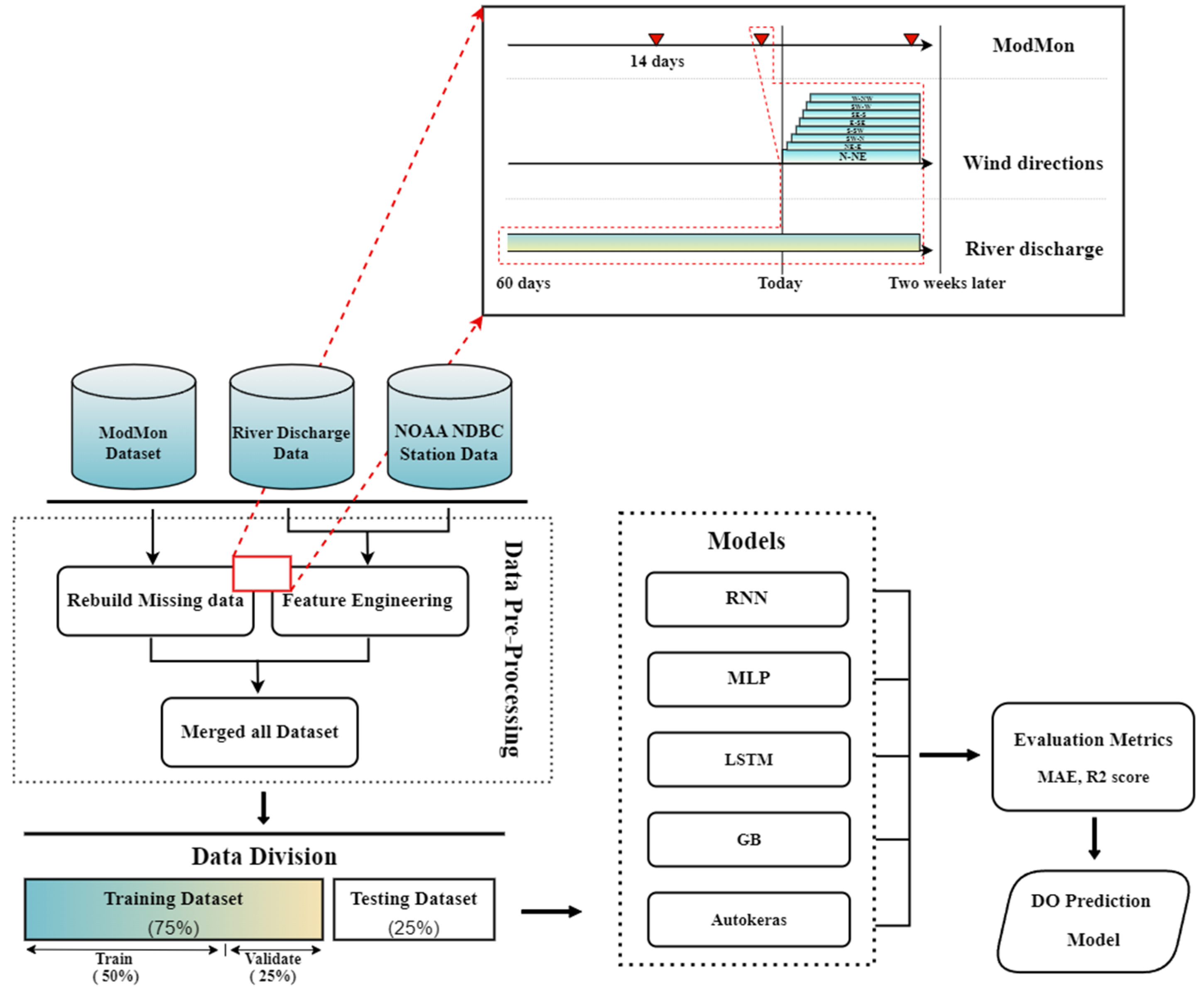
Figure 2 provides an overview of our approach to predicting the DO concentrations using different machine learning models, including the RNN, GB, LSTM, MLP, and AutoKeras. In the diagram, “Today” represents the model initialization time, and the machine learning models predict the DO concentration 14 days later (the 14th day after model initialization is called the prediction time thereafter), with input features including ModMon sampling at a time before and closest to the model initialization time, the 14-day wind data before the prediction time, and the 60-day river discharge data before the prediction time.

We start by collecting datasets from diverse sources, including the ModMon dataset and river discharge and meteorological data. The ModMon dataset includes nearly bi-weekly samples for 14 variables—water temperature, turbidity, chlorophyll-a (Chl-a), particulate organic carbon (POC), particulate nitrogen (PN), carbon-to-nitrogen ratio (CtoN), nitrate/nitrite (NO₃/NO₂), dissolved inorganic nitrogen (DIN), total dissolved nitrogen (TDN), dissolved organic nitrogen (DON), orthophosphate (PO₄), silica (SiO₂), ammonium (NH₄), and DO—for 11 NRE stations (stations 0, 20, 30, 50, 60, 70, 100, 120, 140, 160, and 180; Figure 1) from 2000 to 2017. Data on the daily river discharge from the Neuse River are accessed from the U.S. Geological Survey (USGS) site 02091814 (https://waterdata.usgs.gov/nwis/; accessed on 1 January 2023). Hourly meteorological data, including wind speed and direction, air pressure, and air temperature, were obtained from the NOAA NDBC station near Cape Lookout Bight, NC (station CLKN7; https://www.ndbc.noaa.gov; accessed on 1 January 2023).

In the first phase of our workflow, we merged the datasets into a cohesive data structure with a temporal resolution of 2 weeks and filled in missing data by linear interpolation for continuity.

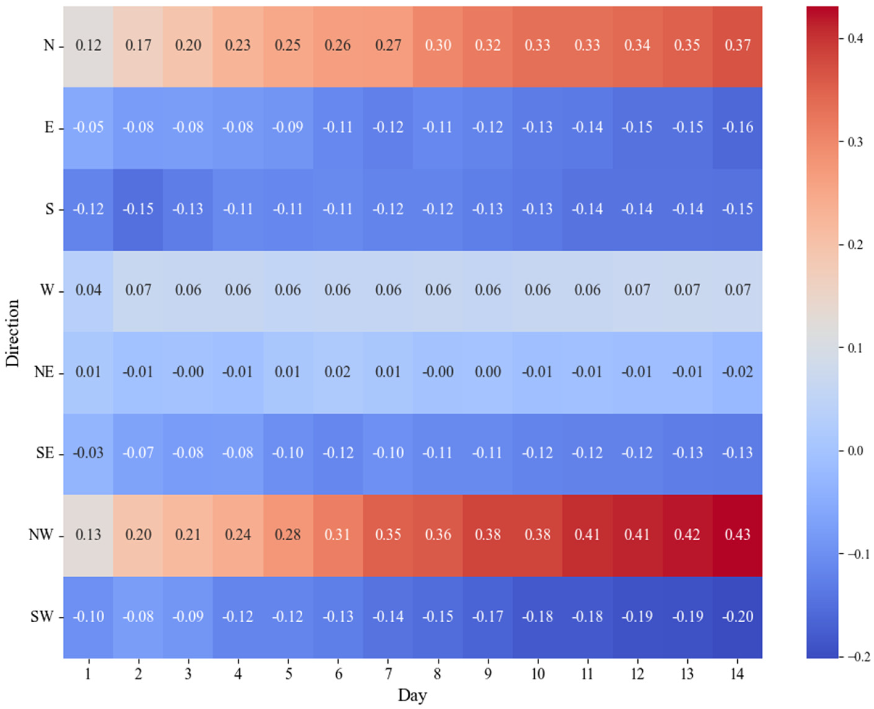
In addition to the original 14 variables in the ModMon dataset, we included the manipulated wind and river discharge as input features and used feature selection to identify the most important predictors. Considering the importance of the wind direction and the wind’s accumulative effect in modulating physical and ecological processes, we included the aggregated (summed) wind speeds over 1- to 14-day periods before the prediction time in eight directional sectors (N-NE, NE-E, E-SE, SE-S, S-SW, SW-W, W-NW, and NW-N) as input features. Then, we analyzed the correlation between the aggregated wind data in the directional sectors and the DO concentrations (Figure 3) and identified the top three combinations that had the strongest correlation with DO, namely aggregated NW-N wind over 14 days (NW14), N-NE wind over 14 days (N14), and SW-W wind over 14 days (SW14), with correlation coefficients of 0.43, 0.37, and −0.20, respectively.

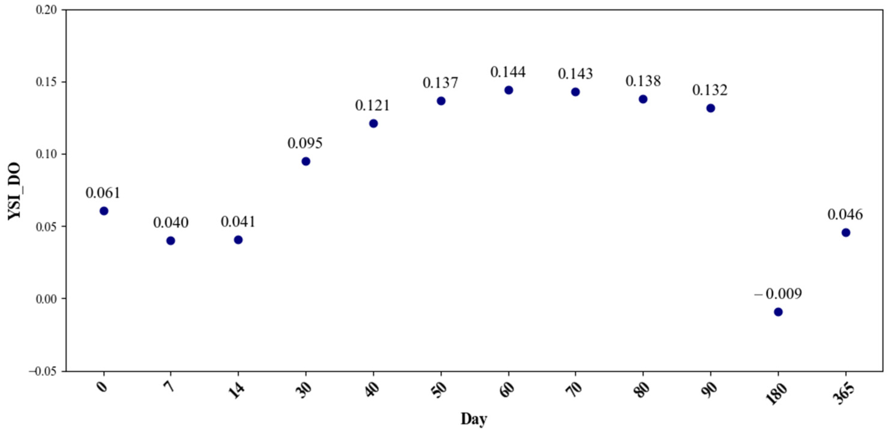
To examine the time-delayed and accumulative effects from the upstream river, we summed the Neuse River discharge from a week to a year preceding the prediction time (named ACC_Flow below). We found that some aggregations of discharge data had notable correlations with the DO concentrations, particularly over the 60 days before the prediction time, with a correlation coefficient of 0.144, as Figure 4 depicts.

Therefore, besides the 14 variables in the ModMon dataset, we included NW14, SW14, N14, ACC_Flow, and Atmospheric Temperature (ATMP) as additional input features. In the first phase of our workflow, we merged all the input features into a cohesive data structure with a temporal resolution of 2 weeks and filled in missing data by linear interpolation and lasso imputation, with gaps of missing data smaller than a week. In instances of extended data absences longer than one week, records from a nearby station operated by the United States Coast Guard and Department of Homeland Security NDBC station 41025 (LLNR 637, Diamond Shoals, NC; https://www.ndbc.noaa.gov/; accessed on 1 January 2023) were used to substitute the missing entries. Resampling the data at bi-weekly intervals completes the preprocessing, synchronizing the dataset with the LSTM model’s temporal requirements. Such rigorous preprocessing not only underpins the models’ robustness but also improves their predictive accuracy for hypoxic conditions in the NRE.

The initial merging of all the datasets with ModMon data using a left join preserved crucial observations. Segmentation by station resulted in 11 distinct data subsets used for model training and testing.

2.2. Machine Learning Models

We employed diverse models to predict the DO concentrations, including RNN, LSTM, GB, MLP, and AutoKeras as a representative of automated machine learning (AutoML) techniques. Each model was chosen for its unique ability to capture and learn from temporal and non-linear patterns within the data.

To evaluate the accuracy and variance explained by each model, we used two standard evaluation metrics, the Mean Absolute Error (MAE) and the R-squared (R²) score, with smaller MAE and greater R-squared values indicating better performance. These metrics offer insight into the accuracy and the variance explained by the models, respectively.

In addition, we included an evaluation metric for binary event forecasts to assess our models’ performance in predicting the occurrence of hypoxia (using a threshold value of 2 mg/L)—the Peirce Skill Score (PSS)—which is defined as

$$PSS=\frac{\left(ad-bc\right)}{\left(b+d\right)\left(a+c\right)}$$

where $a$ represents the number of correctly predicted occurrences of hypoxia (hits); $b$ incorrectly predicted hypoxia (false alarms); $c$ false negatives (misses); and $d$ correctly predicted absences of hypoxia [35,36]. The PSS is in the range of [–1, 1], with larger values representing a better performance.

2.2.1. The Multi-Layer Perceptron (MLP)

The MLP stands out as a widely embraced and extensively utilized neural network model, playing a pivotal role in the contemporary era of big data analytics [37]. The MLP is composed of three distinctive types of layers: the input layer, which accepts the input dataset; the hidden layers, where feature processing takes place; and the output layer that provides the predicted results. In this architecture, the input signal is passed through layer by layer [38,39]. This network serves as the core model for our DO forecasting efforts.

In our MLP model, we utilized one input layer, two hidden layers, and one output layer for the regression predictions. In the context of an MLP model, the input vector X includes individual features, $x_1,x_2,\dots ,x_n$. Each feature is associated with a weight ($w$) that signifies its importance, and a bias (b) term is added. The computations for a single neuron in the layer are expressed as

$$Z=x_1.w_1+x_2.w_2+\dots +x_n.w_n+b$$

The result (Z) is then passed through an activation function to introduce non-linearity, expressed as

$$y=Activation \left(z\right)$$

This process is repeated through each layer, with the output of one layer serving as the input for the next, until the final output layer is reached.

2.2.2. The Recurrent Neural Network (RNN)

The RNN is one of the ANN structures known to be effective in extracting patterns from sequence data, including time series or natural language. This model demonstrates remarkable characteristics, such as a strong prediction performance and the ability to capture long-term temporal correlations in observations with variable lengths [40,41]. The RNN sequentially runs the relationships between nodes in a direct cycle graph, allowing temporal dynamic behavior to be identified. It is effective in multiple domains because it can handle temporal sequences and store sequence information from previous inputs in internal memory by offering a recurrent hidden state that recognizes relationships across time scales [26].

Following partitioning the dataset into two parts based on the experimental setup, we implemented an RNN model with multiple layers. Each layer possesses its unique set of biases and weights. This model enables the recognition of temporal dynamic behavior by sequentially evaluating the connections between nodes within a cyclic graph structure [26]. In our RNN model, as shown in Figure 5, each input sequence $x_1,x_2,\dots ,x_n$ undergoes dynamic transformation through two SimpleRNN layers, incorporating weights ($w_{in},w_{hidden},w_{out}$) and biases ($b_{in},b_{hidden},b_{out}$). The first layer generates a hidden layer ($A_{in}$), subject to dropout for regularization, while the second layer refines these states using ReLU activation. The final output ($Y_{pre}$) results from applying weights and biases to the refined hidden layers. This sequential process captures intricate temporal dependencies, which is crucial for accurate predictions. The RNN computation is summarized as

$$Y_{pre}=Activation \left(A_{in}^{\prime }.w_{hidden}+b_{hidden}\right).w_{out}+b_{out}$$

in which $A_{in}^{\prime }$ represents the dropout-modified hidden layers from the first layer, and $Activation$ denotes the ReLU activation function. Figure 5 illustrates the structure of the RNN.

2.2.3. Long Short-Term Memory (LSTM) Networks

An LSTM neural network represents an advancement over the traditional RNNs by effectively addressing the RNN’s memory attenuation issue [25,42]. LSTM has been applied for predictive purposes, encompassing the estimation of total phosphorus and DO and the forecasting of temporal water quality, including Chl-a concentration [35]. We intended to utilize LSTM for DO prediction. An LSTM layer consists of a series of interconnected blocks, each of which incorporates memory cells designed to store and transmit sequential information. Each LSTM memory cell features three crucial information gates, the input gate, the forget gate, and the output gate, as well as two distinct states, the cell state and the hidden state. These components collectively manage what to retain, what to discard, and what to remember across time steps, enabling the network to learn and model long-term dependencies [7].

2.2.4. Gradient Boosting (GB)

The GB machine learning algorithm operates as an additive model, where each subsequent model in the ensemble is designed to correct and enhance the performance of the preceding ones. Unlike traditional models that build upon one another sequentially, GB employs a unique feed-forward approach [43,44]. It minimizes the errors made by earlier models by placing greater emphasis on the instances where they fall short, resulting in a powerful ensemble that excels in its predictive accuracy. GB’s strength lies in its ability to sequentially refine predictions, making it particularly effective for complex and non-linear relationships within data. By iteratively improving upon the weaknesses of earlier models, GB has become a popular and powerful technique in machine learning.

2.2.5. AutoKeras

Compared with statistical models, neural network models can effectively model the complex non-linearities between input features and predictors. However, selecting the optimal models/hyperparameters/neural network structure requires extensive searches. One of the primary goals of the AutoML approaches is to automate the process of selecting and tuning ML models, bridging the knowledge gap between domain experts (such as marine scientists) and computational scientists. AutoKeras, a Python-based open-source tool, empowers users to apply AutoML to deep learning models using Keras’ application programming interface (API). AutoKeras stands out as an efficient and user-friendly tool for automatically discovering high-performing models across a diverse spectrum of forecasting tasks, including regression datasets and structured data, such as tabular formats [45].

2.3. The Model Application Process

With our datasets prepared, we partitioned the data into a training set, constituting 75% of the total from 2000 to 2015, and a test set, comprising the remaining 25% from 2015 to 2019 [16] (Figure 2). This split ensured both the thorough training of our models and a rigorous evaluation of their predictive performance.

As part of the iterative training process, some models, such as the RNN, took part of the training samples as validation; in this case, the validation dataset came from the training dataset. The validation dataset served to assess the models’ performance on unseen data, aiding in the evaluation of their accuracy and generalization to new information.

Based on the segmentation of the stations, we obtained 11 distinct data subsets comprising both past and present DO values. Each model was trained independently for each station after the data segmentation. Considering the difference in the water depth, geometry, and distance to the river mouth and the coastal ocean, the different stations will respond differently to the same environmental factors. The risk of low DO/hypoxia differs by station. For instance, the RNN model for station 0 was trained independently compared to station 10, so those two models had different parameters despite both models utilizing the same RNN structure. By training the models independently for each station, we can enhance the effectiveness and adaptability of the models.

2.4. Model Parameter Tuning

A crucial step involved in achieving optimal performance in our machine learning models was fine-tuning their hyperparameters.

Table 1. The parameters of RNN, MLP, LSTM, GB, and AutoKeras models.

Models	Parameters	Value	Models	Parameters	Value
RNN	Learning rate	0.001	LSTM	Learning rate	0.001
	Loss	Mean squared error		Loss	Mean squared error
	Epochs	200		Epochs	200
	Batch size	32		Batch size	32
	The units of the RNN	100		The units of the LSTM	100
MLP	Learning rate	0.001	GB	Learning rate	0.1
	Loss	Mean squared error		Number of estimators	100
	Epochs	300		Random state	32
	Batch size	32	AutoKeras	Epochs	300
	The units of the MLP	128, 64 and 32		The units of AutoKeras	32, 32, 32, and 1

presents an overview of the tuned parameters for each model in our experiments, namely the RNN, LSTM, the MLP, GB, and the automated machine learning approach facilitated by AutoKeras. Both the RNN and LSTM, sophisticated models capable of processing sequential data, were tuned with a consistent learning rate of 0.001. This ensured steady convergence during training while minimizing the mean squared error, our chosen loss function. The batch size was set to 32 across these models, with the epoch count for training fixed at 200 [17]. A total of 100 units were chosen for the hidden layers, striking a balance between the models’ ability to learn complex patterns and their computational tractability.

The MLP, a dense network model, was parameterized with varied layer units of 128, 64, and 32 to provide a hierarchical feature extraction mechanism. A longer training period of 300 epochs was set for this model [2], with other parameters such as the learning rate and batch size mirroring those of the RNN and LSTM models. Conversely, the GB model, a robust ensemble technique, utilized a higher learning rate of 0.1 to foster faster convergence, while the number of estimators was set as 100 to build a strong learning model. The random state was held constant at 32 to ensure the reproducibility of the results. This model also underwent a 300-epoch training regimen.

AutoKeras was programmed with a distinct configuration of 32 units for the first three layers and one unit for the output layer. AutoKeras optimizes its architecture internally, allowing us to streamline the model selection process. The hyperparameter values detailed in Table 1 were determined through an iterative process of experimentation, considering both the performance on the validation set and the computational resources at our disposal. The subsequent sections will elaborate on how the fine-tuning of these parameters significantly influenced the models’ prediction accuracies and learning capabilities.

3. Results

We compared the five models’ performance in DO prediction in

Table 2. Performance comparison of the five models for DO concentration prediction.

Station		0	20	30	50	60	70	100	120	140	160	180
RNN	MAE	0.13	0.17	0.18	0.13	0.14	0.16	0.12	0.16	0.14	0.11	0.11
	R2	0.99	0.99	0.99	0.99	0.99	0.99	0.99	0.99	0.99	0.99	0.99
	PSS	1.00	1.00	0.96	1.00	0.90	1.00	0.94	0.90	1.00	0.97	0.99
MLP	MAE	0.24	0.31	1.43	0.29	0.48	0.52	0.51	0.41	0.54	0.46	0.31
	R2	0.98	0.98	0.77	0.98	0.96	0.96	0.95	0.96	0.94	0.96	0.96
	PSS	1.00	0.88	0.85	0.93	0.83	0.68	0.92	0.40	0.86	0.49	0.00
LSTM	MAE	0.24	0.24	0.46	0.29	0.45	0.53	0.30	0.45	0.28	0.29	0.31
	R2	0.98	0.98	0.96	0.98	0.96	0.95	0.98	0.96	0.98	0.98	0.96
	PSS	0.00	0.87	0.86	0.96	0.83	0.85	0.74	0.88	0.99	0.85	0.00
GB	MAE	0.15	0.19	0.28	0.28	0.31	0.32	0.29	0.26	0.19	0.23	0.21
	R2	0.99	0.99	0.98	0.98	0.98	0.98	0.98	0.98	0.99	0.98	0.98
	PSS	1.00	0.88	0.93	0.98	0.79	0.86	0.94	0.82	0.75	0.90	1.00
AutoKeras	MAE	0.39	0.93	0.26	0.32	1.45	0.93	0.41	0.50	0.38	0.12	0.39
	R2	0.93	0.82	0.98	0.98	0.69	0.90	0.97	0.95	0.96	0.99	0.96
	PSS	0.00	0.94	0.57	0.84	0.61	1.00	0.97	0.98	0.99	0.87	1.00

and Figure 6 and Figure 7, with Table 2 showing the metrics of MAE, R², and the PSS. As indicated in Table 2, the RNN and GB models exhibited superior performance, maintaining low MAE values (<0.32) and high R² values across all tested sites. Notably, the RNN model achieved an R² value of 0.99 at multiple sites, suggesting an solid predictive capability within the constraints of the experiment. The PSS scores for the RNN models range from 0.90 to 1.00, and for the GB models, they range from 0.75 to 1, demonstrating great performance in predicting the occurrence of hypoxia. On the other hand, the AutoKeras models showed significant variability in their MAE (ranging from 0.12 to 1.45) and R² values (ranging from 0.69 to 0.99), implying a less consistent predictive performance. The PSS scores for AutoKeras range from 0 to 1.00, with large variability in the performance of hypoxia prediction.

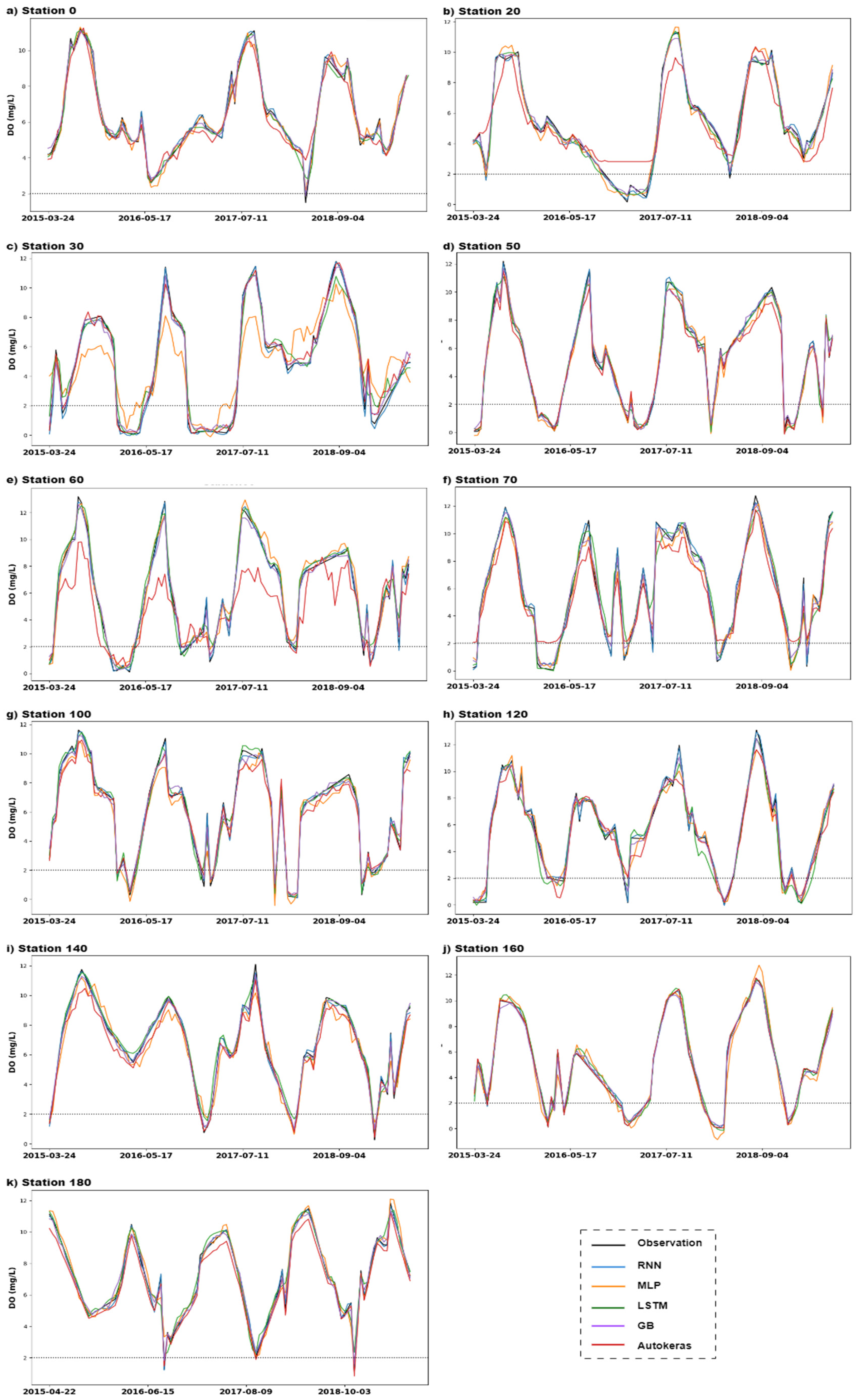
Figure 6 expands upon these results by providing a detailed comparison of the DO concentration predictions by the five models with in situ observations at various NRE stations. The plots demonstrate varying levels of accuracy and reliability, with some models performing better at certain stations. This spatial performance heterogeneity underscored the models’ sensitivities to site-specific dynamics. The RNN and GB model results were closest to the observations, illustrating their predictive capability. The MLP and LSTM models displayed competent predictions but with slightly higher deviations from the observed values.

Among the five models compared in Figure 6 and Table 2, the RNN’s predictions exhibited the closest alignment with the observations, particularly during hypoxia occurrence. The RNN model’s site-specific performance is further detailed in Figure 6, showcasing the model’s predictive accuracy across different stations. These subplots reinforced the model’s overall effectiveness, evidenced by its low MAE and high R² values.

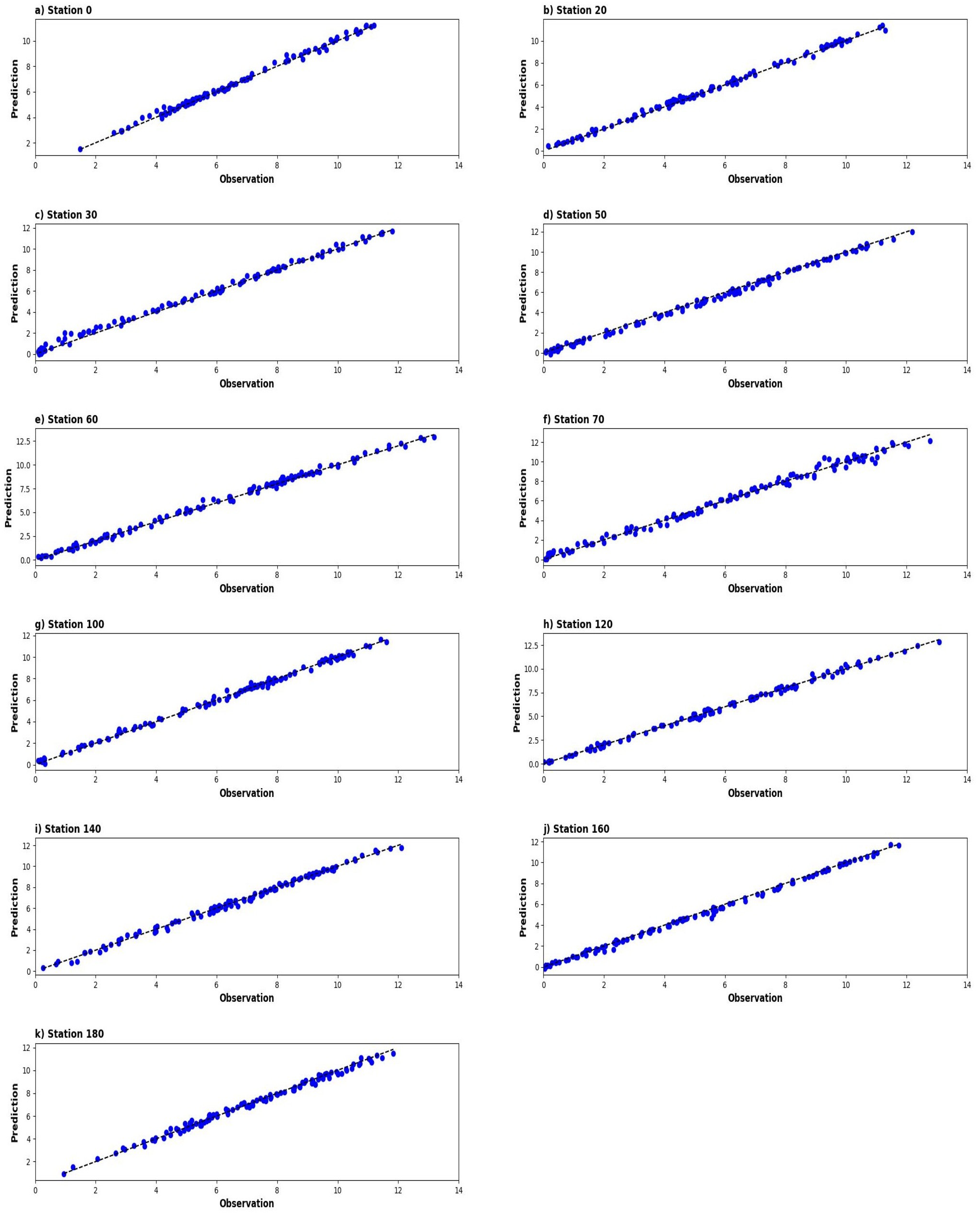
Lastly, Figure 7 delivers a direct comparison of the RNN-based DO predictions to actual values, visually represented through scatter plots for each station. The plots illustrated a high degree of correlation between the predicted and observed values, with most of the data points clustering near the diagonal line, indicative of high model accuracy.

4. Discussion

The RNN model’s outstanding performance, particularly its R² value of 0.99 at multiple stations, underscores its potential for capturing temporal dependencies and non-linear dynamics in environmental data. The sequential processing capability of RNNs allows for the integration of past information, which is crucial for time series prediction tasks such as DO concentration forecasting. This is visually corroborated in Figure 6, where the RNN predictions closely align with the observed values, and in Figure 7, where the scatter plots show a strong linear relationship between the predicted and observed DO concentrations.

The GB model also performed consistently well across different sites. Its ensemble approach, which combines multiple weak learners to form a strong predictive model, is particularly adept at handling complex, noisy datasets. As evidenced in Table 2, the GB model maintained high R² values, indicating its robustness in capturing the underlying patterns in the DO data. Conversely, the AutoKeras model exhibited the most considerable fluctuations in performance, with relatively high MAE and lower R² values. This variability could be attributed to the automated nature of the model selection process within AutoKeras, which may not always converge to the optimal model architecture for a given dataset, especially when the data contain intricate spatial and temporal correlations.

The MLP and LSTM models showed a competent but inconsistent performance. While these models are theoretically capable of modeling complex relationships, their performance may have been impacted by the hyperparameter settings, as suggested by the broader fluctuations in Figure 6 (for example, for station 30). However, there is potential that additional tuning or a more extensive search for the optimal architecture could improve their accuracy. Figure 6 presents a nuanced view of the model performance across various stations, highlighting how local station-specific environmental factors might influence the model accuracy. The differential performance across sites implies that while some models are generally accurate, their effectiveness can be station-specific. This suggests the necessity for localized model tuning to capture station-specific dynamics, which could be influenced by factors such as sensor placement or environmental disturbances.

The results also emphasize the importance of choosing appropriate performance metrics for model evaluation. While MAE provides a direct measure of the average prediction error, R² offers a normalized indication of the variance captured by the model. The high R² values for the RNN and GB models across most stations indicate not only their predictive accuracy but also their ability to generalize well across different environmental conditions.

It is noteworthy that the machine learning models are hindcast models, which use observed upcoming meteorological and discharge data. When the models are transferred to real-time operational forecasting, we can only use the forecasted upcoming meteorological and discharge data. Therefore, the operational forecast would have lower accuracy than the hindcast models presented in this study, determined by the accuracy of the predicted meteorological and discharge data.

5. Conclusions

This research implements five machine learning models to predict DO in the upcoming 2 weeks. The models exclude the influence of the accuracy of the predicted meteorological and discharge data on the DO forecast; however, they set the basis for the implementation of an operational forecast based on historical water sampling, predicted meteorology, and hydrology, which could provide local stakeholders—including water managers, field scientists, and fish anglers—with useful warning information about the occurrence of hypoxia. This research demonstrates the capability of artificial neural networks in modeling the dynamic and complex interactions affecting DO concentrations in the NRE, with the best performance by the RNN and GB. By focusing on selecting and testing various input variables, we reveal the significant accumulative and time delay impact of winds, especially wind in certain directions, and river discharge on DO. The exploration of different machine learning approaches suggests that there is no one-size-fits-all solution, and each model’s predictive capability may be enhanced or constrained by the dataset features and the complexity of the environment. Water quality forecasts can benefit from combining the strengths of different models and various types of feature engineering of the input features. In the future, we plan to (1) investigate the feature importance more, building a predictive model that requires fewer input features, potentially without the need for in situ water quality sampling but with comparable accuracy, and (2) optimize and simplify our models to better serve the research community for the local water resource management objectives by using predicted meteorological and hydrological data.

References

1. Paerl, H.W.; Rossignol, K.L.; Hall, S.N.; Peierls, B.L.; Wetz, M.S. Phytoplankton Community Indicators of Short- and Long-Term Ecological Change in the Anthropogenically and Climatically Impacted Neuse River Estuary, North Carolina, USA. Estuaries Coasts 2010, 33, 485–497. [Google Scholar] [CrossRef]
2. Latif, S.D.; Azmi, M.S.B.N.; Ahmed, A.N.; Fai, C.M.; El-Shafie, A. Application of Artificial Neural Network for Forecasting Nitrate Concentration as a Water Quality Parameter: A Case Study of Feitsui Reservoir, Taiwan. IJDNE 2020, 15, 647–652. [Google Scholar] [CrossRef]
3. Ziyad Sami, B.F.; Latif, S.D.; Ahmed, A.N.; Chow, M.F.; Murti, M.A.; Suhendi, A.; Ziyad Sami, B.H.; Wong, J.K.; Birima, A.H.; El-Shafie, A. Machine Learning Algorithm as a Sustainable Tool for Dissolved Oxygen Prediction: A Case Study of Feitsui Reservoir, Taiwan. Sci. Rep. 2022, 12, 3649. [Google Scholar] [CrossRef]
4. Zhi, W.; Feng, D.; Tsai, W.-P.; Sterle, G.; Harpold, A.; Shen, C.; Li, L. From Hydrometeorology to River Water Quality: Can a Deep Learning Model Predict Dissolved Oxygen at the Continental Scale? Environ. Sci. Technol. 2021, 55, 2357–2368. [Google Scholar] [CrossRef]
5. Vaquer-Sunyer, R.; Duarte, C.M. Thresholds of Hypoxia for Marine Biodiversity. Proc. Natl. Acad. Sci. USA 2008, 105, 15452–15457. [Google Scholar] [CrossRef]
6. Farrell, A.P.; Richards, J.G. Chapter 11 Defining Hypoxia: An Integrative Synthesis of the Responses of Fish to Hypoxia. In Fish Physiology; Richards, J.G., Farrell, A.P., Brauner, C.J., Eds.; Hypoxia; Academic Press: Cambridge, MA, USA, 2009; Volume 27, pp. 487–503. [Google Scholar]
7. Biddanda, B.A.; Weinke, A.D.; Kendall, S.T.; Gereaux, L.C.; Holcomb, T.M.; Snider, M.J.; Dila, D.K.; Long, S.A.; VandenBerg, C.; Knapp, K.; et al. Chronicles of Hypoxia: Time-Series Buoy Observations Reveal Annually Recurring Seasonal Basin-Wide Hypoxia in Muskegon Lake—A Great Lakes Estuary. J. Great Lakes Res. 2018, 44, 219–229. [Google Scholar] [CrossRef]
8. Rowe, M.D.; Anderson, E.J.; Wynne, T.T.; Stumpf, R.P.; Fanslow, D.L.; Kijanka, K.; Vanderploeg, H.A.; Strickler, J.R.; Davis, T.W. Vertical Distribution of Buoyant Microcystis Blooms in a Lagrangian Particle Tracking Model for Short-Term Forecasts in Lake Erie. J. Geophys. Res. Ocean. 2016, 175, 238. [Google Scholar] [CrossRef]
9. Moshogianis, A. A Statistical Model for the Prediction of Dissolved Oxygen Dynamics and the Potential for Hypoxia in the Mississippi Sound and Bight. Master’s Thesis, University of Southern Mississippi, Hattiesburg, MS, USA, 2015. [Google Scholar]
10. Katin, A.; Del Giudice, D.; Obenour, D.R. Temporally Resolved Coastal Hypoxia Forecasting and Uncertainty Assessment via Bayesian Mechanistic Modeling. Hydrol. Earth Syst. Sci. 2022, 26, 1131–1143. [Google Scholar] [CrossRef]
11. Chubarenko, I.; Tchepikova, I. Modelling of Man-Made Contribution to Salinity Increase into the Vistula Lagoon (Baltic Sea). Ecol. Model. 2001, 138, 87–100. [Google Scholar] [CrossRef]
12. Marcomini, A.; Sute, G.W., II; Critto, A. (Eds.) Decision Support Systems for Risk-Based Management of Contaminated Sites; Springer Science & Business Media: Berlin/Heidelberg, Germany, 2008; ISBN 978-0-387-09722-0. [Google Scholar]
13. Scavia, D.; Justić, D.; Obenour, D.R.; Craig, J.K.; Wang, L. Hypoxic Volume Is More Responsive than Hypoxic Area to Nutrient Load Reductions in the Northern Gulf of Mexico—And It Matters to Fish and Fisheries. Environ. Res. Lett. 2019, 14, 024012. [Google Scholar] [CrossRef]
14. Borsuk, M.E.; Higdon, D.; Stow, C.A.; Reckhow, K.H. A Bayesian Hierarchical Model to Predict Benthic Oxygen Demand from Organic Matter Loading in Estuaries and Coastal Zones. Ecol. Model. 2001, 143, 165–181. [Google Scholar] [CrossRef]
15. Katin, A.; Del Giudice, D.; Obenour, D.R. Modeling Biophysical Controls on Hypoxia in a Shallow Estuary Using a Bayesian Mechanistic Approach. Environ. Model. Softw. 2019, 120, 104491. [Google Scholar] [CrossRef]
16. Ahmed, A.A.M. Prediction of Dissolved Oxygen in Surma River by Biochemical Oxygen Demand and Chemical Oxygen Demand Using the Artificial Neural Networks (ANNs). J. King Saud. Univ.—Eng. Sci. 2017, 29, 151–158. [Google Scholar] [CrossRef]
17. Yu, X.; Shen, J.; Du, J. A Machine-Learning-Based Model for Water Quality in Coastal Waters, Taking Dissolved Oxygen and Hypoxia in Chesapeake Bay as an Example. Water Resour. Res. 2020, 56, e2020WR027227. [Google Scholar] [CrossRef]
18. Agatonovic-Kustrin, S.; Beresford, R. Basic Concepts of Artificial Neural Network (ANN) Modeling and Its Application in Pharmaceutical Research. J. Pharm. Biomed. Anal. 2000, 22, 717–727. [Google Scholar] [CrossRef]
19. Montgomery, D.C.; Peck, E.A.; Vining, G.G. Introduction to Linear Regression Analysis, 6th ed.; Wiley Series in Probability and Statistics; Wiley: Hoboken, NJ, USA, 2021; ISBN 978-1-119-57872-7. [Google Scholar]
20. Steinwart, I.; Christmann, A. Support Vector Machines; Springer: Berlin/Heidelberg, Germany, 2008. [Google Scholar]
21. Lu, H.; Ma, X. Hybrid Decision Tree-Based Machine Learning Models for Short-Term Water Quality Prediction. Chemosphere 2020, 249, 126169. [Google Scholar] [CrossRef]
22. Asadollah, S.B.H.S.; Sharafati, A.; Motta, D.; Yaseen, Z.M. River Water Quality Index Prediction and Uncertainty Analysis: A Comparative Study of Machine Learning Models. J. Environ. Chem. Eng. 2021, 9, 104599. [Google Scholar] [CrossRef]
23. Maier, H.R.; Jain, A.; Dandy, G.C.; Sudheer, K.P. Methods Used for the Development of Neural Networks for the Prediction of Water Resource Variables in River Systems: Current Status and Future Directions. Environ. Model. Softw. 2010, 25, 891–909. [Google Scholar] [CrossRef]
24. Antanasijević, D.; Pocajt, V.; Povrenović, D.; Perić-Grujić, A.; Ristić, M. Modelling of Dissolved Oxygen Content Using Artificial Neural Networks: Danube River, North Serbia, Case Study: Environmental Science & Pollution Research. Environ. Sci. Pollut. Res. 2013, 20, 9006–9013. [Google Scholar] [CrossRef]
25. Huang, J.; Liu, S.; Hassan, S.G.; Xu, L.; Huang, C. A Hybrid Model for Short-Term Dissolved Oxygen Content Prediction. Comput. Electron. Agric. 2021, 186, 106216. [Google Scholar] [CrossRef]
26. Nair, J.P. Analysing and Modelling Dissolved Oxygen Concentration Using Deep Learning Architectures. Int. J. Mech. Eng. 2022, 7, 12–22. [Google Scholar]
27. Bentéjac, C.; Csörgő, A.; Martínez-Muñoz, G. A Comparative Analysis of XGBoost. Artif. Intell. Rev. 2021, 54, 1937–1967. [Google Scholar] [CrossRef]
28. Sherstinsky, A. Fundamentals of Recurrent Neural Network (RNN) and Long Short-Term Memory (LSTM) Network. Phys. D Nonlinear Phenom. 2020, 404, 132306. [Google Scholar] [CrossRef]
29. Taud, H.; Mas, J.F. Multilayer Perceptron (MLP); Springer: Berlin/Heidelberg, Germany, 2017; Volume 2024. [Google Scholar]
30. Jin, H.; Song, Q.; Hu, X. Auto-Keras: An Efficient Neural Architecture Search System. In Proceedings of the 25th ACM SIGKDD International Conference on Knowledge Discovery & Data Mining, Anchorage, AK, USA, 4–8 August 2019; Association for Computing Machinery: New York, NY, USA, 2019; pp. 1946–1956. [Google Scholar]
31. Thompson, P.A.; Paerl, H.W.; Campbell, L.; Yin, K.; McDonald, K.S. Tropical Cyclones: What Are Their Impacts on Phytoplankton Ecology? J. Plankton Res. 2023, 45, 180–204. [Google Scholar] [CrossRef]
32. Stow, C.A.; Roessler, C.; Borsuk, M.E.; Bowen, J.D.; Reckhow, K.H. Comparison of Estuarine Water Quality Models for Total Maximum Daily Load Development in Neuse River Estuary. J. Water Resour. Plann. Manag. 2003, 129, 307–314. [Google Scholar] [CrossRef]
33. Paerl, H.; Pinckney, J.; Fear, J.; Peierls, B. Ecosystem Responses to Internal and Watershed Organic Matter Loading:Consequences for Hypoxia in the Eutrophying Neuse River Estuary, North Carolina, USA. Mar. Ecol. Prog. Ser. 1998, 166, 17–25. [Google Scholar] [CrossRef]
34. Wool, T.A.; Davie, S.R.; Rodriguez, H.N. Development of Three-Dimensional Hydrodynamic and Water Quality Models to Support Total Maximum Daily Load Decision Process for the Neuse River Estuary, North Carolina. J. Water Resour. Plann. Manage. 2003, 129, 295–306. [Google Scholar] [CrossRef]
35. Lin, J.; Liu, Q.; Song, Y.; Liu, J.; Yin, Y.; Hall, N.S. Temporal Prediction of Coastal Water Quality Based on Environmental Factors with Machine Learning. J. Mar. Sci. Eng. 2023, 11, 1608. [Google Scholar] [CrossRef]
36. Peirce, C.S. The numerical measure of the success of predictions. Science 1884, 4, 453–454. [Google Scholar] [CrossRef]
37. Raheli, B.; Aalami, M.; El-Shafie, A.; Ghorbani, M.; Deo, R. Uncertainty Assessment of the Multilayer Perceptron (MLP) Neural Network Model with Implementation of the Novel Hybrid MLP-FFA Method for Prediction of Biochemical Oxygen Demand and Dissolved Oxygen: A Case Study of Langat River. Environ. Earth Sci. 2017, 76, 503. [Google Scholar] [CrossRef]
38. Ismail, M.R.; Awang, M.K.; Rahman, M.N.A.; Makhtar, M. A Multi-Layer Perceptron Approach for Customer Churn Prediction. Int. J. Multimed. Ubiquitous Eng. 2015, 10, 213–222. [Google Scholar] [CrossRef]
39. Niroobakhsh, M. Prediction of Water Quality Parameter in Jajrood River Basin: Application of Multi Layer Perceptron (MLP) Perceptron and Radial Basis Function Networks of Artificial Neural Networks (ANNs). Afr. J. Agric. Res. 2012, 7, 4131–4139. [Google Scholar] [CrossRef]
40. Selvin, S.; Ravi, V.; Gopalakrishnan, E.A.; Menon, V.; Kp, S. Stock. In Price Prediction Using. LSTM, RNN and CNN-Sliding Window Model. In Proceedings of the 2017 International Conference on Advances in Computing, Communications and Informatics (ICACCI), Udupi, India, 13–16 September 2017; p. 1647. [Google Scholar]
41. Che, Z.; Purushotham, S.; Cho, K.; Sontag, D.; Liu, Y. Recurrent Neural Networks for Multivariate Time Series with Missing Values. Sci. Rep. 2018, 8, 6085. [Google Scholar] [CrossRef]
42. Hu, Z.; Zhang, Y.; Zhao, Y.; Xie, M.; Zhong, J.; Tu, Z.; Liu, J. A Water Quality Prediction Method Based on the Deep LSTM Network Considering Correlation in Smart Mariculture. Sensors 2019, 19, 1420. [Google Scholar] [CrossRef]
43. Friedman, J.H. Stochastic Gradient Boosting. Comput. Stat. Data Anal. 2002, 38, 367–378. [Google Scholar] [CrossRef]
44. Bolick, M.M.; Post, C.J.; Naser, M.-Z.; Mikhailova, E.A. Comparison of Machine Learning Algorithms to Predict Dissolved Oxygen in an Urban Stream. Env. Sci. Pollut. Res. 2023, 30, 78075–78096. [Google Scholar] [CrossRef]
45. Prasad, D.V.V.; Venkataramana, L.Y.; Kumar, P.S.; Prasannamedha, G.; Harshana, S.; Srividya, S.J.; Harrinei, K.; Indraganti, S. Analysis and Prediction of Water Quality Using Deep Learning and Auto Deep Learning Techniques. Sci. Total Environ. 2022, 821, 153311. [Google Scholar] [CrossRef]
Figure 1. Location and bathymetry of the NRE, with ModMon sampling sites represented by red dots.
Water 16 01998 g001
Figure 2. Comprehensive overview of the work plan. The NOAA NDBC station data include hourly meteorological data, including wind, air pressure, and air temperature data obtained from the NOAA NDBC station near Cape Lookout Bight, NC. In the diagram, “Today” represents model initialization time, and the models predict DO concentration in the upcoming 14 days (prediction time) based on ModMon sampling at a time before and closest to the model initialization time, the 14-day wind data, and 60-day river discharge before prediction time.
Water 16 01998 g002
Figure 3. Correlation of aggregated wind over time with DO concentration. N, NE, E, SE, S, SW, W, and NW represent winds in the sectors of N-NE, NE-E, E-SE, SE-S, S-SW, SW-W, W-NW, and NW-N, respectively. The horizontal axis represents the number of days prior to the prediction time over which the wind data are aggregated.
Water 16 01998 g003
Figure 4. Correlation of aggregated river discharge over time with DO concentration. The horizontal axis represents the aggregated river discharge over the number of days prior to the prediction time, with 0 representing the river discharge at the prediction time. YSI_DO is the observed DO at the prediction time.
Water 16 01998 g004
Figure 5. The architecture of the RNN model.
Water 16 01998 g005
Figure 6. Comparison of the DO (mg/L) predicted by five models with in situ observations at NRE stations (0, 20, 30, 50, 60, 70, 100, 120, 140, 160, and 180).
Water 16 01998 g006
Figure 7. Comparison of observations with the RNN-based DO predictions, the model with the best performance among the models implemented in the study. The dashed line represents the 1:1 line.
Water 16 01998 g007