Article

Prediction of Settling Velocity of Microplastics by Multiple Machine-Learning Methods

1
School of Marine Engineering Equipment, Zhejiang Ocean University, Zhoushan 316022, China
2
Ocean College, Zhejiang University, Zhoushan 316021, China
*
Author to whom correspondence should be addressed.
Water 2024, 16(13), 1850; https://doi.org/10.3390/w16131850
Submission received: 24 May 2024 / Revised: 26 June 2024 / Accepted: 26 June 2024 / Published: 28 June 2024

Abstract

:
The terminal settling velocity of microplastics plays a vital role in the physical behavior of microplastics, and is related to the migration and fate of these microplastics in the ocean. At present, the terminal settling velocity is mostly calculated by formulae, which also leads to a fewer studies on the use of machine-learning models to predict its settling velocity in this field. This study fills this gap by studying the prediction of the settling velocity by machine-learning models and compares it with the traditional formula calculation method. This study evaluates three machine-learning models, namely, random forest, linear regression, and the back propagation neural network. The results of this study show that the prediction results of the three machine-learning models are more accurate than those of traditional formula calculations, with an accuracy increase of 12.79% (random forest), 9.3% (linear regression), and 13.92% (back propagation neural network), respectively. At the same time, according to the results of this study, random forest is better than the other models in the mean absolute error and root mean square error evaluation indicators, which are only 0.0036 and 0.0047. This paper proposes three machine-learning methods to prove that the prediction effect of machine learning is much better than traditional formula calculations, thereby improving the shortcomings in this field. At the same time, it also provides reliable data support for studying the migration behavior of microplastics in water bodies.

1. Introduction

In recent years, microplastics have become an increasingly important topic of study for marine scientists. MPs are generally defined as plastic particles less than 5 mm in diameter and are widely distributed in rivers, lakes, oceans, and even the most remote places on Earth, such as the Arctic and Antarctic regions and the summit of Mt. Everest [1,2,3]. MPs can take the form of discs, fibers, films, particles, and fragments [4]. Because of their small size, they are easily mistaken for food by aquatic organisms. This can lead to their accumulation in the body and a variety of health problems [5]. Furthermore, toxic compounds and metals may attach to MPs’ surfaces and enter the food chain, exacerbating biological and, perhaps, human health concerns [6]. As a result, understanding the impact of plastic pollution on marine ecosystems and human health requires research into microplastics, and numerous studies have focused on their quantity, chemical composition, and biological impacts.
However, understanding the behavior of MPs in water is critical, with various studies using numerical modelling approaches to simulate and anticipate microplastic migration [7]. One of the most important features of microplastic (MP) migration in aquatic settings is settling velocity, since it is the major means of transport for negatively buoyant MPs in oceans. This parameter is critical for properly modeling MP migration in marine ecosystems [8,9]. Recent studies have shown that the terminal settling velocity of microplastics decreases with decreasing particle shape or particle size irregularity, when the particle size is in the range of 0.3 to 3.6 mm and the terminal settling velocity is less than 91 × 10−3 m/s. In this case, temperature and salinity do not affect the settling velocity [10,11].
Artificial intelligence is developing quickly, and its range of practical applications is growing, owing to the ongoing advancements in computer science and technology [12]. Numerous sectors, including but not limited to social media [13], medical sciences [14], electrical power [15], and climate [16], have demonstrated the value of artificial intelligence. Big data, deep learning, and machine learning are examples of artificial intelligence techniques that have been effectively used for predicting in a variety of sectors. Zhang advocated employing artificial intelligence to model the intricate interconnections between wind farms, molten salt energy storage, and s-COBC components. The trained AI model correctly predicted and projected the performance of the integrated renewable energy system, which improved grid integration and stability [17]. Han employed deep-learning approaches to swiftly predict the dispersion effects of diverse compounds, considerably increasing accuracy while significantly lowering numerical computations [18]. Xiao created a novel neural network model to quickly predict the compressive stress–strain curve of lattice metamaterials, and the findings outperformed existing approaches [19]. Artificial intelligence has shown outstanding success in predicting outcomes in a variety of domains.
The application of machine-learning (ML) models is pervasive in the domain of data analysis and prediction. This is particularly evident in the context of nonlinear classification and regression, where the ML approach offers significant advantages over traditional methods. The capacity to extract intrinsic information from large datasets can provide highly accurate prediction and analysis skills [20]. Machine-learning algorithms are well-suited to the task of detecting and utilizing a diverse range of data types. Machine-learning training may result in the creation of spatial models that are well-suited to a specific set of samples, As well as generating complex predictions or non-linear data distribution predictions. For instance, Rooki utilized a dataset comprising 88 samples to develop an artificial neural network with the objective of predicting the terminal settling velocity of solid spherical particles in Newtonian and non-Newtonian fluids [21]. Agwu developed an artificial neural network algorithm suitable for diamond chip particles of arbitrary shapes in the Reynolds number range of 1 to 100, providing a more convenient and faster alternative to the traditional method of predicting particle settling velocity using the drag-Reynolds number relationship coefficient [22]. Goldstein employed genetic programming learning to ascertain the particle settling velocity, which is a nonlinear function of the equivalent particle size, hydrodynamic viscosity, and particle immersion density. Additionally, the researchers tested the efficacy of training datasets of varying sizes to ascertain the minimum quantity of data required for training [23].
Currently, the use of machine learning in a variety of domains has demonstrated its dependability, but there has been little research on machine learning and marine microplastic migration. One of the most essential factors of microplastic migration is settling velocity, which is connected to microplastic density in the ocean. Thus, machine learning is required to predict the settling velocity of microplastics. In this study, three machine-learning models, RF, linear regression, and BPNN, were established, and the equivalent particle size, kinematic viscosity, liquid density, particle density, and shape factor were used as model input parameters, and the terminal settling velocity as the output value will be analyzed in comparison with the measured settling velocity in the laboratory. The dataset used in this study consists of two parts in total. The first part consists of the particles prepared by this study in the laboratory itself and their terminal settling velocities were measured. The other part is data collected from three papers, Yu et al. [6], Van Melkebeke et al. [24], and Francalanci et al. [25]. The two parts make up all the raw data used in this study. Moreover, we add the traditional formula to calculate the settling velocity. The results of machine learning are compared with the results of the traditional formulae to demonstrate the accuracy as well as the reliability of machine-learning prediction.

2. Materials and Methods

2.1. Particle Preparation

Microplastic particles with similar characteristic scales and physical properties to those found in the natural environment were selected for experiments. They were polystyrene (PS), purchased from Shanghai Boyu Plastics Co., Ltd. (Shanghai, China); polymethyl methacrylate (PMMA), purchased from Zhenjiang Chimei Chemical Co., Ltd. (Zhenjiang, China), Jiangsu, China; polyethylene terephthalate (PET) from China Resources Packaging Materials Co., Ltd. (Guangzhou, China); and acrylonitrile, butadiene, and styrene terpolymer (ABS) from Zhenjiang Chimei Chemical Co., Ltd. (Zhenjiang, China).
The polymer raw material particles were placed in an aluminum box in the laboratory and crushed with a file to obtain microplastic particles with a diameter of less than 5 mm. This method of microplastic preparation ensures that the particles retain their physical and chemical properties as much as possible, making them closely resemble microplastic particles found in the natural environment.
The size of each particle was measured using a vernier caliper with an accuracy of 0.01 mm. For each particle, three mutually perpendicular diameters were measured: the major axis (a), the middle axis (b), and the minor axis (c). These measurements were used to calculate the equivalent spherical diameter (ESD) [26], representing the size of the prepared microplastic particles.
E S D = a b c 3
Determination of particle density was performed using the pycnometer method. First, the mass of all particles (mp) was measured using an electronic balance. Next, a clean pycnometer was filled with pure water, and the bottle mouth was sealed slowly with a ground glass stopper fitted with a capillary tube. Any spilled water was wiped away with absorbent paper, and the mass of the pycnometer filled with water (mw) was recorded. The plastic particles were then carefully transferred into the pycnometer, and a thin metal rod was used to expel any small air bubbles present. The bottle was sealed with the stopper, excess water was wiped off with absorbent paper, and the mass of the pycnometer (mtotal) was measured again. The particle density was then calculated using the following formula:
ρ p = m p × ρ w m p + m w m t o t a l
The shape factor proposed by Corey is used to evaluate the deviation of laboratory-prepared particles from a perfect sphere and is one of the most commonly used parameters for this purpose. By definition, the shape factor of microplastic particles can be calculated using the following formula [27]:
c s f = c a b
In this study, the main physical properties of microplastic particles were selected as the parameters of the prediction model. These properties include equivalent particle size (ESD), form shape factor (csf), and density ( ρ ). The kinematic viscosity ( ν ), which affects particle settling, remains constant at 24 °C and was not included as an input parameter of the model in Table 1.
All 1183 microplastic particles prepared in the experiment were measured and calculated, resulting in 1183 sets of corresponding basic parameter data, as shown in Table 1. These parameters will serve as input variables for the machine-learning model.

2.2. Experimental Design

According to classical methods in sedimentology [28], the settling velocity of microplastic particles was measured in a cylindrical Plexiglas settling column. The settling column has a wall thickness of 1 cm, a height of 100 cm, and a circular cross-section with a diameter of 32 cm (choosing a settling column with a large cross-section helps minimize the impact of the container walls on particle settling velocity). The column is filled with pure water at a density of 1000 kg/m3. An automatic digital thermostat and heater are used to maintain the water temperature at a constant 24.5 °C (±0.5 °C) throughout the experiment. The ±0.5 °C tolerance is because the change in water viscosity caused by this slight temperature fluctuation is within 1.01%, rendering its impact on the terminal settling velocity negligible.
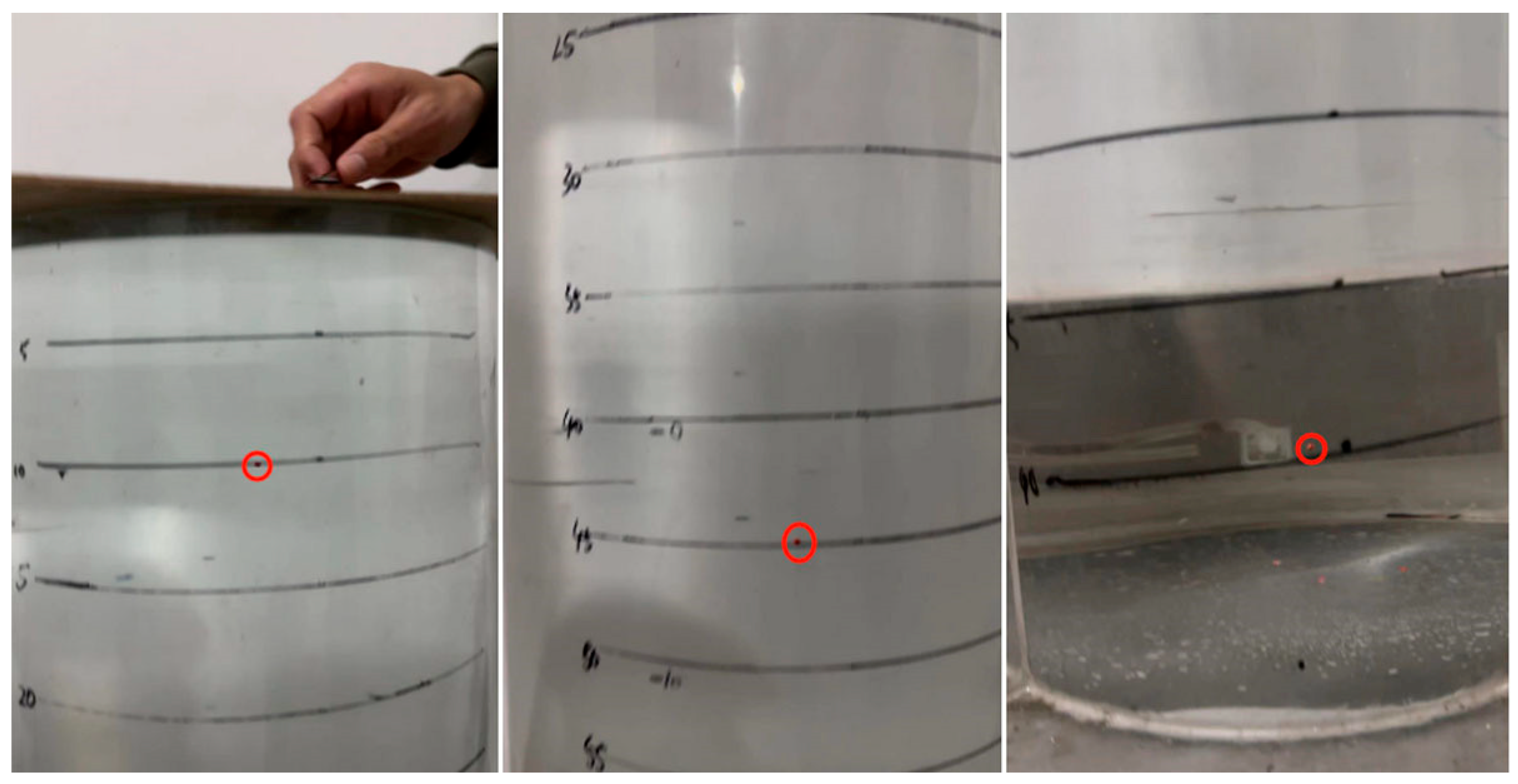
Before starting the experiment, the microplastic particles were soaked in the same liquid used in the settling cylinder at the same temperature to prevent any surface electrostatic discharge from hindering their settling. Using tongs, each particle was placed 1 cm below the water surface to eliminate the effects of surface tension, then released into the cylinder while the top was sealed with a lid to prevent convection. The depth at which the particles reach their terminal settling velocity is approximately 10 cm. Calibration marks were made 10 cm above and below the water surface in the settling column. The time required for the particles to traverse 80 cm vertically was recorded, and the settling velocity of each particle was subsequently calculated. The specific flow of the experiment is shown in Figure 1. The red circles in the figure indicate the settled particles.
The 1183 sets of microplastic terminal settling velocity data obtained through the above experimental steps will be compared with the settling velocity calculated by the equation and predicted by machine learning, as shown in Table 2:

2.3. Data Collection

This study obtained the fundamental parameters and measured the terminal settling velocity of all 1183 groups of microplastic particles through self-experimentation. The 1183 groups of data obtained from the self-experimentation will be used as the original dataset for the machine-learning model of this study. The corresponding settling velocity is presented in Table 3:
This study collected 927 sets of laboratory experimental data on the terminal settling velocity of microplastics from three papers: Yu et al. [6], Van Melkebeke et al. [24], and Francalanci et al. [25]. Nine types of plastic materials are included, including ESD (0.2 mm–5.44 mm). Plastics have eight different shapes (fragment, nodular, fiber, cylinders, sphere, pellet, film, and fish line), including CSF (0.01–0.99). The details are shown in Table 4:
The laboratory experimental data collected from the literature were combined with the data obtained from the experiments conducted in this study, forming the original dataset for this research.

2.4. Training and Testing Subsets

Machin- learning models typically require extensive training with large amounts of high-quality, representative data to accurately predict specific problems. Therefore, 70% of the data collected as described above was used to train the models. To evaluate the generalization performance of the model, the remaining 30% of the data was used to validate and test the trained model.

2.5. Formula Calculation

After research, a formula for predicting the settling velocity of microplastics was proposed [29]:
ω s = 1.0434 ( ρ p ρ f ρ f g ) 0.495 d n 0.777 C S F 0.710 ν 0.124
where ρ p is the density of microplastic particles, ρ f is the density of liquid, and υ is the Kinematic viscosity. The terminal settling velocity of microplastic particles can be calculated by this formula and compared with the measured amount.

3. Artificial Intelligence Model

3.1. Machine-Learning Model

3.1.1. Random Forest

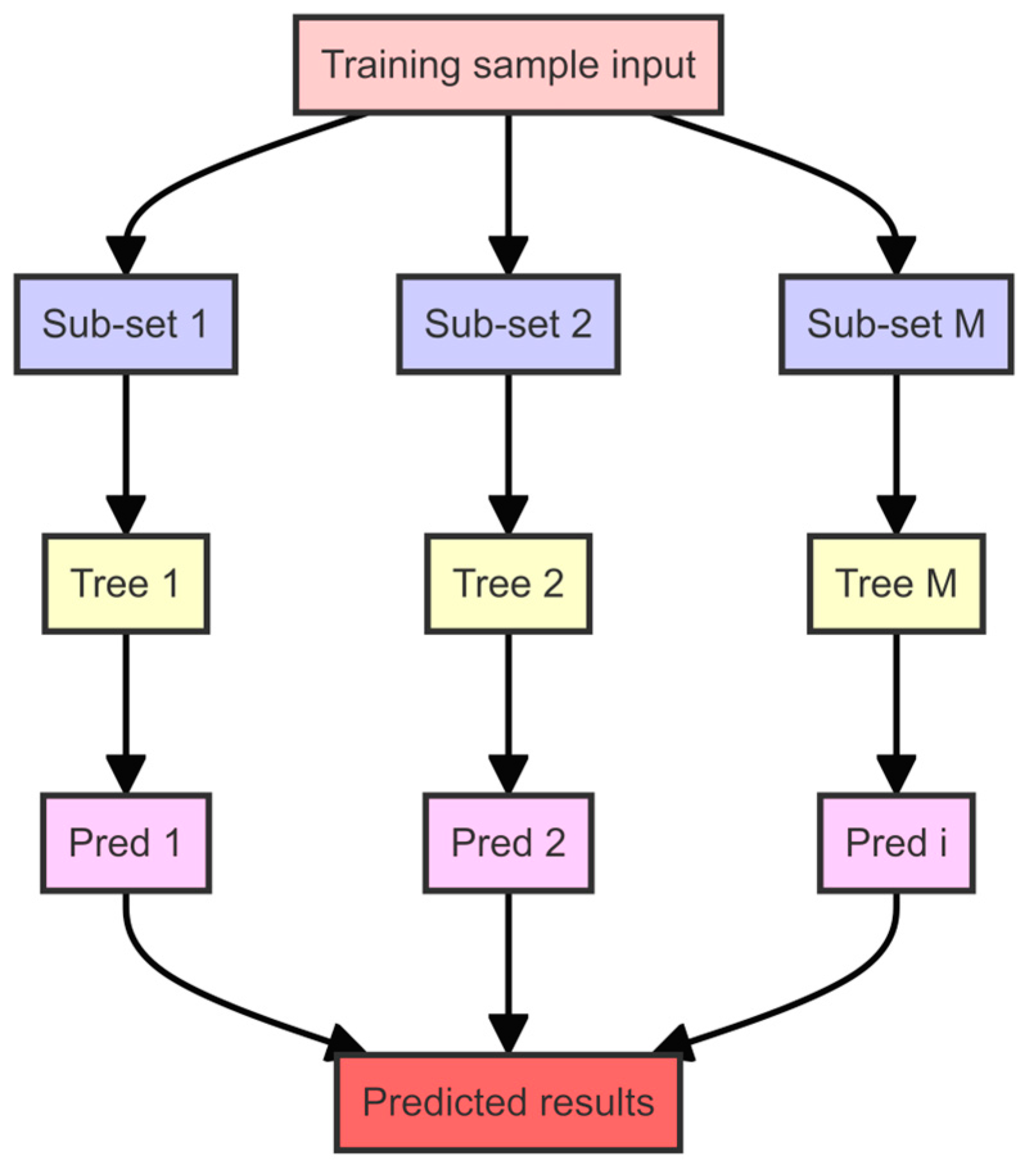
Random forest is a typical ensemble model based on the bagging method and consists of multiple weak learners. It works by randomly sampling and replacing samples from the original dataset to generate multiple sub-training sets, each corresponding to a weak learner. Each weak learner operates independently, identifying unique patterns and trends within its sub-training set to generate predictions.
To integrate the predictions of all learners, random forest employs various statistical methods. The final predictions are aggregated by averaging the outputs of each learner. This averaging process helps reduce biases or errors introduced by individual learners, thereby improving the overall model’s prediction accuracy. The schematic diagram of the random forest model is shown in Figure 2.

3.1.2. Linear Regression

Linear regression is a method of analysis that employs a regression equation (function) to model the relationship between one or more independent variables (features) and a dependent variable (target value). It entails preprocessing steps, such as data cleaning, handling missing values, and addressing outliers. The underlying principle is as follows:
h ( w ) = w 1 x 1 + w 2 x 2 + w 3 x 3 + b = w T x + b
In this context, “w” and “x” can be understood as matrices: w = ( b w 1 w 2 ) , x = ( 1 x 1 x 2 ) .

3.1.3. BPNN

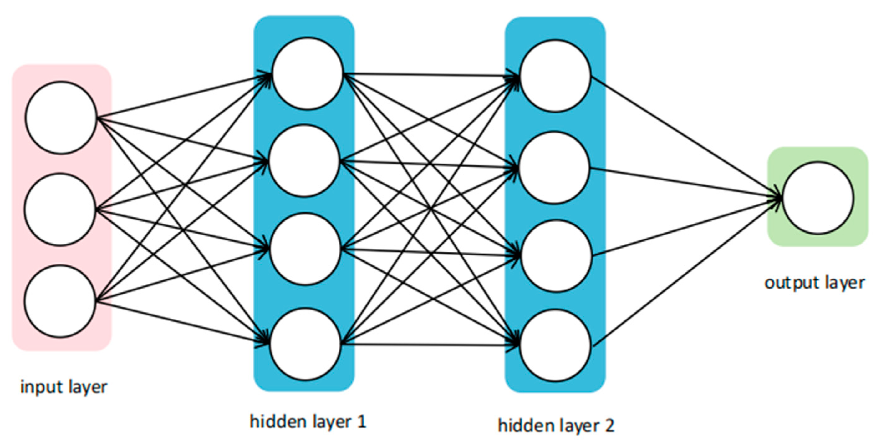
The back propagation neural network (BPNN) is an information transmission and computation system inspired by neuronal information processing. Its main structure includes input, hidden, and output layers. Through bi-directional propagation, BPNN constructs the intrinsic relationship between input data and experimental results.
During forward propagation (from the input layer to the output layer), the input data are transmitted from one neuron to the next through a specific linear equation. The equations are as follows:
y i = f v j = f i = 1 n w i j x i + b i
w i j represent the weights of neuron i for this layer and the next layer neuron j, respectively; and b i represents the deviation of the current layer. Equations (7) and (8) are used for the hidden and output layers.
f x = 1 1 + e x
f x = x
X indicates the data received.
During back propagation, the BPNN compares the predicted values with the actual values and uses a gradient descent algorithm to back propagate the resulting errors through the network. After hundreds of iterations, the model continuously adjusts the weights and biases, thus gradually improving the accuracy of the prediction. The schematic of the model is shown in Figure 3:

3.2. Model Development

3.2.1. Random Forest Algorithm

The raw data from Section 2.3 are employed as the dataset for machine learning. Seventy percent of the data from the training set was selected at random as the actual training dataset, and the feature matrices (trainX and testX) and the target vectors (trainY and testY) were extracted for the training and test sets, respectively. The training set comprises a number of features, including the equivalent particle size, kinetic viscosity, liquid density, particle density, and shape factor. In addition, the corresponding settling velocity is included as the target variable. The test set also contains analogous features with target variables. Subsequently, the model is subjected to hyperparameter tuning, whereby different combinations of hyperparameters are traversed. The hyperparameters include the number of leaf nodes of the decision tree (minleaf: 10–100) and the number of decision trees (ntrees = 3). The final “TreeBagger” model was trained on the entire training set using the optimal hyperparameters and subsequently tested on the test set. The predictive efficacy of the model on the test set was quantified, including the coefficient of determination of the predicted value versus the true value (R2), the mean absolute error (MAE), and the root mean square error (RMSE).

3.2.2. Linear Regression Algorithm

The original data from Section 2.3 are selected as the dataset for the model. The data were randomly divided into training and test sets in a ratio of 7:3. Since the linear regression model is highly vulnerable to the range of values associated with the features, feature scaling must be used to lessen the model’s sensitivity. The linear regression model was trained by fitting it using the “fillm” function. Subsequently, the trained model was employed to predict the test data, thereby generating predictions. Finally, the mean absolute error (MAE), root mean square error (RMSE), and correlation coefficient (R2) between the predicted and measured speeds were calculated.

3.2.3. BPNN

The raw data from Section 2.3 will be used as the dataset for the model. The data are preprocessed using normalization and divided into training and test sets in a 7:3 ratio, with random sampling used for selection. The input parameters include features such as the equivalent particle size, kinetic viscosity, liquid density, particle density, and shape factor, while the output settling velocity serves as the target variable. In order to address the hyperparameter aspect of the neural network model, a neural network comprising two hidden layers was constructed. The initial layer of the neural network, designated as the first hidden layer, contains 20 neurons. The subsequent layer, designated as the second hidden layer, contains 10 neurons. The maximum number of training rounds was set to 2000, and the training parameters, including the learning rate, were specified. Subsequently, the mean absolute error (MAE), root mean square error (RMSE), and coefficient of determination between the predicted output and the actual target variable are calculated at the conclusion of the model training.

3.3. Modeling for the Regular Models

In the context of machine learning, hyperparameters play a pivotal role in the model, as they directly influence the model’s performance. In order to optimize the performance of each model, it is necessary to determine the optimal hyperparameter settings through iterative experiments that are optimized based on the prediction error between the predicted and experimental values. Table 5 below provides a summary of the hyperparameter settings for the three models. Subsequently, the conventional models were trained using the aforementioned hyperparameters.

3.4. Evaluation of the Model

To evaluate the effectiveness and predictive power of machine-learning models, three metrics are used: mean absolute error, root mean square error, and correlation coefficient.

3.4.1. Mean Absolute Error (MAE)

M A E = 1 n i = 1 n y i y ^ i × 100 %
In this formula, n represents the sample size, y i denotes the measured velocity, and y ^ i denotes the predicted velocity. The absolute value in the calculation of the mean absolute error (MAE) avoids the issue of error cancellation and, thus, accurately reflects the magnitude of the prediction error. A lower MAE indicates a better predictive performance of the model.

3.4.2. Root Mean Square Error (RMSE)

R M S E = i = 1 n y i y ^ i 2 N
The root mean square error (RMSE) between the measured and predicted values is zero at the optimal fit, indicating a perfect fit between the prediction model and the measured data.

3.4.3. Coefficient of Determination (R2)

R 2 = 1 i = 1 n y ^ i y i 2 i = 1 n y ^ i y ¯ i 2
The parameter y ¯ i represents the average measured velocity. A value of R2 close to 1 indicates a high model accuracy and good predictive performance. Thus, a higher R2 value implies a better agreement between the predicted and observed sedimentation behavior.

4. Results and Discussion

4.1. Results

4.1.1. Formula Calculation Results Analysis

According to Equation (4), the settling velocities of all microplastic particles prepared in the laboratory were calculated using the equivalent particle size, kinematic viscosity, liquid density, particle density, and shape factor, where the density of the same liquid at the same temperature is constant, and the density of particles of the same material is constant. These calculated settling velocities were compared with the measured settling velocities obtained in the laboratory to analyze their consistency. The settling velocities of the four particles calculated by Equation (4) are shown in Table 6:
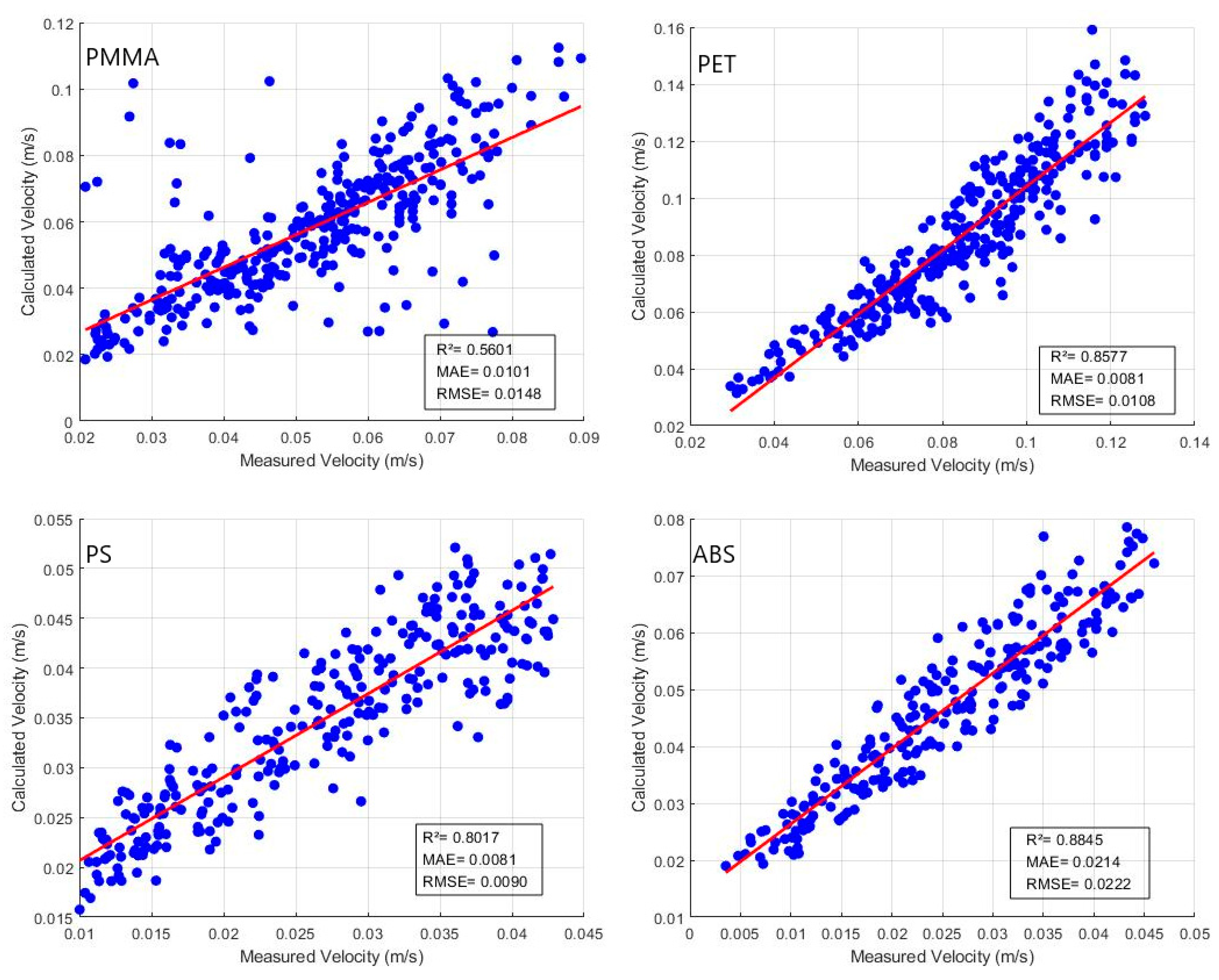
The settling velocity obtained by the equation was calculated in comparison with the measured settling velocity in the laboratory. The coefficient of determination (R2), mean absolute error (MAE), and root mean square error (RMSE) were calculated. The results are shown in Table 7 and Figure 4.
As shown in the table and figure above, the R2, MAE, and RMSE values calculated for the predicted and measured velocities were satisfactory. However, it was observed that the coefficient of determination for PMMA was only 0.5601, which was significantly lower than that for ABS particles, where R2 = 0.8845. For PS and PET particles, the R2 values were 0.8017 and 0.8577, respectively. Additionally, PS and PET particles exhibited lower MAE and RMSE values, with MAE: 0.0080 and 0.0081, and RMSE: 0.0089 and 0.0108, respectively.

4.1.2. Machine-Learning Prediction Results Analysis

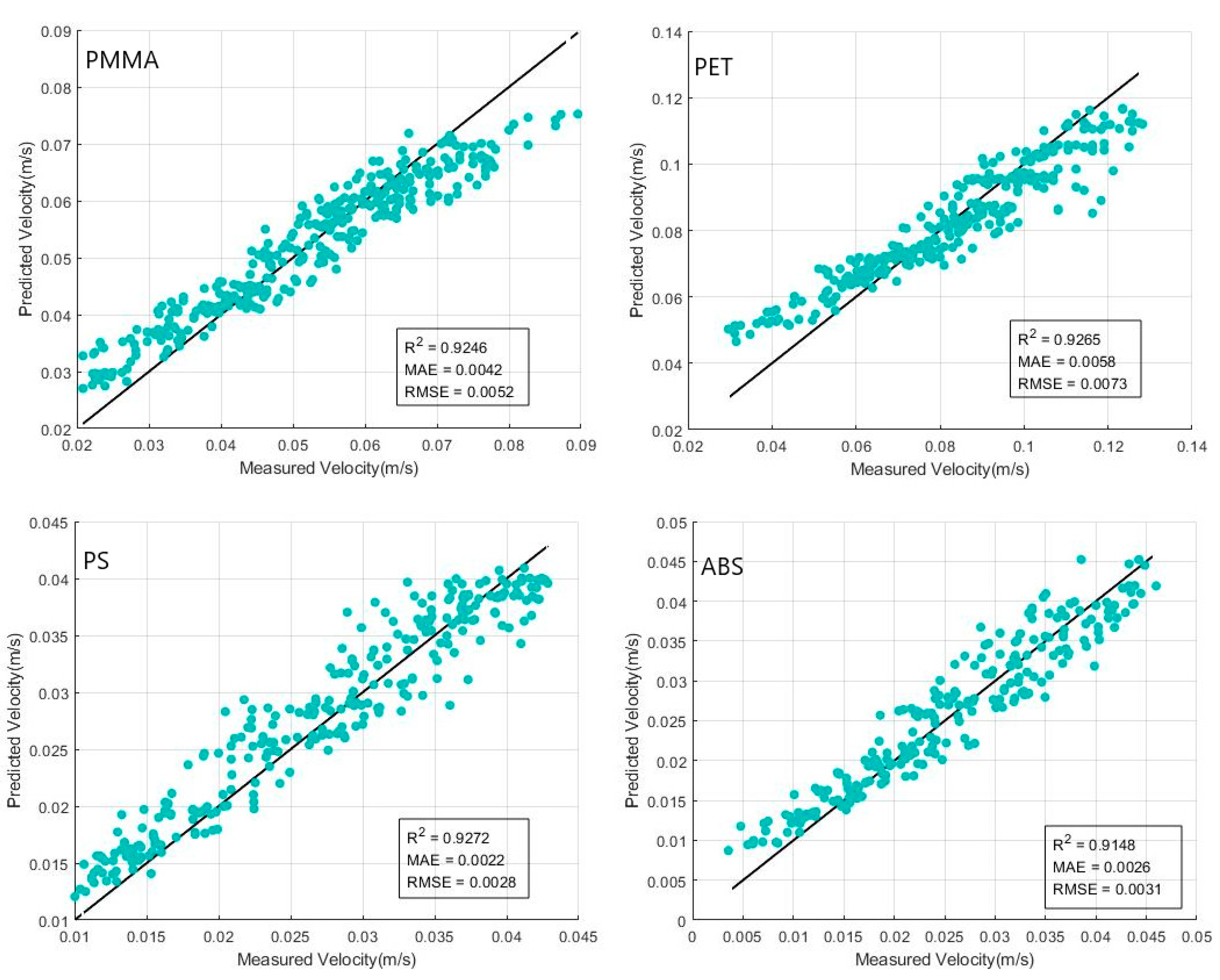
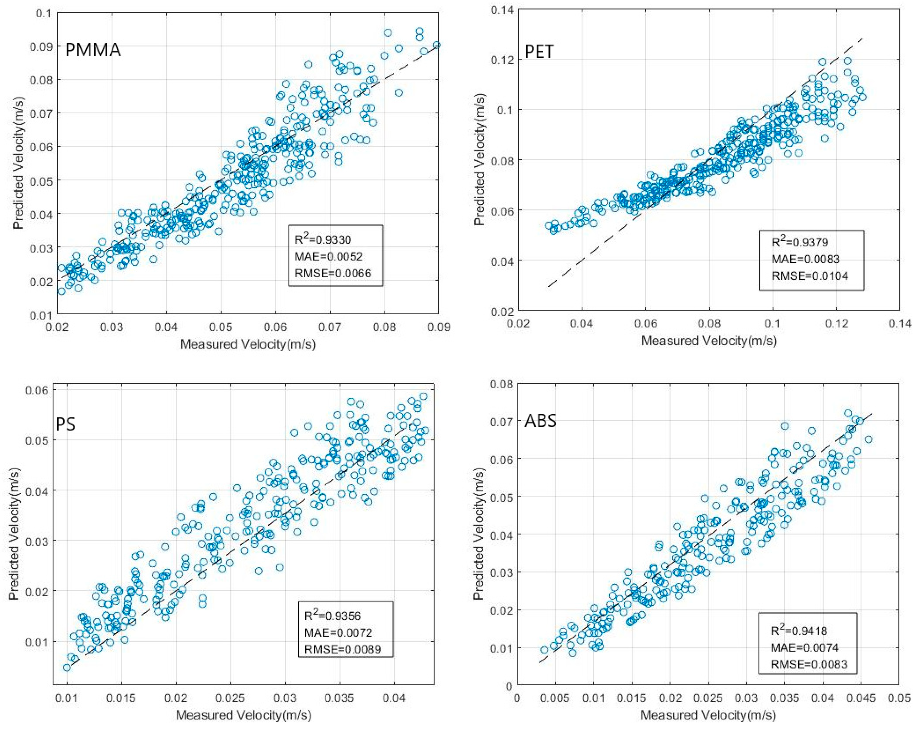
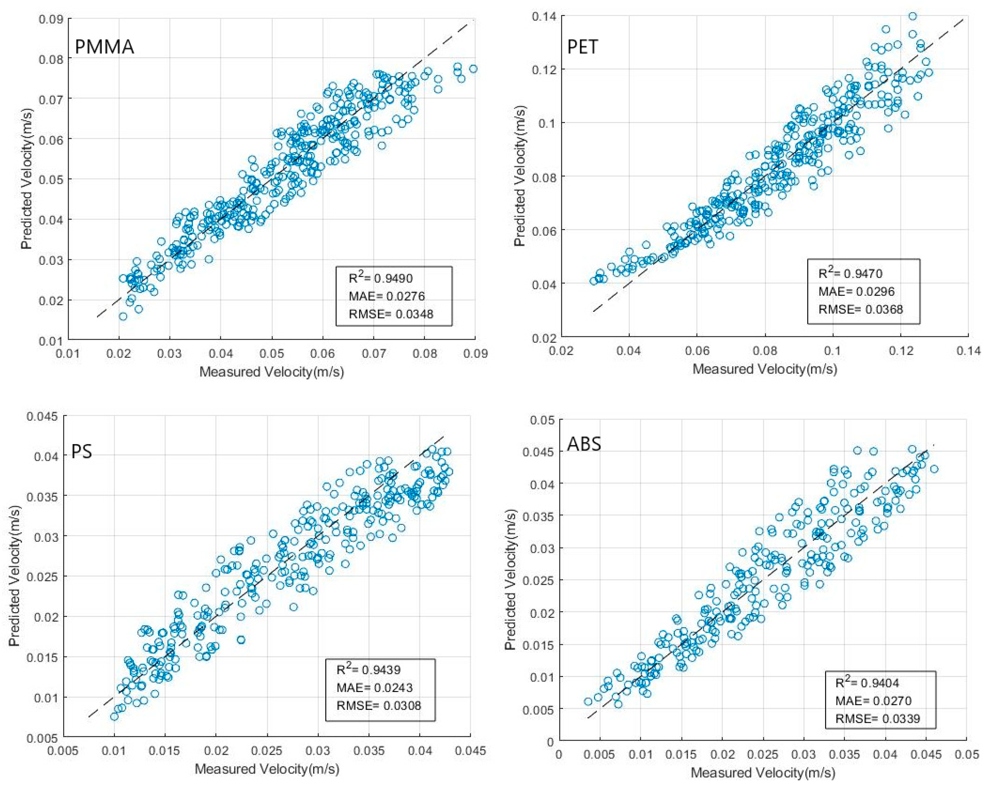
This study employs three machine-learning methods introduced earlier—random forest, a linear regression model, and a neural network model—to predict the terminal settling velocity of a dataset consisting of 1183 samples and 927 collected sample groups. The results from these models will be compared with those calculated using the formula. The results are shown in Figure 5, Figure 6 and Figure 7.
It can be clearly observed that the performance of machine learning is superior to that of the formula calculation, as indicated by the closer proximity of R2 values to 1, especially for PMMA particles. Additionally, the figure shows that the R2 values for the four types of microplastic particles obtained using the formula vary significantly, with a maximum difference of 0.2244. In contrast, the differences between the maximum and minimum R2 values obtained by the three machine-learning methods are 0.0124, 0.0086, and 0.0088, respectively. The maximum difference of only 0.0124 is substantially smaller than that produced by the formula, indicating that the settling velocity predicted by machine learning is more stable and exhibits less fluctuation. Moreover, the discrepancy between the settling velocity calculated by the formula and the measured velocity is even greater. It is also evident that machine-learning predictions follow a clear pattern: as the amount of the predicted particle data increases, the R2 value steadily improves. Conversely, the rules governing formula-based calculations and predictions are not as apparent.
In this study, prediction models for the terminal settling velocity of microplastics were established using three machine-learning algorithms. The correlation between the predicted and measured velocities was very high, with PMMA particles achieving R2 values of 0.93 (random forest), 0.93 (linear regression), and 0.95 (neural network). Moreover, the calculated MAE and RMSE were both very low, demonstrating the model’s effectiveness. The size of the training dataset significantly impacted the model’s predictive performance; larger datasets yielded more accurate predictions. Overall, the models proved robust and generalizable, accurately predicting the terminal settling velocity of microplastics. Additionally, the results indicate that the neural network algorithm may produce slightly lower MAE and RMSE values compared to the other two models. This sensitivity to outliers might be due to large deviations in the measured velocities of PMMA particles. It is also possible that the model’s complexity was insufficient to capture the intricate relationships within the data, leading to substantial differences between the predicted and measured velocities. Consequently, even with a high correlation coefficient, the MAE and RMSE values might still be large.

4.2. Discussion

By comparing the performance of the models in the Figure 8, the differences between the various models are readily apparent. Firstly, the closer the R2 is to 1, the more accurate the model’s predictions are and the better the model is. The results obtained from the formula are extremely inaccurate; the model is unstable, and has the lowest average R2. In contrast, the R2 of all three machine-learning models are much higher than the results calculated by the formula, and are very stable. The R2 value of BPNN is even closer to 0.95. Compared with RF and linear regression, the prediction is more accurate and stable. This further shows that, from the point of view of R2, the prediction result of machine learning is much better than the result of the formula calculation.
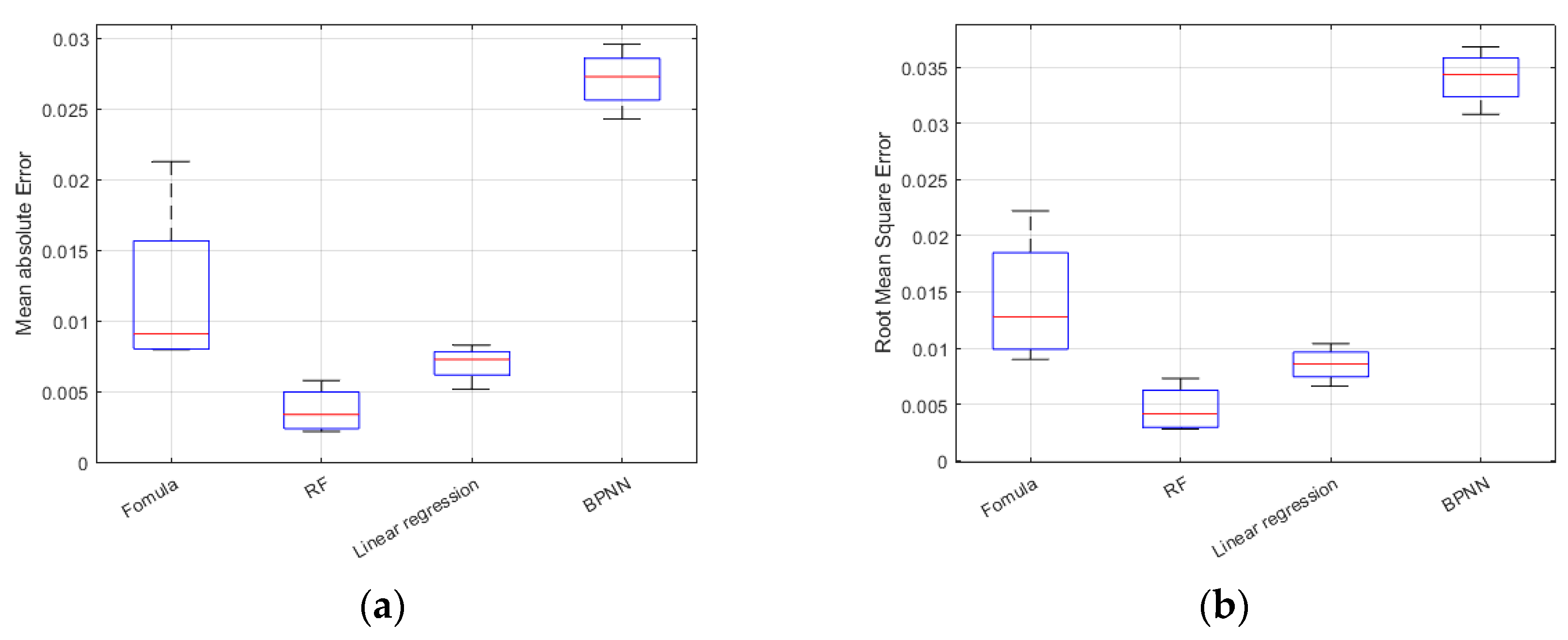
The accuracy of the model can be further analyzed in Figure 9a,b. RF has the lowest MAE and RMSE in predicting the settling velocity of the four microplastics, compared to both the formulae and the other two machine-learning models. The MAE accuracy of RF is 62% higher than that of the formulae (19%), the linear regression (37%), and the neural network (17%). RF also has the largest RMSE accuracy improvement of 61%. As can be seen from the graph, the results calculated by the formula have very large fluctuations, indicating poor stability. The neural network also has the highest MAE and RMSE values. It shows that these two models are less stable compared to RF and linear regression. In contrast, the differences for random forest and linear regression algorithms are much smaller: the MAE difference for random forest is 0.0036, the MAE difference for linear regression is 0.0031, the RMSE difference for random forest is 0.0045, and the RMSE difference for linear regression is 0.0038. This indicates that the predictions from these two algorithms are more stable and that their predictive performance is superior to that of the neural network model. At the same time, RF has the highest stability. As you can see from the graph, RF has the closest MAE and RMSE to 0. And the fluctuations are smaller compared to formulaic calculations and neural networks. Even though the fluctuation of linear regression is small, linear regression has relatively larger MAE and RMSE values. Overall, the random forest model is more accurate and stable.
The results section shows the prediction of the settling velocity for different species of experimentally prepared microplastics using the machine-learning model developed in this study. The laboratory-prepared particles all share the same shape but are made of different materials. Consequently, all the particles prepared in this study were considered as a whole for prediction, and the results were compared and analyzed against other existing machine-learning models and formula predictions.
From the comparisons in Table 8, it is evident that the machine-learning model developed in this study can accurately predict the settling velocity of regular microplastic particles. Moreover, the machine-learning prediction results in this study are superior to the traditional formulae for calculating settling velocity. The R2 value for the ANN model is significantly higher than the results reported by Rooki et al. [21]. Furthermore, the machine-learning prediction results in this study are also superior to those obtained using traditional formulae for calculating settling velocity. Additionally, the random forest model in this study outperforms the original formula in predicting the settling velocity. This demonstrates that the machine-learning model developed in this study provides superior predictions for the settling velocity of microplastic particles.

4.3. Parameter Importance Analysis

A sensitivity analysis of the input parameters was conducted separately for the three models, and the results are presented in Figure 10. The analysis revealed that the most significant factor affecting the settling velocity of microplastics is the density difference, followed by the equivalent particle size and the shape factor. This is attributed to temperature fluctuations during testing, which cause variations in the liquid density and, consequently, differences in the density of similar particles. Additionally, since different particles possess different densities, this further contributes to varying density differences. The equivalent particle size also plays a crucial role; as particle size changes, it directly influences the settling velocity.

5. Conclusions

A database consisting of 1183 sets of settling velocity data measured through experimental preparation in this study and an additional 927 sets collected from three literature sources was integrated to form a comprehensive dataset of 2110 sets. This dataset served as the foundation for developing and training the machine-learning models. The key conclusions drawn from this study are as follows:
The R2 values for the four types of microplastic particles calculated using the formula exhibit the largest variation, with a difference of 0.2244. In contrast, the maximum R2 difference obtained using machine-learning algorithms is only 0.0124. Additionally, the differences in MAE and RMSE using the formula are 0.0133 and 0.0132, respectively, which are significantly higher than those obtained with machine learning. Therefore, the comparison between the results of formula-based calculations and machine-learning predictions clearly indicates that the machine-learning algorithms can more accurately predict the settling velocity of microplastics.
The R2, MAE, and RMSE values obtained from all the machine-learning algorithms are relatively stable and follow the same trend. However, among the three machine-learning algorithms, the neural network algorithm is less effective than the RF algorithm and the linear regression algorithm, primarily due to the influence of outliers. Consequently, when comparing the three machine-learning algorithms, the neural network algorithm is slightly inferior to the other two. Furthermore, based on the MAE and RMSE comparisons, the RF algorithm is concluded to be the most stable machine-learning algorithm.
This study predicted the settling velocity of microplastic particles using three machine-learning models, which opens up new avenues for related research. However, future research can start by exploring more parameters that affect the settling velocity, or simulating water bodies with different temperatures to predict the settling velocity of particles, and different machine-learning models can also be developed to carry out the work of settling velocity prediction.

Author Contributions

Conceptualization, L.C. and Z.L.; methodology, Z.L.; software, Z.L.; formal analysis, L.C. and X.Z.; investigation, Y.G. and Y.H.; resources, D.W. and X.Z.; data curation, Z.L.; writing—original draft preparation, Z.L.; writing—review and editing, L.C., Y.G., Y.H. and Z.H.; visualization, Z.L.; supervision, Y.G., Y.H., D.W. and Z.H.; funding acquisition, L.C. All authors have read and agreed to the published version of the manuscript.

Funding

This work was supported by the National Natural Science Foundation of China (grant no. 51909237) and project of Zhoushan Science and Technology Bureau (grant no. 2020C11246).

Data Availability Statement

The datasets generated during and/or analyzed during the current study are available from the corresponding author on reasonable request.

Conflicts of Interest

The authors declare no conflicts of interest.

References

  1. Barnes, D.K.A.; Galgani, F.; Thompson, R.C.; Barlaz, M. Accumulation and fragmentation of plastic debris in global environments. Philos. Trans. R. Soc. Lond. B Biol. Sci. 2009, 364, 1985–1998. [Google Scholar] [CrossRef] [PubMed]
  2. Reed, S.; Clark, M.; Thompson, R.; Hughes, K.A. Microplastics in marine sediments near Rothera Research Station, Antarctica. Mar. Pollut. Bull. 2018, 133, 460–463. [Google Scholar] [CrossRef]
  3. La Daana, K.K.; Johansson, C.; Frias, J.P.G.L.; Gardfeldt, K.; Thompson, R.C.; O’Connor, I. Deep sea sediments of the Arctic Central Basin: A potential sink for microplastics. Deep. Sea Res. Part I Oceanogr. Res. Pap. 2019, 145, 137–142. [Google Scholar] [CrossRef]
  4. Khatmullina, L.; Isachenko, I. Settling velocity of microplastic particles of regular shapes. Mar. Pollut. Bull. 2017, 114, 871–880. [Google Scholar] [CrossRef] [PubMed]
  5. Avio, C.G.; Gorbi, S.; Milan, M.; Benedetti, M.; Fattorini, D.; D’Errico, G.; Pauletto, M.; Bargelloni, L.; Regoli, F. Pollutants bioavailability and toxicological risk from microplastics to marine mussels. Environ. Pollut. 2015, 198, 211–222. [Google Scholar] [CrossRef]
  6. Yu, Z.; Yang, G.; Zhang, W. A new model for the terminal settling velocity of microplastics. Mar. Pollut. Bull. 2022, 176, 113449. [Google Scholar] [CrossRef] [PubMed]
  7. Mason, R.A.; Kukulka, T.; Cohen, J.H. Effects of particle buoyancy, release location, and diel vertical migration on exposure of marine organisms to microplastics in Delaware Bay. Estuar. Coast. Shelf Sci. 2022, 275, 107990. [Google Scholar] [CrossRef]
  8. Critchell, K.; Lambrechts, J. Modelling accumulation of marine plastics in the coastal zone; what are the dominant physical processes? Estuar. Coast. Shelf Sci. 2016, 171, 111–122. [Google Scholar] [CrossRef]
  9. Ballent, A.; Purser, A.; de Jesus Mendes, P.; Pando, S.; Thomsen, L. Physical transport properties of marine microplastic pollution. Biogeosciences Discuss. 2012, 9, 18755–18798. [Google Scholar] [CrossRef]
  10. Kowalski, N.; Reichardt, A.M.; Waniek, J.J. Sinking rates of microplastics and potential implications of their alteration by physical, biological, and chemical factors. Mar. Pollut. Bull. 2016, 109, 310–319. [Google Scholar] [CrossRef]
  11. Chubarenko, I.; Bagaev, A.; Zobkov, M.; Esiukova, E. On some physical and dynamical properties of microplastic particles in marine environment. Mar. Pollut. Bull. 2016, 108, 105–112. [Google Scholar] [CrossRef] [PubMed]
  12. He, J.; Baxter, S.L.; Xu, J.; Xu, J.; Zhou, X.; Zhang, K. The practical implementation of artificial intelligence technologies in medicine. Nat. Med. 2019, 25, 30–36. [Google Scholar] [CrossRef] [PubMed]
  13. Abkenar, S.B.; Mahdipour, E.; Jameii, S.M.; Kashani, M.H. A hybrid classification method for Twitter spam detection based on differential evolution and random forest. Concurr. Comput. Pract. Exp. 2021, 33, e6381. [Google Scholar] [CrossRef]
  14. Liang, G.; Fan, W.; Luo, H.; Zhu, X. The emerging roles of artificial intelligence in cancer drug development and precision therapy. Biomed. Pharmacother. 2020, 128, 110255. [Google Scholar] [CrossRef] [PubMed]
  15. Liou, J.-L.; Liao, K.-C.; Wen, H.-T.; Wu, H.-Y. A study on nitrogen oxide emission prediction in Taichung thermal power plant using artificial intelligence (AI) model. Int. J. Hydrogen Energy 2024, 63, 1–9. [Google Scholar] [CrossRef]
  16. El-Mahdy, M.E.-S.; Mousa, F.A.; Morsy, F.I.; Kamel, A.F.; El-Tantawi, A. Flood classification and prediction in South Sudan using artificial intelligence models under a changing climate. Alex. Eng. J. 2024, 97, 127–141. [Google Scholar] [CrossRef]
  17. Zhang, C.; Yan, L.; Shi, J. Performance prediction of a supercritical CO2 Brayton cycle integrated with wind farm-based molten salt energy storage: Artificial intelligence (AI) approach. Case Stud. Therm. Eng. 2023, 51, 103533. [Google Scholar] [CrossRef]
  18. Han, X.; Zhu, J.; Li, H.; Xu, W.; Feng, J.; Hao, L.; Wei, H. Deep learning-based dispersion prediction model for hazardous chemical leaks using transfer learning. Process. Saf. Environ. Prot. 2024, 188, 363–373. [Google Scholar] [CrossRef]
  19. Xiao, L.; Shi, G.; Song, W. Machine learning predictions on the compressive stress–strain response of lattice-based metamaterials. Int. J. Solids Struct. 2024, 300, 112893. [Google Scholar] [CrossRef]
  20. Xu, Y.; Zhou, Y.; Sekula, P.; Ding, L. Machine learning in construction: From shallow to deep learning. Dev. Built Environ. 2021, 6, 100045. [Google Scholar] [CrossRef]
  21. Rooki, R.; Ardejani, F.D.; Moradzadeh, A.; Kelessidis, V.; Nourozi, M. Prediction of terminal velocity of solid spheres falling through Newtonian and non-Newtonian pseudoplastic power law fluid using artificial neural network. Int. J. Miner. Process. 2012, 110–111, 53–61. [Google Scholar] [CrossRef]
  22. Agwu, O.E.; Akpabio, J.U.; Dosunmu, A. Artificial neural network model for predicting drill cuttings settling velocity. Petroleum 2020, 6, 340–352. [Google Scholar] [CrossRef]
  23. Goldstein, E.B.; Coco, G. A machine learning approach for the prediction of settling velocity. Water Resour. Res. 2014, 50, 3595–3601. [Google Scholar] [CrossRef]
  24. Van Melkebeke, M.; Janssen, C.; De Meester, S. Characteristics and sinking behavior of typical microplastics including the potential effect of biofouling: Implications for remediation. Environ. Sci. Technol. 2020, 54, 8668–8680. [Google Scholar] [CrossRef] [PubMed]
  25. Francalanci, S.; Paris, E.; Solari, L. On the prediction of settling velocity for plastic particles of different shapes. Environ. Pollut. 2021, 290, 118068. [Google Scholar] [CrossRef] [PubMed]
  26. Kumar, R.G.; Strom, K.B.; Keyvani, A. Floc properties and settling velocity of San Jacinto estuary mud under variable shear and salinity conditions. Cont. Shelf Res. 2010, 30, 2067–2081. [Google Scholar] [CrossRef]
  27. Corey, A.T.; Albertson, M.L.; Fults, J.L.; Rollins, R.L.; Gardner, R.A.; Klinger, B.; Bock, R.O. Influence of Shape on the Fall Velocity of Sand Grains. Master’s Thesis, Colorado State University, Fort Collins, CO, USA, 1949. [Google Scholar]
  28. Hazzab, A.; Terfous, A.; Ghenaim, A. Measurement and modeling of the settling velocity of isometric particles. Powder Technol. 2008, 184, 105–113. [Google Scholar] [CrossRef]
  29. Wang, Z.; Dou, M.; Ren, P.; Sun, B.; Jia, R.; Zhou, Y. Settling velocity of irregularly shaped microplastics under steady and dynamic flow conditions. Environ. Sci. Pollut. Res. 2021, 28, 62116–62132. [Google Scholar] [CrossRef]
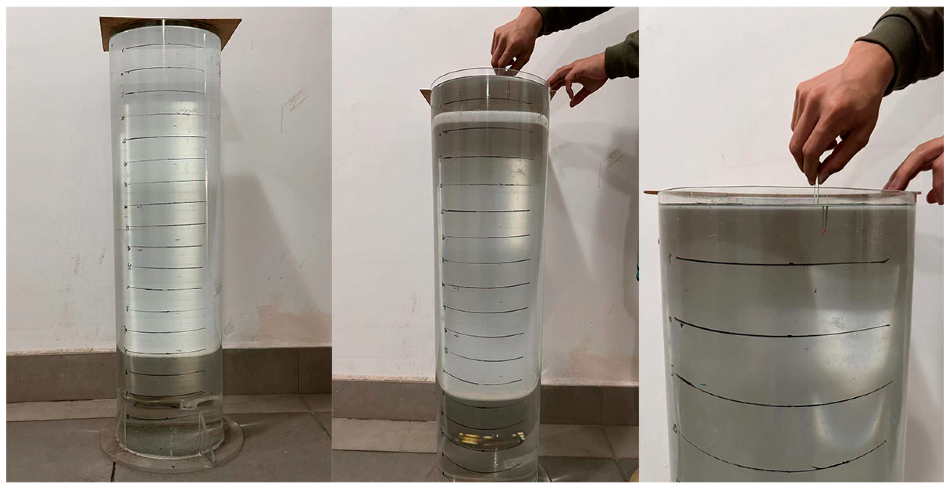
Figure 1. Settling velocity measurement diagram.
Water 16 01850 g001aWater 16 01850 g001b
Figure 2. Random forest schematic.
Water 16 01850 g002
Figure 3. Neural network schematic.
Water 16 01850 g003
Figure 4. Comparison chart between calculated velocity and measured velocity.
Water 16 01850 g004
Figure 5. Comparison chart of random forest prediction velocity and measured velocity.
Water 16 01850 g005
Figure 6. Comparison chart of linear regression predicted velocity and measured velocity.
Water 16 01850 g006
Figure 7. Comparison chart of neural network predicted velocity and measured velocity.
Water 16 01850 g007
Figure 8. Formula calculation and machine-learning R2 comparison diagram.
Water 16 01850 g008
Figure 9. (a) Formula calculation and machine-learning MAE comparison diagram. (b) Formula calculation and machine-learning RMSE comparison diagram.
Water 16 01850 g009
Figure 10. Parameter importance analysis.
Water 16 01850 g010
Table 1. Basic parameters of microplastic particles.
MpsQuantityESD (mm) ρ  (g/cm3)csf
Particle MaximumMinimumAverage Values MaximumMinimumAverage Values
PS2863.811.282.531.050.990.560.82
ABS2384.060.722.231.100.990.640.88
PMMA3404.660.812.331.190.980.390.74
PET3194.400.642.241.390.990.570.82
Table 2. Experimentally obtained terminal settling velocity.
MpsQuantityESD ω s (m/s)
Particle (mm)MaximumMinimumAverage Values
PS2861.28–3.810.04280.01000.0270
ABS2380.72–4.060.04590.00350.0254
PMMA3400.81–4.660.08950.02080.0520
PET3190.64–4.400.12820.02960.0838
Table 3. The particle parameters obtained in this experiment.
MpsQuantityESD ρ csf ω s
Particle (mm)(g/cm3) (m/s)
PS2861.28–3.811.050.56–0.980.0100–0.0428
ABS2380.72–4.061.100.64–0.990.0035–0.0459
PMMA3400.81–4.661.190.39–0.980.0208–0.0895
PET3190.64–4.401.390.57–0.990.0296–0.1282
Table 4. Characteristics of experimental MPS.
SourceParticle
Materials
ShapeData
Points
Equivalent Spherical Diameter [mm]Ρ (g/cm3)CSF ω (m/s)
Yu et al. [6]PETFragment950.56–2.791.390.06–0.340.019–0.07
PVCNodular, fiber1340.61–3.551.14–1.560.34–0.480.02–0.06
PCLCylinder, sphere371.03–2.021.1310.950.03–0.06
Fish line\2410.20–1.571.13–1.1680.16–0.990.003–0.05
PMMA\730.48–2.301.190.600.009–0.05
POM\680.55–2.251.420.110.01–0.04
PSFragment, pellet, cylinder510.50–2.121.05–1.0550.04–1.000.004–0.02
Van Melkebeke et al. [24]PETFragment201.37–2.801.370.07~0.830.01–0.10
PVCFiber200.64–1.611.430.02~0.160.007–0.02
PEFilm201.25–2.130.95–1.010.01~0.060.004–0.02
Francalanci et al. [25]PVCPellet381.68–4.941.084–1.250.25–0.850.069–0.156
PETPellet, fragment702.3–5.441.10–1.370.10~0.790.022–0.177
ABSPellet302.41–2.891.040.650.03–0.0467
PSPellet303.31–4.141.030.800.034–0.057
Table 5. Machine Learning Training Parameters.
ModelMain Parameter Setting
RFThe minimum number of leaf node samples: 1–30
Decision trees: 10–100
Maximum tree depth = 3
Linear regressionFunction: fillm
BPNNHidden layers: 2
Neurons in first layer: 20
Neurons in second layer: 10
Maximum epochs N = 2000
Learning rate = 0.1 0.1 0.001 N × n
Table 6. The particle settling velocity calculated by Equation.
MpsQuantity ω s (m/s)
Particle MaximumMinimumAverage Values
PMMA3400.1120.0190.058
PET3190.1590.0310.086
PS2860.0520.0160.035
ABS2380.0780.0190.047
Table 7. Correlation coefficient between calculated velocity and measured velocity.
MpsQuantityR2MAERMSE
Particle
PMMA3400.56010.01010.0147
PET3190.85770.00810.0108
PS2860.80170.00800.0089
ABS2380.88450.02130.0222
Table 8. Comparative analysis with other existing machine-learning models and formula predictions.
ReferencesModelR2MAERMSE
Rooki et al. [21]ANN0.947-0.038
Wang et al. [29]Formula0.86500.01080.0135
This studyRF0.97560.00360.0047
Linear regression0.94550.00780.0098
BPNN0.98540.03090.0383
Disclaimer/Publisher’s Note: The statements, opinions and data contained in all publications are solely those of the individual author(s) and contributor(s) and not of MDPI and/or the editor(s). MDPI and/or the editor(s) disclaim responsibility for any injury to people or property resulting from any ideas, methods, instructions or products referred to in the content.