Abstract
DEM-based approaches for assessing flood-prone areas have recently gained extensive attention due to their parsimony and cost-effectiveness. This work aims to test the capability of the Geomorphic Flood Index (GFI) to delineate flood-prone areas and the results performances while downscaling the calibration map. The accuracy was tested by examining the sensitivity to the exponent of the power function linking the flow depth in the river network and the upslope contributing area. Two approaches were selected: the first consisted of calibrating the GFI using a flood map generated through a 2D-SWE hydrodynamic model. The second consisted of correlating water depths with their corresponding upslope areas. The geomorphological model is able to effectively delineate flood susceptibility areas which, although on average larger than that obtained using the hydrodynamic model, provide a good starting point for any subsequent in-depth analysis. After calibration, an Objective Function of 0.21 and an Area Under the ROC Curve AUC = 92%, which is among the highest if compared with other cases in the literature, were obtained. Positive feedback was also obtained using a calibration map that covers only a rather limited portion of the basin. However, the small values of the scaling exponent obtained after calibration with the first method indicate substantial independence of the river depths from the upslope contributing areas. This leads to the belief that a simple power function is not particularly suitable for describing the relationships between these two variables.
1. Introduction
Extreme floods are one of the most destructive and widespread weather phenomena, causing serious losses every year in terms of human life, livelihoods, and economic damage worldwide [1]. In Europe, the concentration and expansion of anthropic communities and settlements on riverine plains tend to exacerbate the exposure and vulnerability to floods; in fact, a considerable percentage of the population is estimated to be dowel near a susceptible flood area [2,3]. As stated by some recent research [4], floods are anticipated to amplify in intensity and frequency in the future, due to climate change. However, since river floods are difficult to predict quantitatively, a susceptibility assessment can substantially help to mitigate the associated consequences [5,6,7,8].
The severe socioeconomic impacts of these phenomena have increased the need to better understand flood dynamics and seek potential methodologies for evaluating the consequences of these flood events worldwide. Recently, attention has been focused on flood mapping as a key tool that helps disaster risk reduction through a reduction in vulnerability and damages [9]. Flood maps are of great benefit in terms of flood-prone area definition, mitigation measure planning, and supporting decision-makers. Significant initiatives have been taken to efficiently intervene in the protection against these hazardous consequences. In Europe, for example, the European Flood Directive 2007/06/EC [10] is established to reduce the disastrous flood impact in coastal and catchment areas through flood mapping. Another similar endeavor in the United States is settled by the Federal Emergency Management Agency (FEMA) which has acknowledged the importance of these maps through creating flood insurance rate maps to provide flood-prone areas all over the entire United States [2,11,12,13].
Conventional methods for flood hazard assessment mainly include hydrological and hydrodynamic computational models. Their implementation makes the simulation of any scenario possible for various hydrological inputs, providing outcomes that are more or less reliable depending on the quality of available data [14,15,16]. Usually, lumped, semi-distributed, or distributed hydrologic models are utilized to generate flood hydrographs based on historical or probabilistic rainfall input. Hydrodynamic models, namely 1D, coupled 1D/2D, or fully 2D use the obtained runoff data as upstream boundary conditions to provide a spatial representation of flood dynamics in terms of water extent, depth, velocity, and arrival times. More recently, efforts have been made to couple hydrologic and hydraulic models for flood modeling purposes. Fattahi et al. [17] applied the 1D-2D GSSHA model to a 3450 km2 Iranian watershed, performing a sensitivity analysis on the accuracy of DEM, size of the grid, and density of streams. Ennouini et al. [18] used the rain-on-grid version of HEC-RAS 2D to assess hydraulic risk in small ungauged catchments. Nguyen et al. [19], Sanders et al. [20], and Aureli et al. [21] developed an original fully 2D coupled hydrologic–hydraulic model for flood hazard mapping.
To perform a reliable simulation, many input data are required: hydrological observation, land uses, geometrical description of the river network and the hydraulic structures included in the domain, and high-resolution DEMs. Some of these data may not be readily accessible due to the demand for considerable collection efforts and cost issues. Extensive input data implies a challenging calibration and validation procedure [22,23]. In addition, the obtained outcomes are usually associated with various sources of uncertainties. That either stems from the process of collecting and processing input data, and or the calibration of the model parameters. For these reasons, the application of fully 2D models is often limited to a small part of a river basin, on a spatial scale rarely larger than 100 km2 [24]. Recently, however, considerable advances have focused on High-Performance Flood Models to remove these limitations. Models that take advantage of the potentials of Graphics Processing Units (GPUs) are employed to significantly increase the speed of simulation compared to traditional CPUs, allowing the simulation of catchments of more than 1000 km2 [25,26] even up to the national scale [27]. Nonetheless, these efforts are still in their early stage of development [28,29].
The advancement of Digital Elevation Models (DEM) production in recent decades has increased the interest in simplified and parsimonious models. This appears due to the diversity and the accessibility to recent technologies for capturing and screening surface elevation terrain, like GPS, SAR, SAR interferometry, and especially LiDAR, which has facilitated the application of elevation-based geomorphological methods and made them more attractive [30]. These models do not claim to replace the previous ones but allow rapid evaluations to be carried out which can then be refined using physically based models, typically in specific locations.
Several researchers have exploited the geomorphic paleofloods footprint to develop simplified models for delineating flood plains. For instance, Dodov and Foufoula-Georgiou [31] introduced a geomorphological algorithm to determine the floodplain morphometric characteristics, and Nardi et al. [32] presented a high-resolution global dataset of Earth as a procedure for floodplain delineations. Before that, a scaling function for floodplain delineation was detailed in Nardi et al. [33,34] using a hydrogeomorphic method based on the relationship between the river depth and its relative accumulated contributive area. Nobre et al. [35] as well developed a hydro-geomorphological terrain approach known as Height Above the Nearest Drainage (HAND). Investigating the limitations and applications of geomorphic scaling functions, Annis et al. [36] analyzed the cause–effect relationship between the river water depth and drainage areas under various catchments geomorphology, different climate characteristics, and stream order ranking. Based on the topographic witness index created by Beven and Kirkby [37], Manfreda et al. [38] introduced a Modified Geomorphic Indicator (TIm) that relies on a threshold value to distinguish between areas susceptible to floods and dry areas within a basin. Afterward, in [39], the three of the above approaches including those of [30,33,38] were investigated comparatively to analyze the contribution of certain morphological determinant factors on flood susceptibility, such as elevation to the nearest channel, topographic convergence, and local slope. These techniques have been applied to two sub-basins of the Tiber River in central Italy. The results have exhibited that the geomorphological classifier TIm depicted the highest rate of true estimation followed by the classifier proposed by Degiorgis et al. [30]. The difference in elevation between a location of interest and the nearest stream centerline connected to it (H) shows the best performance as a single feature. The last results have been confirmed in the ulterior works [40,41] through an application in a West African basin. On the same line, Samela et al. [42] have also tested a group of geomorphological indicators that have been divided into single features and composed features. After finding that, among all the descriptors, the Geomorphic Flood Index (GFI) stands out with the best accuracy among the rest of the indicators for delineating flood-prone areas in ungauged environments, Samela et al. [43] developed a plugin called Geomorphic Flood Area (GFA) tool, which operates within the Geographic Information System Quantum (QGIS) environment.
The aim of this work particularly focuses on testing GFI for its ability to detect flood susceptibility, to examine its sensitivity to the hydraulic scaling function on which it is based, and to test this indicator’s accuracy in terms of flood-prone area identification while downscaling the calibration area. Care was devoted to verifying the basic assumptions and overcoming the limitations of the method. Indeed, many works based on geomorphological approaches take the validity of the scaling function for granted without calibrating its exponent. Furthermore, reference maps are often obtained with simplified 1D/2D models and rarely cover the entire watershed.
The workflow procedure used in this work takes advantage of the multitude of tools that GIS software provides. The input datasets required are a DEM and the reference flood hazard map that represents the maximum extent of flooded areas. Sometimes the method is applied with standard values of the scaling function. Sometimes, the methods or spatial resolution with which the reference map is obtained are not known or are not reliable enough to be used with confidence as a “gold standard” [42]. In this work, instead, a reference map was obtained using a high-resolution hydrodynamic model that, starting from precipitation, resolves the fully 2D shallow water equations both for overland and channelized flows [21].
The accuracy of flood-prone area prediction was tested by calibrating the scaling function exponent using two different methods: (i) minimizing the Objective Function (OF) through comparison between the GFI generated and reference binary hazard maps; and (ii) through a linear regression in the log-log space between water depths extracted from the reference map and the accumulate upstream areas. Moreover, to test the sensitivity of the method to downscaling the training area, three reference maps (Total, Center, and Downstream) were considered, and the results were compared to provide insights about the refinement of the flood-prone area delineation using the GFI approach.
This work is structured as follows: Section 2 presents the study area context and information. The dataset includes terrain elevation, hazard reference flood map, and the methodology workflow is detailed step by step in this section. The flood descriptor and its hydraulic scaling function, as well as the regression method, are also described in Section 2. The findings of the implemented methods are illustrated and discussed in Section 3, and the main conclusions are outlined in Section 4.
2. Materials and Methods
2.1. Study Area
The Enza River, the subject of this study, is a right-side tributary of the Po River, the main Italian river. Its total drainage basin covers an area of about 660 km2 with a length of the mainstream of 110 km; 65% of the total area of the basin is characterized by mountainous and hilly landscapes, while downstream areas are predominantly flat. Altitudes range between 1997 m a.s.l. on the southern mountainous ridge and 23 m a.s.l. at the confluence with the Po River. The annual average rainfall is about 1124 mm, unevenly distributed between the Apennine part to the south, where the average annual precipitation exceeds 2000 mm, and the flat area to the north, where the precipitation does not reach 800 mm per year. The case study of the present work focuses on the upstream mountainous area of the river basin (Figure 1) whose drainage area extends over 454 km2. The steep hillslopes of this part of the basin and the high precipitation amount give rise to short concentration times and consequently short and impulsive floods. These morphological characteristics align with the GFI capabilities, as it is known to perform effectively in pronounced topography, while in flatter areas its effectiveness decreases significantly [39,44]. Inside the basin considered, the rivers are not embanked and, apart from a few check dams in the smallest streams and some bank defenses along the main channel, they can still be considered quite natural. In December 2017 a particularly significant flood event occurred, the return period of which was estimated to exceed 200 years. In the downstream embanked river reach, downstream the area under investigation, floodwaters overtopped the right levee, and a breach occurred which caused the flooding of a vast urbanized territory, with considerable damage to structures and infrastructures [45].
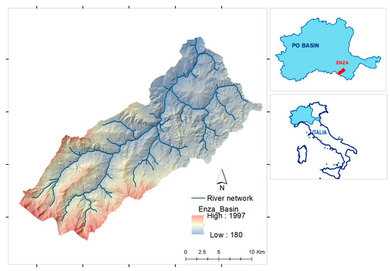
Figure 1.
Enza catchment and its location in Italy.
The hydrodynamic model used to derive the reference flooding map, and the tested geomorphological model, require a digital model of the entire basin to perform. For this aim, two topographic sources were used. The first is the AW3D30 model, with a spatial resolution of 1 arcsec (around 30 m), released by the Japanese space agency JAXA. The second is a DEM with a resolution of 1 m, resulting from a LiDAR survey carried out after the 2017 flood event. The first covers the entire basin, while the second covers only the main Enza river and valley (Table 1). The two DEMs were then merged and interpolated into a grid with a uniform spatial resolution of 5 m.

Table 1.
Sources and availability of used data.
For the application of the hydrodynamic model, it was not necessary to preliminarily fill the surface depressions of the DEM, as the model can perform the calculations even in their presence. In fact, the depressions fill naturally at the beginning of the simulated rainfall event. To speed up calculations, starting from the initial DEM, a structured BUQ multiresolution grid (Block Uniform Quadtree [25]) was built by maintaining the resolution of 5 m along the main watercourses and progressively decreasing it up to 40 m on the hillslopes, where high resolution is not of high importance (Figure 2).
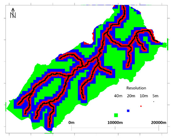
Figure 2.
Multiresolution Block Uniform Quadtree grid used for the 2d-SWE simulation.
Regarding the geomorphological model application, firstly, it was necessary to derive a “filled DEM”; this entails removing (real or artifacts) sinks, where all cells that contain an elevation value lower than their neighboring eight cells are “filled” to the elevation at which they will outlet water to an adjacent cell of lesser value [43]. This allows for the calculation of a “flow direction” matrix based on the slope gradient according to the D8 method [46] and, finally, for the generation of the “flow accumulation” grid file that corresponds to the number of the total upslope cells that flow into each downhill cell.
2.2. Hydrodynamic Model
To generate the flood reference map, the PARFLOOD-RAIN hydrodynamic model was used [21]. PARFLOOD [25] is a model built in the last ten years at the University of Parma that solves the set of complete 2D Shallow Water Equations (2D-SWE) [47], which in integral form can be written as follows:
where A is the area of the integration element; C is the element boundary; n is the outward unit vector normal to C; U is the vector of the conserved variables; H = (F, G) is the tensor of fluxes in the x and y directions; Sb, Sf, and Sr are the source terms representing, respectively, the bed slope, the frictional effect, and the rainfall rate. To avoid non-physical velocities at wet–dry fronts, the correction proposed by [48] is adopted:
in which η is the free surface elevation, h is the flow depth, and u and v are the velocity components in the x and y directions. The terms uh and vh identify the unit width discharges in the two coordinates directions, respectively; g is the gravitational acceleration; z is the bed elevation (η = z + h); r and f are the rainfall and infiltration rate, respectively.
The hyperbolic system of partial differential Equation (2) is discretized through an explicit finite volume scheme computing the numerical fluxes with the HLLC approximate Riemann solver [49]. The model achieves both first and second-order accuracy (in space and time), adopting for the latter case a depth-positive MUSCL extrapolation of the conserved variables values at the cell boundaries and a second-order Runge–Kutta time integration. The code is written in Compute Unified Device Architecture (CUDA) language, a framework introduced by NVIDIA to exploit both the GPU (the device) and the CPU (the host), ensuring speedups of two orders if compared with the CPU version. The model discretizes the computational domain with a Block Uniform Quadtree grid that allows adopting variable resolutions while preserving GPU efficiency. The PARFLOOD-RAIN version used in this work, introduced by [21], extends the simulation to the entire basin solving the 2D-SWE on the hillslopes, with a special treatment for considering small depths and high slopes.
The hydrodynamic model requires a proper boundary condition downstream, in correspondence with the modeled terminal section of the watercourse. In this case, a known stage-discharge relationship was adopted, placed in a section sufficiently downstream of the outlet so as not to influence the water levels in the area of interest. The model starts from specified initial conditions and receives contributions from precipitation, attributed in correspondence with the rain gauges, whose observations are subsequently spatialized with interpolation, or using precipitation radar maps anchored to the observations at the gauging stations (Table 1). The excess rainfall is derived through the application of the SCS Method, which allows the evaluation of the depth (mm) of the excess precipitation through the formulation based on CN values obtainable based on land use maps and hydrological soil groups available at the Emilia-Romagna Region public data repository (Table 1). Manning roughness values can be calibrated but limited to the main reach of the river, where some measuring stations are available. As for the secondary watercourses and hillslopes, however, the values of the roughness coefficient were attributed on the basis of the land use maps available at the mentioned public repository. The official soil polygon map downloaded by the repository was reworked by appropriately combining some similar subgroups. The Manning’s roughness coefficients for the numerical simulations were then deduced from the literature values based on the soil use (Table 1). The model can start from user-defined initial conditions or from the results of a previous simulation (hot-start). In the case considered here, the antecedent moisture conditions of the whole catchment were assumed as normal (AMC II), whereas, for the main riverbed, the initial conditions were derived from a preliminary simulation in steady flow corresponding to a modest value of discharge. Nonetheless, the influence of these initial conditions on the maximum water depths is negligible.
2.2.1. Event Simulation
As previously stated, this work considered the historical event that occurred in December 2017 (from 12:00 on 10 December 2017 to 6:00 on 12 December 2017). Space-distributed maps of rainfall depths with a 15 min time step were calculated using an inverse distance interpolation method starting from the data recorded from 16 rain gauges located within and in the close surroundings of the catchment. Figure 3 shows the map of the cumulative rainfall within the considered period. The maximum rainfall was recorded in the mountainous part of the basin. This occurrence is common, as rainfall is on average more abundant near the southern Apennines ridge, where the total annual rainfall is approximately three times higher than the flatter areas in the north.
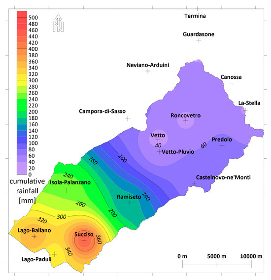
Figure 3.
Map of the cumulative rainfall from 12:00 on 10 December 2017 to 6:00 on 12 December 2017.
Effective rainfall was derived through the Soil Conservation Service Curve Number (SCS-CN) approach [50]. The CN (Class II) values (Figure 4a) were calculated by combining the data of soil types and land use available from the Emilia-Romagna region geoportal (Table 1). A land use map was also used to derive reasonable Manning coefficients (Figure 4b) for the entire catchment.

Figure 4.
(a) Values of curve number (normal antecedent moisture conditions AMC II) and (b) Manning roughness coefficients.
2.2.2. Flood Reference Map
The results of the hydrodynamic model consist of a sequence of maps containing the water depth and velocity field (vx and vy components of the velocity vector) for each element of the calculation grid at quite detailed output intervals (Δt = 15 min.) to correctly describe the dynamics of the flood under study. From these results, the map of maximum water depths can be obtained as the envelope of all the computed water depth maps and represents the maximum water depth reached in each cell during all the flood events (Figure 5). Figure 5 also shows the location of the water level gauging stations present in the area of interest, two of which did not return observations during the December 2017 event (Lonza and Selvanizza).
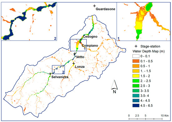
Figure 5.
Map of maximum water depths related to the event of 10–12 December 2017 in the whole Enza Basin with two zoomed areas.
For the 4 gauging stations that correctly measured water levels during the event, positioned along the main riverbed in correspondence with the areas covered by the high-resolution DEM, the results of the 2D hydrodynamic model are, as a whole, in satisfactory agreement with the observations. Unfortunately, no observations are available related to the flooded areas extent that could allow a comparison between the area actually flooded during the event and the flooding obtained using the hydrodynamic model. The validation performed on the basis of the available field data allowed us to assess the good behavior of the 2D hydrodynamic model in reproducing the flood event. Figure 5 shows the map of maximum water depths, which from here on will be used as a reference to calibrate the geomorphological model after being transformed into a binary map using a small water depth threshold (0.1 m).
The figure also shows two zooms extracted along the main river in the central and downstream parts of the basin. Some considerations can be outlined from the map. The maximum water depths (4.5 m and more, inset 2) are concentrated in the central part of the basin, where the valley is on average very narrow and presents some more accentuated rock narrowings and where, for more than one century, there has been debate about building the Vetto d’Enza dam. In the most downstream part, however, (inset 1) the valley widens and the maximum water depths significantly decrease.
2.3. Geomorphologic Model
GFI (Geomorphic Flood Index) is a descriptor for flood-prone area delineation that was introduced first in [39,41] and subsequently refined and used by many other authors [42]. A web application was also developed [2], as well as a GIS plugin [43]. This indicator generates a binary flood susceptibility map for a given catchment. It integrates terrain elevation information and utilizes hazard extent data as benchmark flood maps, readily available in small parts of the catchment, typically in the mainstream and rarely on the tributaries [43]. GFI, defined in Equation (3), is evaluated as the logarithm ratio between river depth (hr) and the elevation difference (H) between the site of interest and the nearest point of the stream network connected with it [51] (Figure 6).

Figure 6.
Description of the elements necessary to derive the Geomorphic Flood Index (GFI) (adapted from [2]).
To identify the connection of each point of the basin with the river network, it is necessary to define a complete map of the flow directions. This may represent a limitation of the method as in certain cases it is very difficult or even impossible to determine these directions, such as in the case of very flat basins or in the presence of embanked rivers.
Leopold and Maddock [52] showed that, at least in rivers not artificially constrained, the flow depth hr in the river network increases with the upslope contributing area Ar as a simple power function:
In Equation (4), hr is the water depth within the river at a certain location, Ar is the upslope contributing area, a is a scale factor, and n is a dimensionless scaling exponent. This behavior was subsequently explored and confirmed by other authors [33,53]. The exponent n of Equation (4) demonstrates variability across different catchments and normally ranges approximately between 0.24 and 0.45 [42,52,54]. In river networks with enough water level stations, the parameters a and n can be calibrated [42] by comparing historical Ar and hr values. In ungauged catchments, a suggested value of n (typically n = 0.354) in the literature is recommended, whereas the value of the parameter a does not affect the delineation of the flood-prone areas since ln(a) can be included in the computed GFI [51].
The first step in assessing the performance of the descriptor outcomes is the determination of the areas categorized as true positives (TP), false positives (FP), false negatives (FN), and true negatives (TN), referring to the benchmark flood map as illustrated in Figure 7. Subsequently, based on these values, the following rates were employed to create a difference between over or under-predictions and accurate predictions: rate of true positive: RTP = TP/(TP + FN); rate of true negatives: RTN = TN/(TN + FP); rate of false positives: RFP = FP/(TN + FP); rate of false negatives: RFN = FN/(TP + FN) and the Objective Function: OF = RFP + (1 − RTP). This latter expression value reflects the difference between the simulated flood-prone areas and the reference map. The closer the OF value is to 0, the more optimal the estimated flood-prone area becomes. Afterward, the ROC curve (Receiver Operating Characteristics [55]) relating RTP and RFP can be obtained [44] by changing the threshold value of GFI. The closer the curve is to the top left corner of the ROC space (RTP = 1, RFP = 0), the higher the accuracy of the classifier. The value of the Area Under the Roc Curve (AUC) varies between 0.5, relative to a random classifier, and 1, relative to a perfect classifier [39].
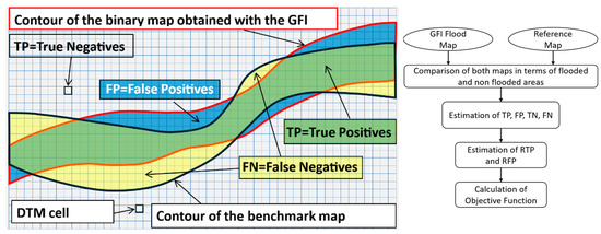
Figure 7.
Scheme for categorizing TP, FP, FN, and TN.
In the present study, two alternative approaches were used to estimate the “optimal” value of the exponent n of Equation (4). The first is based on an iterative process: once a value of the exponent n has been set (within its reasonable range of values), the threshold value of the GFI indicator is sought which minimizes the OF. The value of n is then varied until the absolute minimum of the OF is obtained.
The second approach [33] uses the non-binary reference map, i.e., the one containing the maximum water depth values obtained using the distributed hydrodynamic shallow water model, to select a consistent number of sections (cells) along the river network (main river and tributaries) to relate the maximum water depths (hr) with the upslope contributing areas (Ar). Through a linear regression on a log-log space, the values of the parameters a and n of Equation (4) are thus obtained, the second of which is then inserted into the geomorphological model procedure to generate the binary flood susceptibility map while always searching for the threshold value that minimizes the Objective Function.
In the literature, some authors (e.g., [41,56]) have mentioned that this GFI tool can provide good results using only a small portion of the basin area as a calibration map. To test the model’s ability and performance regarding this assumption, three calibration maps have been generated to different extents (Figure 8): the first one covers the entire basin area and serves as the main reference map; the second covers the central portion of the basin, still containing important information such as part of the mainstream, a confluence, and several tributaries; the third calibration map exclusively covers the downstream area of the basin since spatiotemporal information is commonly available only on the main river and the down floodplain portion of the catchment. The whole flowchart of the procedure is synthesized in Figure 9.
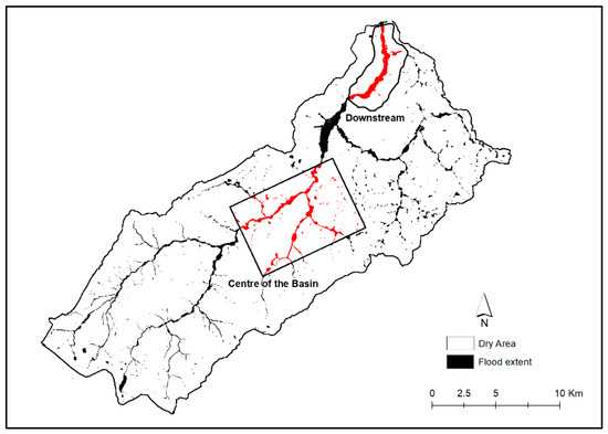
Figure 8.
Total binary map of the Enza basin used for GFI Calibration. The center and downstream calibration areas are also indicated.
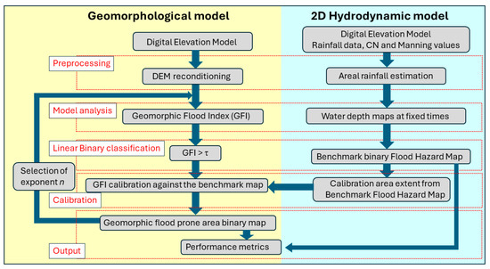
Figure 9.
Flowchart of the applied procedure.
3. Results and Discussion
Figure 10 shows the Objective Function as a function of the scale exponent n of Equation (4) obtained through the first approach previously described using the three different calibration area extents (Total, Center, Downstream). Some considerations can be made from the figure. First, it was not possible to identify a value of the scale exponent n that clearly minimizes OF. For this reason, a range of n values (n = 0.01–0.45) wider than that suggested in the literature (n = 0.24–0.45) was explored. The values of the scale exponent n between 0.01 and 0.05 essentially return the same value of OF (at least for the Total and Center calibration areas), while for higher values of n, OF increases. This result is quite unexpected, since such low values have never been reported in the literature (to the knowledge of the writers) and because this implies that hr is weakly dependent on the upslope contributing area Ar. As a possible explanation, it should be noted that the riverbed widens considerably as it proceeds downstream, where it assumes the aspect of a braided course free to wander which is entirely filled by the waters only during very rare occurrence floods. The results indicate that the highest accuracy of prediction is proven by the Total calibration map with a minimum Objective Function between 0.216 and 0.239, followed closely by the Center area that shows very similar performance (OF between 0.217 and 0.239), whereas the minimum performance is obtained by the Downstream calibration map, with the highest values of OF (between 0.22 and 0.26). It is worth explaining that the Center area contains more information in terms of prone areas diversity, such as tributaries, confluence, main river, and so on, which increases the accuracy of prediction. Despite these differences, even the Downstream calibration map proved sufficient accuracy according to the overall low values of OF. These results are in concordance with those obtained by [42], who suggest that the calibration of GFI can be exploited with a benchmark map covering a minimum of 2% of the total basin area.
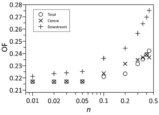
Figure 10.
Objective Function for different calibration area extent as a function of the scale exponent n.
Figure 11 displays the GFI’s performance as a flooding classifier indicator through the illustration of its Receiver Operating Characteristics curve related to the n = 0.01 value that refers to (almost) optimal performance obtained using the Total area. The best GFI threshold value (τ = −0.52) is indicated in red. The Area Under the ROC Curve (AUC) is equal to 0.92, which means a very good performance of the linear binary classifier.
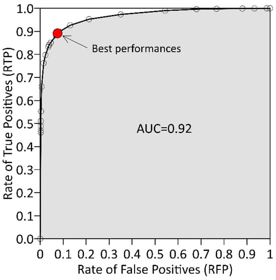
Figure 11.
Receiver Operating Characteristics curve obtained for the Enza Basin with n = 0.01.
These results can be compared with those obtained in [2] on the Po River sub-catchments, of which the Enza basin is part, with an average value of AUC = 0.84. On one hand, higher performance is obtained in the present study, on the other hand, the same value of AUC (0.92) was obtained over many sub-basins of the Ohio River in [12]. Furthermore, in the Paglia basin, Samela et al. [56] found a rate of positive prediction of RTP = 90% and a rate of False Positive RFP = 25%. The latter shows more likelihood of overprediction compared to our results.
Figure 12 shows the results obtained using the second approach to calibrate the value of the exponent n of Equation (4). From the map of maximum water depths obtained using the hydrodynamic model, the hr values were extracted for a few hundred sections (cells) with upslope contributing areas Ar > 2 km2. The high number of sections that can be extracted from the map obtained using the hydrodynamic model partly overcomes the lack of water stage gauging stations, the number of which is usually insufficient to calibrate the parameters of Equation (4). For this reason, some authors [37] have proceeded differently, starting from the estimate of a reasonable flow rate at the outlet and rescaling it along the stream network using the explicit equation of the Geomorphic Instantaneous Unit Hydrograph (GIUH) method and then estimating the water levels using the uniform flow discharge equation in the Manning form.
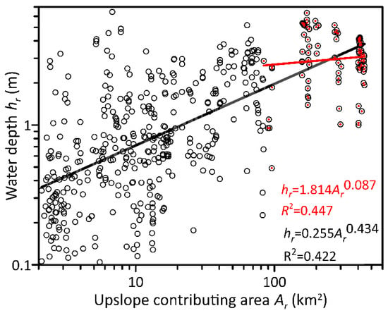
Figure 12.
Log-regression of water depth hr and contributing area Ar of the hydraulic scaling function to estimate exponent n.
The values obtained are reported in a log-log chart, where Equation (4) becomes a straight line, along with the best-fitting line. It is first worth noting the large dispersion of the points (R2 = 0.422), which is decidedly much larger than those obtained by [40] using historical USGS measurements in the Ohio Basin. Even for rather limited upslope contributing areas, of the order of 10 km2, very variable water depth values were found, which were probably caused by the presence of various narrowings and widenings due to the geological structure of the valley in which the Enza River flows. As has already been highlighted by observing the map of maximum water depths (Figure 5) obtained from the hydrodynamic model, this water depth variability partly contravenes Equation (4), which assumes that the flow depth in the river network increases with the upslope contributing area as a simple power function, which is the basis of many geomorphological models, including the one analyzed in this study. But the same behavior is found in many other basins of the Apennines’s tributaries of the Po River, where the presence of rock narrowings and/or paleoslides can even trigger the formation of ephemeral small lakes during major floods, which fill and empty within a period of a few hours [42].
From Figure 12, a tendency for hr to increase with Ar can be appreciated, and the slope of the regression line, i.e., the exponent n of Equation (4), takes on a value of 0.434, which is much more in line with the values found in the literature (0.406 for the Ohio basin analyzed by [40]). However, if the analysis is limited to the cells with significantly larger upslope contributing areas, downstream of some important confluences (Ar > 80 km2, red dots), the slope significantly decreases (n = 0.087, red line), coming very close to the “optimal” values obtained using the first approach. However, the large point dispersion persists (R2 = 0.447). By adopting n = 0.434 and searching for the optimal GFI threshold, a value of the Objective Function OF = 0.242 is obtained which, although not by much, is higher than the value OF = 0.217 obtained from the first calibration method of the exponent n of Equation (4).
One might argue that this poor correlation depends on the specific event considered here, whereas, if more events had been simulated, or if historical data had been available, the variability would have been more limited. In the basin under study, there are six level gauge stations, both on the mainstream and tributaries, most of which have been operating for at least twenty years. For each of them, the hydraulic authority has defined three hazard water level thresholds (low, medium, and high) roughly established based on the historical frequency of exceedance. Table 2 reports, for these stations, the contributing areas, the three aforementioned alert thresholds, the maximum water depth observed in the period of operation, and that recorded in the December 2017 event.

Table 2.
Level gauging stations, drainage areas, water level alarms, and maximum water levels recorded historically and in the December 2017 flood event.
Two stations failed to operate during the December 2017 event, while all others, except Station 3, recorded the maximum historical value. As can be seen from Table 2, the values of the alert thresholds and those of the recorded maximum depths have little or no correlation with the drained area: Fitting Equation (4) to these last data, the value n = 0.01 of scaling exponent would be obtained, but the very low value of the Coefficient of Determination (R2 = 0.027) confirms that, in this case, Equation (4) seems poorly suited to describe the relationship between hr and Ar.
Figure 13 shows the overlap of the benchmark map and the one obtained using the geomorphological model by adopting n = 0.01 (optimal value according to the first approach) and n = 0.454 (second approach). In both cases, the map obtained from the 2D hydrodynamic model of the entire basin was considered for calibration of the GFI threshold. The figure also shows three details that refer to upstream, intermediate, and downstream areas of the same basin.
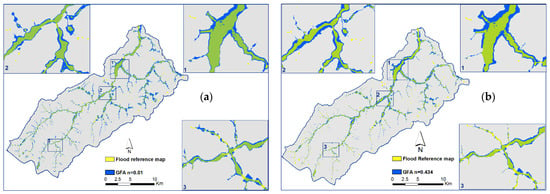
Figure 13.
Comparison between the reference flood map and the one obtained using the geomorphological model with the scaling exponent of Equation (4). (a) n = 0.01 and (b) n = 0.434. In both cases, the map obtained from the 2D hydrodynamic model of the entire basin was considered for calibration. Three zoomed areas are also shown.
In the first case (Figure 13a), the flooding map obtained using the geomorphological model is wider than the reference map almost everywhere, even if the extent of the overestimation is not very high. This overestimation may also be due to the fact that the benchmark map, obtained using the 2D SWE hydrodynamic model, is based on the original DEM, where the surface depressions (sinks) were not preliminarily filled as it was not necessary. Indeed, the numerical model is still able to perform the calculations in the presence of these surface depressions, which fill naturally in the first phase of the flood. For the application of the geomorphological model, it is instead necessary to “artificially” fill the surface depressions by locally altering the ground levels, thus producing a depressionless DEM, which is essential for identifying the drainage directions using the D8 method. Therefore, in these depressions false negatives are found (yellow dots in Figure 13a), which can partially compensate for the false positives along the main river network.
In the second case (Figure 13b), it can be appreciated that in the intermediate and downstream areas, the flooding map obtained using the geomorphologic model is larger than in the previous case. Conversely, the flood-prone area extent is narrower in the tributaries, where the contributing area is relatively small. This trend was expected, given the greater increase in hr with Ar in the second case, due to the higher n value. Furthermore, in the upstream zones, the hillslopes are steeper, so even large variations in estimated water levels result in smaller variations in the planimetric width of the estimated flooded map. In any case, the maps obtained using the geomorphological model are larger than the reference one obtained using the 2D hydrodynamic model. A possible explanation was given above.
As already mentioned, often a calibration map covering the entire basin is not available, and searching for the optimal scaling factor n is a somewhat laborious and time-consuming process. It was then explored whether, by adopting the standard value of n suggested in the literature (n = 0.354) and only a portion of the benchmark map for calibration, the binary map obtained using the geomorphological model was still acceptable. Figure 14 shows the comparison between the reference flooding map and the one obtained using the geomorphological model for the calibration of the Total (panel a), Center (panel b), and Downstream (panel c) maps. Table 3 summarizes the main values.
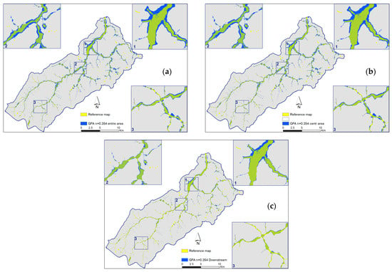
Figure 14.
Comparison between the reference flooding map and the one obtained using the geomorphological model with the scaling exponent of Equation (4) n = 0.354 adopting the (a) Total, (b) Center, and (c) Downstream maps for calibration. Three zoomed areas are also shown.

Table 3.
Threshold values of GFI, rate of true positive (RTP), and rate of false positive (RFP).
From Figure 14, it can be deduced that the results obtained using the Total and Center calibration maps are almost indistinguishable. The GFI threshold values differ only by the third decimal place and so do the values of RTP, RFP, and OF (Table 3). On the other hand, adopting the Downstream calibration map, the threshold value of GFI is higher (τ = −0.349), and the binary map is narrower everywhere. In all three cases, the performances (OF values) are worse than those obtained assuming the optimal value of the scale factor n. Apart from the numerical values, however, Figure 14c clearly shows that in the central and downstream parts, the binary map resulting from the geomorphological model fits better than the reference one. These results are expected, especially for the downstream area, as only this part was used for calibration. Depending on the area of greatest interest, it may be worth considering whether to use the entire calibration map, if available, or only a smaller part of it.
4. Conclusions
In this work, the performances of the geomorphological model based on the GFI to define flood-prone areas in the basin of the Enza River, a right tributary of the main Po River in Northern Italy, were evaluated.
To calibrate the model, a high-resolution reference map was obtained through a two-dimensional hydrodynamic model (PARFLOOD-RAIN), which solves the fully 2D-SWE both on the river network and on the hillslopes, starting from a distributed rainfall pattern. This constitutes, in the opinion of the writers, something new compared to what can be found in the literature, where very often the reference maps are quite approximate.
The accuracy of the method was tested by examining its sensitivity to the exponent of the hydraulic scaling function (Equation (4)) while reducing the calibration area.
The geomorphological model, once calibrated, is still able to provide a binary map of flood susceptibility which, although larger than that obtained using the hydrodynamic model on average, provides a good starting point for any subsequent in-depth analysis. In terms of binary classification efficiency, evaluated through the ROC curve analysis, the results depicted the high performance of the classifier with an AUC of 0.92.
These results align with the results obtained by Samela et al. [42] and are better than the average achieved by Tavares et al. [2] on the Po River sub-catchments with an AUC of 0.84.
Positive feedback was obtained by calibrating the geomorphological model with a reference map that covers only a rather limited portion of the basin. This feature is important, given that very often the available reference maps do not cover the entire basin, but only a part of it, typically the mainstream or a little more. If the calibration map contains enough information, the results are a little different from those that would be obtained using the full map.
In the studied case, the calibration of the exponent n of the scaling function by minimizing the Objective Function slightly improves the performance of the model, even if it leads to values of the scaling exponent n (0.01–0.05) that are decidedly lower than those suggested in the literature (0.24–0.45). These small values indicate a substantial independence of the river depth hr from the upslope contributing area Ar. The map of the maximum water depths obtained using the 2D hydrodynamic model, even if based on a single rainfall event, clearly shows how they are poorly correlated with the drained area, presumably due to the conformation of the valley, which presents various narrowings and widenings due to its geological structure. The same holds considering the historical values of six level gauge stations.
The search for the scaling exponent of Equation (4) through a linear regression in the log hr—log Ar space, instead, provides a value of the scaling exponent (n = 0.434) more in line with those suggested in the literature, but worsens, even if not by much, the OF between the map of flood susceptibility obtained using the geomorphological model and the reference map. Even in this case, however, a low correlation is observed between hr and Ar. This leads to the belief that Equation (4) is not particularly suitable for describing the relationships between these two variables, at least for the considered study area. The authors intend to verify whether this low correlation is a peculiar characteristic of the considered basin or, as they suspect, it could also be observed in other similar basins. To partially overcome this limitation, recently, some authors [13] have explored relationships between the river cross-sectional area (instead of hr) as a function of the contributing area Ar but did not find appreciable improvements. It cannot be ruled out that other approaches, which somehow consider the valley shape, such as the one proposed by [23], could provide better results. However, this risks nullifying the simplicity of the method, placing it in competition, at least for basins of comparable size to the one studied here, with complete 2D-SWE hydrodynamic models.
Author Contributions
Conceptualization, O.A. and P.M.; methodology, O.A. and P.M.; software, O.A., F.P. and F.A.; investigation, O.A. and P.M.; data curation O.A.; writing—original draft preparation, O.A. and P.M.; writing—review and editing, O.A., P.M., F.P. and F.A.; supervision, P.M.; funding acquisition, P.M. All authors have read and agreed to the published version of the manuscript.
Funding
Omayma Amellah and Paolo Mignosa acknowledge financial support from the PNRR MUR project ECS_00000033_ECOSISTER.
Data Availability Statement
The raw data supporting the conclusions of this article will be made available by the authors on request.
Conflicts of Interest
The authors declare no conflicts of interest.
References
- CRED/UNISDR. Human Cost of Weather Related Disasters 1995–2015; Centre for Research of the Epidemiology of Disasters: Université Catholique de Louvain, Ottignies-Louvain-la-Neuve, Belgium; The United Nations Office for Disaster Risk Reduction: Geneva, Switzerland, 2016; 30p, Available online: https://www.unisdr.org/2015/docs/climatechange/COP21_WeatherDisastersReport_2015_FINAL.pdf (accessed on 18 June 2024).
- Tavares da Costa, R.; Manfreda, S.; Luzzi, V.; Samela, C.; Mazzoli, P.; Castellarin, A.; Bagli, S. A Web Application for Hydrogeomorphic Flood Hazard Mapping. Environ. Model. Softw. 2019, 118, 172–186. [Google Scholar] [CrossRef]
- Wang, C.; Wang, K.; Liu, D.; Zhang, L.; Li, M.; Imran Khan, M.; Li, T.; Cui, S. Development and Application of a Comprehensive Assessment Method of Regional Flood Disaster Risk Based on a Refined Random Forest Model Using Beluga Whale Optimization. J. Hydrol. 2024, 633, 130963. [Google Scholar] [CrossRef]
- Alfieri, L.; Burek, P.; Feyen, L.; Forzieri, G. Global Warming Increases the Frequency of River Floods in Europe. Hydrol. Earth Syst. Sci. 2015, 19, 2247–2260. [Google Scholar] [CrossRef]
- Tehrany, M.S.; Pradhan, B.; Jebur, M.N. Flood Susceptibility Mapping Using a Novel Ensemble Weights-of-Evidence and Support Vector Machine Models in GIS. J. Hydrol. 2014, 512, 332–343. [Google Scholar] [CrossRef]
- Ebtehaj, I.; Bonakdari, H. A Comprehensive Comparison of the Fifth and Sixth Phases of the Coupled Model Intercomparison Project Based on the Canadian Earth System Models in Spatio-Temporal Variability of Long-Term Flood Susceptibility Using Remote Sensing and Flood Frequency Analy. J. Hydrol. 2023, 617, 128851. [Google Scholar] [CrossRef]
- Amiri, A.; Soltani, K.; Ebtehaj, I.; Bonakdari, H. A Novel Machine Learning Tool for Current and Future Flood Susceptibility Mapping by Integrating Remote Sensing and Geographic Information Systems. J. Hydrol. 2024, 632, 130936. [Google Scholar] [CrossRef]
- Amellah, O.; El Morabiti, K.; Maftei, C.; Papatheodorou, C.; Buta, C.; Bounab, A.; Ouchar Al-Djazouli, M. Topographic Indices and Two-Dimensional Hydrodynamic Modelling for Flood Hazard Mapping in a Data-Scarce Plain Area: A Case Study of Oued Laou Catchment (Northern of Morocco). Geocarto Int. 2022, 37, 13596–13617. [Google Scholar] [CrossRef]
- Ferrari, A.; Dazzi, S.; Vacondio, R.; Mignosa, P. Enhancing the Resilience to Flooding Induced by Levee Breaches in Lowland Areas: A Methodology Based on Numerical Modelling. Nat. Hazards Earth Syst. Sci. 2020, 20, 59–72. [Google Scholar] [CrossRef]
- European Union. Directive 2007/60/EC of the European Council and European Parliament of 23 October 2007 on the Assessment and Management of Flood Risks. Official Journal of the European Union 2007, 27–34. Available online: https://eur-lex.europa.eu/legal-content/EN/TXT/PDF/?uri=CELEX:32007L0060 (accessed on 18 June 2024).
- Hailemariam, F.M.; Brandimarte, L.; Dottori, F. Investigating the Influence of Minor Hydraulic Structures on Modeling Flood Events in Lowland Areas. Hydrol. Process. 2014, 28, 1742–1755. [Google Scholar] [CrossRef]
- Jafarzadegan, K.; Merwade, V. A DEM-Based Approach for Large-Scale Floodplain Mapping in Ungauged Watersheds. J. Hydrol. 2017, 550, 650–662. [Google Scholar] [CrossRef]
- Deiana, C.; Deidda, R.; Viola, F. Geomorphic Floodplain Mapping in Small Mediterranean Catchments Using LiDAR Data. Adv. Water Resour. 2023, 178, 104493. [Google Scholar] [CrossRef]
- Costabile, P.; Costanzo, C.; Macchione, F. Comparative Analysis of Overland Flow Models Using Finite Volume Schemes. J. Hydroinform. 2012, 14, 122–135. [Google Scholar] [CrossRef]
- Bellos, V.; Tsakiris, G. A Hybrid Method for Flood Simulation in Small Catchments Combining Hydrodynamic and Hydrological Techniques. J. Hydrol. 2016, 540, 331–339. [Google Scholar] [CrossRef]
- Magnini, A.; Lombardi, M.; Persiano, S.; Tirri, A.; Lo Conti, F.; Castellarin, A. Machine-Learning Blends of Geomorphic Descriptors: Value and Limitations for Flood Hazard Assessment across Large Floodplains. Nat. Hazards Earth Syst. Sci. 2022, 22, 1469–1486. [Google Scholar] [CrossRef]
- Fattahi, A.M.; Hosseini, K.; Farzin, S.; Mousavi, S.F. An Innovative Approach of GSSHA Model in Flood Analysis of Large Watersheds Based on Accuracy of DEM, Size of Grids, and Stream Density. Appl. Water Sci. 2023, 13, 33. [Google Scholar] [CrossRef]
- Ennouini, W.; Fenocchi, A.; Petaccia, G.; Persi, E.; Sibilla, S. A Complete Methodology to Assess Hydraulic Risk in Small Ungauged Catchments Based on HEC-RAS 2D Rain-On-Grid Simulations. Nat. Hazards 2024, 120, 7381–7409. [Google Scholar] [CrossRef]
- Nguyen, P.; Thorstensen, A.; Sorooshian, S.; Hsu, K.; AghaKouchak, A.; Sanders, B.; Koren, V.; Cui, Z.; Smith, M. A High Resolution Coupled Hydrologic–Hydraulic Model (HiResFlood-UCI) for Flash Flood Modeling. J. Hydrol. 2016, 541, 401–420. [Google Scholar] [CrossRef]
- Sanders, B.F.; Schubert, J.E. PRIMo: Parallel Raster Inundation Model. Adv. Water Resour. 2019, 126, 79–95. [Google Scholar] [CrossRef]
- Aureli, F.; Prost, F.; Vacondio, R.; Dazzi, S.; Ferrari, A. A GPU-Accelerated Shallow-Water Scheme for Surface Runoff Simulations. Water 2020, 12, 637. [Google Scholar] [CrossRef]
- Horritt, M.S.; Bates, P.D. Evaluation of 1D and 2D Numerical Models for Predicting River Flood Inundation. J. Hydrol. 2002, 268, 87–99. [Google Scholar] [CrossRef]
- Manfreda, S.; Samela, C.; Sole, A.; Fiorentino, M. Flood-Prone Areas Assessment Using Linear Binary Classifiers Based on Morphological Indices. In Vulnerability, Uncertainty, and Risk; American Society of Civil Engineers: Reston, VA, USA, 2014; pp. 2002–2011. [Google Scholar]
- Wingfield, T.; Macdonald, N.; Peters, K.; Spees, J.; Potter, K. Natural Flood Management: Beyond the Evidence Debate. Area 2019, 51, 743–751. [Google Scholar] [CrossRef]
- Vacondio, R.; Dal Palù, A.; Ferrari, A.; Mignosa, P.; Aureli, F.; Dazzi, S. A Non-Uniform Efficient Grid Type for GPU-Parallel Shallow Water Equations Models. Environ. Model. Softw. 2017, 88, 119–137. [Google Scholar] [CrossRef]
- Xia, X.; Liang, Q.; Ming, X. A Full-Scale Fluvial Flood Modelling Framework Based on a High-Performance Integrated Hydrodynamic Modelling System (HiPIMS). Adv. Water Resour. 2019, 132, 103392. [Google Scholar] [CrossRef]
- Blöschl, G.; Buttinger-kreuzhuber, A.; Cornel, D.; Eisl, J.; Hofer, M. Hyper-Resolution Flood Hazard Mapping at the National Scale. Nat. Hazards Earth Syst. Sci. 2023, 24, 2071–2091. [Google Scholar] [CrossRef]
- Jamali, B.; Haghighat, E.; Ignjatovic, A.; Leitão, J.P.; Deletic, A. Machine Learning for Accelerating 2D Flood Models: Potential and Challenges. Hydrol. Process. 2021, 35, e14064. [Google Scholar] [CrossRef]
- Hill, B.; Liang, Q.; Bosher, L.; Chen, H.; Nicholson, A. A Systematic Review of Natural Flood Management Modelling: Approaches, Limitations, and Potential Solutions. J. Flood Risk Manag. 2023, 16, e12899. [Google Scholar] [CrossRef]
- Degiorgis, M.; Gnecco, G.; Gorni, S.; Roth, G.; Sanguineti, M.; Taramasso, A.C. Classifiers for the Detection of Flood-Prone Areas Using Remote Sensed Elevation Data. J. Hydrol. 2012, 470–471, 302–315. [Google Scholar] [CrossRef]
- Dodov, B.A.; Foufoula-Georgiou, E. Floodplain Morphometry Extraction from a High-Resolution Digital Elevation Model: A Simple Algorithm for Regional Analysis Studies. IEEE Geosci. Remote Sens. Lett. 2006, 3, 410–413. [Google Scholar] [CrossRef]
- Nardi, F.; Annis, A.; Di Baldassarre, G.; Vivoni, E.R.; Grimaldi, S. GFPLAIN250m, a Global High-Resolution Dataset of Earth’s Floodplains. Sci. Data 2019, 6, 180309. [Google Scholar] [CrossRef]
- Nardi, F.; Vivoni, E.R.; Grimaldi, S. Investigating a Floodplain Scaling Relation Using a Hydrogeomorphic Delineation Method. Water Resour. Res. 2006, 42, W09409. [Google Scholar] [CrossRef]
- Nardi, F.; Biscarini, C.; Di Francesco, S.; Manciola, P.; Ubertini, L. Comparing a Large-Scale Dem-Based Floodplain Delineation Algorithm with Standard Flood Maps: The Tiber River Basin Case Study. Irrig. Drain. 2013, 62, 11–19. [Google Scholar] [CrossRef]
- Nobre, A.D.; Cuartas, L.A.; Hodnett, M.; Rennó, C.D.; Rodrigues, G.; Silveira, A.; Waterloo, M.; Saleska, S. Height Above the Nearest Drainage—A Hydrologically Relevant New Terrain Model. J. Hydrol. 2011, 404, 13–29. [Google Scholar] [CrossRef]
- Annis, A.; Karpack, M.; Morrison, R.R.; Nardi, F. On the Influence of River Basin Morphology and Climate on Hydrogeomorphic Floodplain Delineations. Adv. Water Resour. 2022, 159, 104078. [Google Scholar] [CrossRef]
- Beven, K.J.; Kirkby, M.J. A Physically Based, Variable Contributing Area Model of Basin Hydrology. Hydrol. Sci. Bull. 1979, 24, 43–69. [Google Scholar] [CrossRef]
- Manfreda, S.; Di Leo, M.; Sole, A. Detection of Flood-Prone Areas Using Digital Elevation Models. J. Hydrol. Eng. 2011, 16, 781–790. [Google Scholar] [CrossRef]
- Manfreda, S.; Nardi, F.; Samela, C.; Grimaldi, S.; Taramasso, A.C.; Roth, G.; Sole, A. Investigation on the Use of Geomorphic Approaches for the Delineation of Flood Prone Areas. J. Hydrol. 2014, 517, 863–876. [Google Scholar] [CrossRef]
- Samela, C.; Manfreda, S.; De Paola, F.; Giugni, M.; Sole, A.; Fiorentino, M. DEM-Based Approaches for the Delineation of Flood-Prone Areas in an Ungauged Basin in Africa. J. Hydrol. Eng. 2016, 21, 06015010. [Google Scholar] [CrossRef]
- Manfreda, S.; Samela, C.; Gioia, A.; Consoli, G.G.; Iacobellis, V.; Giuzio, L.; Cantisani, A.; Sole, A. Flood-Prone Areas Assessment Using Linear Binary Classifiers Based on Flood Maps Obtained from 1D and 2D Hydraulic Models. Nat. Hazards 2015, 79, 735–754. [Google Scholar] [CrossRef]
- Samela, C.; Troy, T.J.; Manfreda, S. Geomorphic Classifiers for Flood-Prone Areas Delineation for Data-Scarce Environments. Adv. Water Resour. 2017, 102, 13–28. [Google Scholar] [CrossRef]
- Samela, C.; Albano, R.; Sole, A.; Manfreda, S. A GIS Tool for Cost-Effective Delineation of Flood-Prone Areas. Comput. Environ. Urban Syst. 2018, 70, 43–52. [Google Scholar] [CrossRef]
- Tavares da Costa, R.; Zanardo, S.; Bagli, S.; Hilberts, A.G.J.; Manfreda, S.; Samela, C.; Castellarin, A. Predictive Modeling of Envelope Flood Extents Using Geomorphic and Climatic-Hydrologic Catchment Characteristics. Water Resour. Res. 2020, 56, e2019WR026453. [Google Scholar] [CrossRef]
- Dazzi, S.; Vacondio, R.; Mignosa, P. Integration of a Levee Breach Erosion Model in a GPU-Accelerated 2D Shallow Water Equations Code. Water Resour. Res. 2019, 55, 682–702. [Google Scholar] [CrossRef]
- O’callaghan, J.F. The Extraction of Ordered Vector Drainage Networks from Elevation Data. Comput. Vis. Graph. Image Process. 1984, 28, 323–344. [Google Scholar] [CrossRef]
- Liang, Q.; Borthwick, A.G.L. Adaptive Quadtree Simulation of Shallow Flows with Wet-Dry Fronts over Complex Topography. Comput. Fluids 2009, 38, 221–234. [Google Scholar] [CrossRef]
- Kurganov, A.; Petrova, G. A Second-Order Well-Balanced Positivity Preserving Central-Upwind Scheme for the Saint-Venant System. Commun. Math. Sci. 2007, 5, 133–160. [Google Scholar] [CrossRef]
- Toro, E.F. Shock-Capturing Methods for Free-Surface Shallow Flows; Wiley and Sons Ltd.: Chichester, UK; New York, NY, USA; London, UK, 2001; 309p, ISBN 9780471987666. [Google Scholar]
- USDA Natural Resources Conservation Service (NRCS). National Engineering Handbook: Part 630—Hydrology; USDA Soil Conservation Service (SCS): Washington, DC, USA, 2004.
- Manfreda, S.; Samela, C. A Digital Elevation Model Based Method for a Rapid Estimation of Flood Inundation Depth. J. Flood Risk Manag. 2019, 12, e12541. [Google Scholar] [CrossRef]
- Leopold, L.B.; Maddok, T. The Hydraulic Geometry of Stream Channels and Some Physiographic Implications; U.S. Government Printing Office: Washington, DC, USA, 1953. [CrossRef]
- Albertini, C.; Miglino, D.; Iacobellis, V.; De Paola, F.; Manfreda, S. Delineation of Flood-Prone Areas in Cliffed Coastal Regions through a Procedure Based on the Geomorphic Flood Index. J. Flood Risk Manag. 2022, 15, e12766. [Google Scholar] [CrossRef]
- Gupta, V.K.; Mesa, O.J. Hydraulic-Geometric in River Networks Horton Laws for Hydraulic-Geometric Variables and Their Scaling Exponents in Self-Similar River Networks Hydraulic-Geometric in River Networks. Nonlin. Process. Geophys. Discuss 2014, 1, 705–753. [Google Scholar] [CrossRef]
- Fawcett, T. An Introduction to ROC Analysis. Pattern Recognit. Lett. 2006, 27, 861–874. [Google Scholar] [CrossRef]
- Samela, C.; Carisi, F.; Domeneghetti, A.; Petruccelli, N.; Castellarin, A.; Iacobini, F.; Rinaldi, A.; Zammuto, A.; Brath, A. A Methodological Framework for Flood Hazard Assessment for Land Transport Infrastructures. Int. J. Disaster Risk Reduct. 2023, 85, 103491. [Google Scholar] [CrossRef]
Disclaimer/Publisher’s Note: The statements, opinions and data contained in all publications are solely those of the individual author(s) and contributor(s) and not of MDPI and/or the editor(s). MDPI and/or the editor(s) disclaim responsibility for any injury to people or property resulting from any ideas, methods, instructions or products referred to in the content. |
© 2024 by the authors. Licensee MDPI, Basel, Switzerland. This article is an open access article distributed under the terms and conditions of the Creative Commons Attribution (CC BY) license (https://creativecommons.org/licenses/by/4.0/).