Article

Dam Deformation Prediction Model Based on Multi-Scale Adaptive Kernel Ensemble

1
Yunnan Infrastructure Investment Co., Ltd., Kunming 650032, China
2
College of Water Conservancy, Yunnan Agricultural University, Kunming 650201, China
3
Yunnan Province Small and Medium-Sized Water Conservancy Engineering Research Centre for Intelligent Management and Maintenance, Kunming 650201, China
4
Yunnan Key Laboratory of Water Conservancy and Hydropower Engineering Safety, Kunming 650041, China
*
Authors to whom correspondence should be addressed.
Water 2024, 16(13), 1766; https://doi.org/10.3390/w16131766
Submission received: 14 May 2024 / Revised: 19 June 2024 / Accepted: 19 June 2024 / Published: 21 June 2024

Abstract

:
Aiming at the noise and nonlinear characteristics existing in the deformation monitoring data of concrete dams, this paper proposes a dam deformation prediction model based on a multi-scale adaptive kernel ensemble. The model incorporates Gaussian white noise as a random factor and uses the complete ensemble empirical mode decomposition with adaptive noise (CEEMDAN) method to decompose the data set finely. Each modal component is evaluated by sample entropy (SE) analysis so that the data set can be reconstructed according to the sample entropy value to retain key information. In addition, the model uses partial autocorrelation function (PACF) to determine the correlation between intrinsic modal function (IMF) and historical data. Then, the global search whale optimization algorithm (GSWOA) is used to accurately determine the parameters of kernel extreme learning machine (KELM), which forms the basis of the dam deformation prediction model based on multi-scale adaptive kernel function. The case analysis shows that CEEMDAN-SE-PACF can effectively extract signal features and identify significant components and trends so as to better understand the internal deformation trend of the dam. In terms of algorithm optimization, compared with the WOA algorithm and other algorithms, the results of the GSWOA algorithm are significantly better than other algorithms and have the optimal convergence. In terms of prediction performance, CEEMDAN-SE-PACF-GSWOA-KELM is superior to the CEEMDAN-WOA-KELM, GSWOA-KELM, CEEMDAN-KELM, and KELM models, showing higher accuracy and stronger stability. This improvement is manifested in the decrease of root mean square error (RMSE), mean square error (MSE), and mean absolute error (MAE) and the improvement of the R square (R2) value close to 1. These research results provide a new method for dam safety monitoring and evaluation.

1. Introduction

In the long-term operation and maintenance of concrete dams, their structural performance will be gradually degraded by the combined effects of multiple internal and external factors. As a significant indicator of structural performance degradation, deformation monitoring of dams is essential to ensure their structural integrity and operational safety. Therefore, accurate prediction of the deformation behavior of concrete dams is a key measure to maintain the safe operation and maintenance of dams [1,2]. The noise and nonlinear characteristics in the monitoring data have a significant impact on the modeling accuracy. Although the traditional statistical model is widely used in engineering because of its simple model and efficient calculation, it has limitations in dealing with problems such as multicollinearity. Therefore, more advanced machine learning techniques should be used for optimization [3]. In recent years, with the rapid development of artificial intelligence technology, a large number of machine learning algorithms such as support vector machines (SVM) [4,5,6,7], artificial neural networks (ANN) [8], extreme learning machines (ELM) [9,10,11], recurrent neural networks (RNN) [12,13,14,15,16], random forest (RF) [17,18] and other technologies have been recognized for their powerful data-driven modeling capabilities and processing capabilities for complex nonlinear systems related to dam deformation prediction. These methods improve the accuracy and robustness of the prediction model by dealing with the deep nonlinear dependence between the dam influence factor and the deformation. Su et al. [4] proposed a dam deformation prediction model to identify the significant nonlinear dynamic characteristics of dam deformation by combining support vector machine (SVM) with phase space reconstruction, wavelet analysis and particle swarm optimization (PSO). Compared with the traditional model, the model shows superior ability in explaining complex nonlinear relationships. Lin et al. [19] proposed a multi-step displacement model prediction algorithm for concrete dams by combining fully integrated CEEMDAN with the K-adjusted harmonic mean (KHM) algorithm and extreme learning machine (ELM). The algorithm uses CEEMDAN to decompose the dam displacement sequence into different signals, uses KHM clustering to group the denoising data with similar features, and uses the sparrow search algorithm (SSA) to improve the KHM algorithm to avoid falling into local optimum. The engineering example shows that the model has good prediction performance and strong robustness, which proves the feasibility of applying the model to multi-step prediction of dam displacement. Xu et al. [20] proposed a combined prediction model of concrete arch dam displacement by combining clustering analysis with long short-term memory (LSTM), CEEMDAN, least squares support vector machine (LSSVM), and PSO, which is used for signal residual correction of concrete arch dams. By mining the effective information in the residual sequence, the combined model has better generalization and robustness than the traditional single model. Tang et al. [21] proposed a CEEMDAN-SSA-CNN-GRU dam deformation prediction model. The model uses CEEMDAN fusion to decompose the noise and uses SSA to further extract and reconstruct the high-frequency intrinsic mode function (IMF) to obtain components with enhanced noise reduction effect. However, the model does not comprehensively analyze the correlation of each IMF from multiple perspectives, and there are some deficiencies in dealing with nonlinear fluctuations caused by unstable loads. Cao et al. [22] proposed a VMD-SE-ER-PACF-ELM hybrid model based on the decomposition ensemble method to deal with the fluctuation characteristics of dam deformation so as to obtain more accurate prediction results. Although the model considers the correlation between IMF components, it shows some limitations in decomposing time series and dealing with high-dimensional nonlinear correlation. Jiang et al. [23] proposed a displacement prediction model of a concrete arch dam based on isolated forest (IF) and kernel extreme learning machine (KELM). The model uses IF to eliminate outliers and uses the robust nonlinear fitting ability of KELM to construct the model. However, it mainly solves the identification of outliers and the processing of significant nonlinear fluctuations. Zhou et al. [24] proposed a dam deformation prediction model based on the CEEMDAN-PSR-KELM framework. The model uses CEEMDAN to decompose the deformation sequence and then reconstructs the phase space of each sequence to establish a KELM prediction model for these reconstructed sequences.
Based on the above considerations, this paper adopts the Complete Ensemble Empirical Mode Decomposition with Adaptive Noise (CEEMDAN) technology and introduces Gaussian white noise into the initial data set to promote the comprehensive decomposition of the signal and minimize the error processing. After decomposition, the correlation between each modal component is analyzed in depth, and then the relationship between these components and historical data is investigated. In order to reconstruct each decomposed modal component, sample entropy (SE) and partial autocorrelation function (PACF) analysis are used to evaluate the time correlation between each modal component and its historical corresponding component. Based on the above research, this paper chooses the global search whale optimization algorithm and kernel extreme learning machine (GSWOA-KELM) prediction model with excellent nonlinear mapping ability to establish the prediction model of dam deformation. The actual monitoring data of the Xiaowan double-curvature arch dam are used to verify the effectiveness and accuracy of the proposed prediction method.

2. The Measured Data of the Dam Are Decomposed and Denoised

2.1. The CEEDMAN Method Is Employed for Decomposing Dam Data and Noise Reduction Purposes

The traditional EMD algorithm is a commonly used method to deal with nonlinear and non-stationary data. It can decompose the original signal sequence into frequency-free IMF components according to the fluctuation scale so as to achieve the purpose of data smoothing. However, the EMD decomposition process is prone to modal aliasing, which will affect the decomposition effect of the data. On the other hand, the EEMD algorithm uses the characteristics of uniform distribution of white noise spectrum frequency to make the original signal propagate in the whole time-frequency space, and the distribution is consistent on the background of white noise [25]. The signals of different time scales will be automatically distributed on the appropriate reference scale so that the signals have continuity on different scales, so as to achieve the purpose of suppressing modal confusion [26]. Although this method can effectively improve the mode mixing phenomenon in EMD decomposition, the influence of white noise still exists, and the reconstruction error after decomposition is difficult to completely eliminate, which affects the accuracy of data decomposition. Therefore, Torres et al. [27] introduced the complete ensemble empirical mode decomposition with adaptive noise (CEEMDAN) method, which incorporates adaptive Gaussian white noise at each decomposition stage. This technique not only effectively solves the inherent mode mixing problem of empirical mode decomposition (EMD) but also weakens the reconstruction error characteristics caused by the cumulative noise of ensemble empirical mode decomposition (EEMD). Therefore, it is conducive to more accurate signal reconstruction, close to the near-zero error benchmark. In view of the complex nonlinear and non-stationary characteristics of dam deformation data, this paper uses CEEMDAN to decompose the original dam deformation data. Through this decomposition, CEEMDAN can effectively capture the important features in the signal, and CEEMDAN has the ability of adaptive noise processing and can automatically adjust the degree of noise removal according to the characteristics of the signal. This enables CEEMDAN to extract the effective information in the signal more effectively, reduces the influence of noise interference on the prediction model, and improves the accuracy and stability of the prediction.
(1)
Gaussian white noise is added to the signal (dam deformation) y(t) to obtain a new signal y ( t ) + ( 1 ) q ε v j ( t ) , and the new signal is decomposed by EMD to obtain the first-order intrinsic mode component C1.
E ( y ( t ) + ( 1 ) q v j ( t ) ) = C 1 j ( t ) + r j
(2)
By integrating and averaging the obtained multiple modal components, the first intrinsic mode function (IMF) in the CEEMDAN decomposition process is obtained:
C 1 ( t ) ¯ = 1 N j = 1 N C 1 j ( t )
(3)
The residual signal is obtained by subtracting the IMF from the original signal:
r 1 ( t ) = y ( t ) C 1 ( t ) ¯
(4)
A new signal is obtained by adding positive and negative pairs of Gaussian white noise to r 1 ( t ) . The new signal is used as a carrier to perform EMD decomposition to obtain the first-order modal component D 1 . The second intrinsic modal component of CEEMDAN decomposition can be obtained:
r 2 ( t ) = r 1 ( t ) C 2 ( t )
(5)
By subtracting IMF2 from the above residuals, the quadratic residuals are obtained:
y ( t ) = k = 1 K C k ( t ) ¯ + r k ( t )
(6)
Repeat the above steps until the residual signal is a monotone function. At this time, the number of intrinsic mode components obtained is K, and the original signal y ( t ) is decomposed as follows:
E ( y ( t ) + ( 1 ) q v j ( t ) ) = C 1 j ( t ) + r j
where E i ( ) is the ith eigenmode component obtained after EMD decomposition; The i th eigenmode component obtained by CEEMDAN decomposition is C i ( t ) ¯ ; v j is a Gaussian white noise signal satisfying a standard normal distribution; j = 1 , 2 , , N is the number of times of adding white noise; ε is the signal-to-noise ratio of the noise relative to the original sequence; y ( t ) is the signal to be decomposed; and r k ( t ) is the final residual.

CEEMDAN Computational Efficiency Analysis

In order to quantitatively determine the performance advantages and computational efficiency of the complete ensemble empirical mode decomposition with adaptive noise (CEEMDAN) of adaptive noise relative to the ensemble empirical mode decomposition (EEMD), this paper analyzes the decomposition results of the test signal P(t) generated by the two methods and the detailed evaluation of the execution time of the related algorithms [28].
{ P 0 ( t ) = P 1 ( t ) + P 2 ( t ) + P 3 ( t ) + P 4 ( t ) P 1 ( t ) = cos ( 100 π t ) P 2 ( t ) = 1.3 cos ( 200 π t ) P 3 ( t ) = 1.7 sin ( 300 π t ) P 4 ( t ) = 2.0 sin ( 400 π t )
Signal-to-noise ratio (SNR), measured in dB, is the signal-to-noise ratio in electronic devices or electronic systems [29], that is, the ratio of signal power (SP) to noise power (NP), which can also be converted to the square of the ratio of voltage signal (voltage):
S N R ( d B ) = 10 lg ( S P N P ) = 10 lg ( S V N V ) 2
Figure 1 shows the performance of the two methods at different signal-to-noise ratio levels. The horizontal axis (X axis) usually represents the SNR level of the original signal. This represents different levels of noise conditions, usually from low SNR (high noise) to high SNR (low noise). The longitudinal axis (Y axis) represents the SNR of the signal after decomposition and reconstruction. Ideally, if the decomposition method perfectly extracts the signal from the noise, this value should be high. In the process of signal decomposition, the EEMD and CEEMDAN algorithms are applied to the test signal, which is denoted as P(t). The results of these decompositions are shown in Figure 1. The analysis of the obtained data shows that the EEMD algorithm shows poor decomposition effect, and there is obvious modal frequency aliasing in its derived components. This highlights that the EEMD algorithm cannot fully avoid the original defects of EMD in signal mode separation. In addition, by performing 10 decomposition experiments on the two algorithms and calculating the average duration of their operation time, it is found that the average operation speed of the CEEMDAN algorithm is 0.061 s, while the average operation speed of the EEMD algorithm is 0.273 s. Compared with the EEMD algorithm, the computational efficiency of the CEEMDAN algorithm is obviously better than that of the EEMD algorithm, which is about 77.7% higher than that of the EEMD algorithm, which is equivalent to 22.3% of the calculation time of the EEMD algorithm. In view of the significant advantages of CEEMDAN algorithm in computational efficiency and decomposition performance, it is used as the main mechanism of deformation time series data decomposition within the scope of this study.
It can be seen from Figure 1 that in the IMF1~IMF6 diagram, the SNR sensitivity of the two signal processing methods is roughly the same, but in the IMF7~IMF12 diagram, the curve of CEEMDAN is significantly higher than that of EEMD, which indicates that CEEMDAN performs better in SNR enhancement. Moreover, the CEEMDAN method increases significantly with the gradual increase of the signal-to-noise ratio, but the EEMD has a similar signal-to-noise ratio to the IMF1 in IMF12, indicating that the signal-to-noise ratio of the reconstructed signal is roughly the same regardless of the noise level of the original signal, which may mean that the noise suppression effect of the method is limited.

2.2. Sample Entropy (SE)

Sample entropy (SE) is a time series complexity measurement method and an improvement of approximate entropy algorithm. The accuracy of the results is better than that of approximate entropy. A nonlinear dynamic parameter SE is used to determine the complexity of the sequence and the probability that the sequence will generate new patterns as the dimension changes. SE will increase with the increase of sequence complexity and the probability of generating new patterns. Sample entropy can quantitatively analyze the self-similarity and complexity of time series data with only a small amount of data, so it is widely used in the engineering field [30,31].
After CEEMDAN decomposition, the original dam displacement sequence generates multiple IMF components; each component captures different frequencies and modes existing in the original signal. However, processing all IMF components in practical applications will lead to increased computational burden and affect computational efficiency. Therefore, this paper adopts the strategy of streamlining the calculation model to improve the overall processing speed by reducing the execution instructions. Specifically, we use SE as the feature of the reconstructed IMF component sequence. By calculating and analyzing the sample entropy of each IMF component, the part containing important information is identified, and the redundant or noisy part is eliminated. This reconstruction method aims to preserve the key information in the original signal while reducing the computational complexity. Through the sample entropy analysis, the IMF components that have a significant impact on the dam displacement change can be effectively identified, which is convenient for subsequent analysis and prediction. The specific formula of sample entropy is as follows:
(1)
The modal decomposition residual is processed into a time series { x ( n ) } = x ( 1 ) , x ( 2 ) , , x ( N ) with a length of N. According to the sequence number, the m-dimensional vector sequence is formed, { X m ( 1 ) , …, X m ( N m + 1 ) }. Among them, X m ( i ) = { x ( i ) , x ( i + 1 ) , , x ( i + m 1 ) } , 1 i N m + 1 . These vectors represent continuous x values starting at the i th point [32].
(2)
Define the distance d [ X m ( i ) , X m ( j ) ] between vectors X m ( i ) and X m ( j ) as the absolute value of the maximum difference between their corresponding elements. That is,
d [ X m ( i ) , X m ( j ) ] = max k = 0 , 1 , , m 1 ( | x ( i + k ) x ( j + k ) | )
(3)
For a given X m ( i ) , count the number of j ( 1 i N m ) for which the distance between X m ( i ) and X m ( j ) is less than or equal to r, and denote it as B i . For 1 i N m , it is defined as
B i m ( r ) = 1 N m 1 B i
B ( m ) ( r ) = 1 N m i = 1 N m B i m ( r )
Increase the dimension to m + 1, and repeat the above steps to get
A i m ( r ) = 1 N m 1 A i
A ( m ) ( r ) = 1 N m i = 1 N m A i m ( r )
where B m ( r ) is the probability of matching m points between two sequences under a similarity tolerance r; B i m ( r ) is the ratio of B i to N m + 1 ; and Am(r) is the probability of matching m+1 points between two sequences. The sample entropy is defined as
S a m p E n ( m , r ) = lim N { ln [ A m ( r ) B m ( r ) ] }
When N is finite, it can be estimated by the following formula:
S a m p E n ( m , r , N ) = ln [ A m ( r ) B m ( r ) ]
where m is the dimension, usually 1 or 2; r is the similarity threshold, usually 10~25% of the standard deviation of the original sequence.

2.3. Partial Autocorrelation Function (PACF)

Partial autocorrelation function (PACF) plays an important role in the practical application of dam safety. PACF is a tool for quantifying the exclusive correlation of specific lag orders in time series data sets. Its role is to separate the influence of a certain lag order from all previous lag orders so as to more accurately evaluate the correlation between time series and its lag iteration. In a word, PACF analyzes the correlation of time series with different lag orders in detail, controls the contribution of intermediate lag values, and enables us to understand the dynamic changes of time series data more accurately [22].
In the actual monitoring of dam deformation, the time series is usually characterized by multiple modal and frequency components. These modes and components may fluctuate due to dam structure, environmental factors, and other external influences. In this paper, the original data is decomposed by CEEMDAN-SE, and the IMF components and trend items obtained by decomposition can reflect the different frequency components and variation rules of dam displacement data. PACF can be used to analyze the correlation between these components, especially in time series data, which can help identify the autocorrelation structure in the sequence. Through the analysis of PACF, the lag correlation between IMF components can be found, and the potential change patterns and laws in dam displacement data can be further revealed. By identifying the autocorrelation structure, the appropriate time delay can be selected as the input variable in the prediction model so as to establish a more accurate prediction model. Therefore, by analyzing the interdependence between IMFs, we can not only understand the dynamic changes of time series data more deeply but also select the input variable set more accurately so as to improve the accuracy and reliability of the prediction model and provide more powerful support for dam safety management and monitoring [33].
The PACF method was used to evaluate the correlation. When the PACF value falls within the 95% confidence interval [ ( 1.96 / n ) , 1.96 / n ] for the first time and there are no subsequent outliers, the lag period is determined as the delay time of the input variable. PCAF is described as follows:
The covariance γ ^ a with lag a is expressed as
γ ^ a = 1 n t = 1 n a ( x t x ^ ) ( x t + a x ¯ ) , ( a = 1 , 2 , , M )
where x ¯ is the mean of the time series, M is the maximum lag coefficient, a is the lag length of the autocorrelation function, and the autocorrelation function (ACF) at lag a is represented by ρ ^ a , which can be estimated as
ρ ^ a = γ ^ a / ρ ^ 0
The PACF for delay a is given by f a a as follows:
f ^ 11 = ρ ^ 1
f a + 1 , a + 1 = ( ρ ^ a + 1 j = 1 a ρ ^ a + 1 j f ^ a j ) / ( 1 j = 1 a ρ ^ j f ^ a j ) , ( j = 1 , 2 , , a )
f ^ a + 1 , j = f ^ a j f ^ a + 1 , a + 1 f ^ a , a j + 1
where 1 ≤ aM.

3. Construction of Kernel Extreme Learning Machine Model Based on Global Search Strategy to Optimize Whale Algorithm

3.1. The Global Search Whale Optimization Algorithm (GSWOA)

The traditional whale optimization algorithm (WOA) is known for its streamlined structure and minimal parameterization. When dealing with multivariate function optimization tasks, it has a competitive advantage over previous algorithms in terms of calculation speed and accuracy [34,35]. However, the global search ability of the WOA is limited, and the accuracy of finding the optimal solution is relatively low. Therefore, this paper adopts an improved WOA, the global search whale optimization algorithm (GSWOA), which integrates the global search strategy [36,37]. The implementation of the algorithm is refined as follows:
The position improvement equation of the improved whale optimization algorithm is as follows:
X ( t + 1 ) = { ω ( t ) X ( t ) A | C X ( t ) X ( t ) | p < 0.5 ω ( t ) X ( t ) + D e b l cos ( 2 π l ) p 0.5
An inertia weight ω that changes with the number of iterations is added to the whale position update process.
ω ( t ) = 0.2 cos { π 2 ( 1 t t max ) }
where ω inertia weights is a nonlinear shift that exists in the interval [0, 1]; t is the number of iterations; X is the whale position; X is the global optimal position; X r a n d is a random point location where the whale may exist; b is a constant; l is a random number taken out of the interval [−1, 1]; and p is an arbitrary number of values taken from [0, 1]. A and C are coefficients matrices, and the expressions are as follows:
{ A = 2 a r 1 a C = 2 r 2 a = 2 2 t / t max
where r 1 and r 2 are random numbers of [0, 1]; t max is the maximum number of iterations; and a is the convergence factor.
In order to alleviate the problem of the spiral motion mode of the whale rotation search being too homogeneous due to the constant coefficient b , a variable spiral motion position update mechanism is introduced. The mechanism involves setting the parameter b to increase with each iteration, thereby shrinking the spiral trajectory from a larger formation to a smaller formation. The modified mathematical model of rotation search is
{ X ( t + 1 ) = ω ( t ) X ( t ) + b D e l cos ( 2 π l ) b = e 5 cos { π ( 1 t / t max ) }
In the process of a whale position update, constantly updating the optimal position will lead to low search efficiency and the emergence of local optimal solutions. In order to improve the convergence speed of the algorithm, this paper introduces an optimal domain fluctuation search. The formula of this improved search mechanism is as follows:
X ( t ) = { X * ( t ) + 0.5 r a n d 1 X * ( t ) ,   r a n d 2 < 0.5 X * ( t ) ,   r a n d 2 0.5
where r a n d 1 and r a n d 2 are random numbers between [0, 1]; X ( t ) is the new position randomly searched. If the new position is better than the most available position, the ones are exchanged; otherwise, the optimal position remains unchanged.
For the newly generated locations, greedy selection criteria are used to determine their retained survivability. The improved formula is as follows:
X * ( t ) = { X ( t ) , f ( X ( t ) ) < f ( X * ( t ) ) X * ( t ) , f ( X * ( t ) ) f ( X ( t ) )
where f ( x ) is the positional adaptation value of x. If the new position is better than the most available position, the ones are exchanged; otherwise, the optimal position remains unchanged.

3.2. Kernel Extreme Learning Machine (KELM) Algorithm

Extreme learning machine (ELM) is a single hidden layer feedforward neural network, which is characterized by the randomness of weight and bias, which leads to the variability of its prediction performance. In order to improve this problem, kernel extreme learning machine (KELM) is proposed, which combines regularization and kernel methods to enhance the stability and generalization ability of the model [38].
β = H + T
ELM improves the generalization ability of the network by minimizing the training error and output weight norm. In the optimization process, the regularization coefficient C is introduced to balance the two, avoid overfitting, and promote the performance of the model. Then the output β weight is
β = H + ( H H T + I C ) 1 T
For the case where the hidden layer feature map h ( ) is unknown, the kernel matrix of the kernel extreme learning machine can be defined as
{ Ω = H H T Ω ELM = h ( x i ) h ( x j ) = K ( x i , x j )
The output function of KELM can be described as follows:
f ( x ) = h ( x ) β = h ( x ) H T ( H H T + I C ) 1 T = | K ( x , x 1 ) K ( x , x N ) | ( Ω ELM + I C ) 1 T
The kernel function used in this paper is the Gaussian kernel function, which is defined as follows:
K ( x , y ) = exp ( x y 2 / σ 2 )
where β is the desired output result of the learning model; H is the output matrix of the hidden layer; H + is the Moore–Penrose generalized inverse matrix of matrix H; I is a unit matrix with dimension N; x i and x j are input vectors; Ω ELM is the kernel function matrix; H H T is the stochastic matrix of the ELM model; σ 2 is a kernel parameter; Y is the output target vector; and K(xi,xj) is the kernel function.

3.3. The Specific Steps of GSWOA Optimizing KELM Model

The parameter selection of the KELM model mainly depends on the choice of kernel function type and regularization coefficient, and the choice of kernel function has a significant impact on the performance of the model. Therefore, this paper proposes a method to optimize KELM parameters using GSWOA. The optimization steps are as follows:
Step 1 Initialize the whale population: A set of random whales is generated, and each whale represents a set of potential parameters of the KELM model.
Step 2 Calculate fitness: For the parameters corresponding to each whale, the KELM model is used to evaluate the performance on the training set or the verification set, such as calculating the fitness through the error of cross-validation.
Step 3 Determine the optimal solution: Find the current optimal solution in the whale population, which will guide other whales to update their positions.
Step 4 Update position: According to the search mechanism in the whale optimization algorithm, combined with the position of the current optimal solution, the position of the whale is updated.
Step 5 Iterative search: Repeat the above steps, update the optimal solution after each iteration, adjust the search behavior according to the global search strategy, and iterate until the termination condition is satisfied.
Step 6 Parameter determination and final model training: After the iteration, the optimal solution (optimal whale position) is used as the parameter of the KELM model. The optimized parameters are used to retrain the KELM model to ensure that the model has fully learned the data features.

4. Combined Forecasting Modeling

The dam deformation prediction model constructed in this paper combines advanced signal processing and data analysis methods. The construction process of the combined forecasting model is shown in Figure 2, and the detailed steps are as follows:
(1)
Data preprocessing: Standardize the monitoring point data to eliminate unit differences and reduce the impact of outliers.
(2)
CEEMDAN decomposition is performed on the processed data: The white noise level is configured, the noisy signal is augmented, and then the IMFs and residuals are extracted by EMD iteration. Ensemble averaging is performed to ensure the stability of the obtained IMFs.
(3)
Sample entropy optimization of decomposition data: The number of effective IMFs is determined by sample entropy to verify the integrity of the decomposition process.
(4)
PACF analysis of each IMF component: PACF is used to analyze the correlation between each IMF and historical data and select the appropriate feature vector for the model.
(5)
Optimization based on GSWOA: GSWOA is used to optimize the kernel function parameters and regularization coefficients of KELM. The optimization is to determine the optimal parameter set.
(6)
Parameterization of KELM model: The parameters optimized by GSWOA are applied to the KELM model, and the prediction model is finally established.
(7)
Model evaluation and verification: The prediction accuracy of the model is evaluated and verified on the test data set using statistical indicators such as mean square error (MSE) and determination coefficient (R2).
In order to verify the prediction effect of the model proposed in this study, four statistical indicators were used to evaluate its performance: coefficient of determination (R2), root mean square error (RMSE), mean square error (MSE), and mean absolute error (MAE):
R 2 = 1 i = 1 n ( δ i δ i ) 2 i = 1 n ( δ i δ ¯ i ) 2
R M S E = 1 n i = 1 n ( δ i δ i ) 2
M S E = 1 n i = 1 n ( δ i δ i ) 2
M A E = 1 n i = 1 n | δ i δ i |
where n denotes the total number of samples; δ i and δ i represent the measured and calculated displacements, respectively; and δ ¯ i denotes the average of the measured displacements.

5. Case Analysis

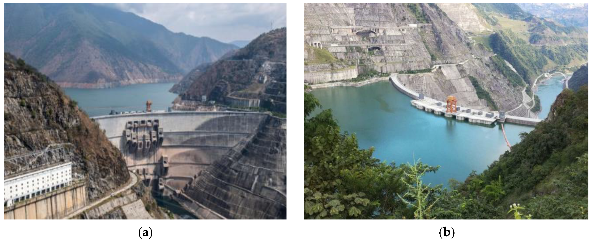
This case study explores an important hydropower project located in the middle reaches of the Lancang River in Yunnan Province. The project includes a series of infrastructures, including a concrete double-curvature arch dam, plunge pool, sub dam, spillway tunnel, and extensive underground water diversion power generation network. Among them, the Xiaowan double-curvature arch dam is the focus, with a dam height of 294.5 m, a standard water level of 1240 m, and an installed capacity of 4200 MW. It guarantees a capacity of 1778 megawatts (MW) and generates up to 1.9 million kWh (kWh) of electricity per year. The top view of the dam is shown in Figure 3.
The validity and accuracy of the dam deformation prediction model proposed in this paper are analyzed by using the monitoring data of A22-PL-02 and A22-PL-03 monitors of the Xiaowan double-curvature arch dam. This paper describes the advantages of the model in dam deformation analysis. In order to verify the reliability of the model, the monitoring data of arch crown beams A22-PL-02 and A22-PL-03 from December 2008 to December 2016 were used. The deformation prediction ability of the model was examined by 2896 sets of data sets. A total of 80% (2316 groups) of the data sets were allocated for model training, and the remaining 20% (580 groups) constituted the test set. The spatial distribution of arch dam measuring points is shown in Figure 4a, and the related environmental factors are shown in Figure 4b. These visual representations help in understanding the geospatial dynamics and environmental background of dam operation, thereby enhancing the robustness of deformation analysis.

5.1. Data Preprocessing: Constructing Model Feature Factors

In the process of collecting prototype data of dam deformation monitoring, a series of inevitable technical challenges are faced, including equipment dysfunction and data transmission failure, which lead to a small amount of missing data in the data set. For those partially missing monitoring data, this paper selects the cubic Hermite interpolation method for data supplement. The interpolation method can not only effectively restore the missing data but also maintain the local high-order continuity of the data, thus ensuring the integrity and accuracy of the data set and improving the reliability of subsequent analysis and model training. Based on the analysis of the influencing factors of dam deformation, the dam deformation displacement is composed of hydraulic component δH, temperature component δT, and aging component δθ [39].
{ δ H = i = 1 4 a 1 i ( H i H 0 i ) δ T = i = 1 2 [ b 1 i ( sin ( 2 π i t 365 ) sin ( 2 π i t 0 365 ) ) + b 2 i ( cos ( 2 π i t 365 ) cos ( 2 π i t 0 365 ) ) ] δ θ = c 1 ( θ θ 0 ) c 2 ( ln θ ln θ 0 )
The variables denoted by H and H0 represent the upstream water level and the base elevation of the dam, respectively, at the given moment; t and t0 represent the monitoring sequence at a specific moment and the reference moment, respectively; θ and θ0 are the ratios of t and t0 to 100, respectively; a1i, b1i, b2i, c1, and c2 correspond to the fitting coefficients. The resultant factor influencing water pressure is represented by H i H 0 i ( i = 1 , 2 , 3 , 4 ) . The temperature impact factor is sin ( 2 π i t 365 ) sin ( 2 π i t 0 365 ) , cos ( 2 π i t 365 ) cos ( 2 π i t 0 365 ) ( i = 1 , 2 ) . The aging influence factor is θθ0, lnθ − lnθ0.
In order to unify the range of different features to the same scale and reduce the numerical difference between features to avoid the negative impact on the accuracy of the model, data standardization has become a necessary preprocessing step.

5.2. Comparative Analysis of Decomposition and Reconstruction Techniques

In order to comprehensively evaluate the effectiveness of EMD, EEMD and CEEMDAN decomposition techniques in dam deformation monitoring data processing, a series of quantitative analysis was carried out. Specifically, in this paper, the EEMD and EMD algorithms are synchronized and applied to the standardized data set to facilitate the comparative evaluation of their error reconstruction capabilities. Through comparative analysis, it can be seen that the accuracy of EEMD reconstruction of dam deformation signal is significantly lower than that of traditional EMD method. This decline is largely attributed to the number of sets and white noise contained in EEMD. In contrast, the CEEMDAN algorithm shows stronger reconstruction performance. CEEMDAN shows a comparable error level with EMD, highlighting its advantages in signal reconstruction consistency. The results confirm that CEEMDAN improves the accuracy and efficiency of decomposition by noise cancellation. The reconstruction results of the three decomposition methods are shown in Figure 5.
Through the comparative analysis of the above three decomposition methods, it can be seen that CEEMDAN shows better performance. In practical engineering applications, this method has the following advantages: (1) The CEEMDAN method can extract features and trends from dam deformation data more accurately. The prediction model based on these reconstructed data has high accuracy and accuracy, which enhances the reliability and effectiveness of dam deformation prediction. (2) The safety management and maintenance of dams requires reliable engineering decisions, including maintenance planning, monitoring, and early warning systems. With the help of CEEMDAN, a more accurate deformation prediction model enhances the reliability of these decisions and improves the safety of the dam. (3) Dam monitoring and early warning systems rely on accurate data to identify potential anomalies and trigger timely interventions. The CEEMDAN decomposition provides more reliable and consistent data, thereby improving the performance of the monitoring and early warning system, reducing false positives and false negatives, and ensuring timely response to potential risks. (4) The CEEMDAN method enables dam managers to better formulate strategies and allocate resources by suppressing false positives and unnecessary maintenance tasks, thereby reducing costs and improving operational efficiency. (5) As an important infrastructure, the safety of the dam directly affects the stability and development of the surrounding areas. Using CEEMDAN to predict deformation is conducive to early detection of risks and taking preventive measures so as to ensure the development and stability of social economy.
The practical significance of the CEEMDAN reconstruction error being better than the other two is that (1) the prediction accuracy is improved, and the lower reconstruction error means that the IMFs extracted from the original signal are less different from the real signal; (2) the quality of signal analysis is improved, as CEEMDAN can more accurately reveal the trend, periodic components, and outliers in the dam deformation signal, which is helpful to better understand the dynamic process; and (3) by reducing the reconstruction error, CEEMDAN can reduce the false positives and omissions caused by the model prediction error to a certain extent.

5.3. Analysis of the Results of Sample Entropy and CEEMDAN

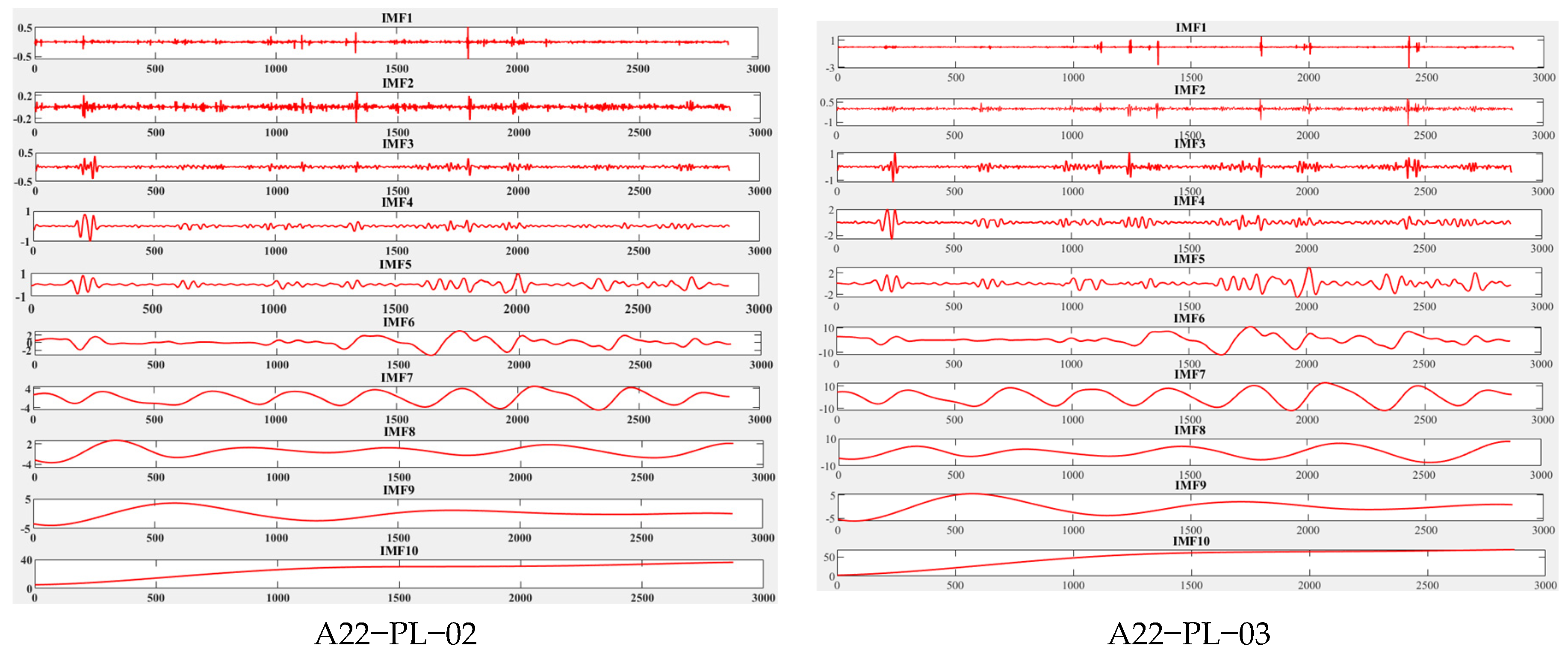
In the practical application of dam safety, it is a key work to use the CEEMDAN algorithm to decompose dam data, which is helpful to reveal the important features and patterns hidden in the data. The CEEMDAN algorithm decomposes the original dam data into multiple IMF components, and each IMF component represents the components of different frequencies and amplitudes in the data. When determining the key IMFs in these components, we usually compare them based on the sample entropy associated with each intrinsic IMF. Specifically, through the sample entropy analysis, the important IMFs in the dam data can be determined, which have significant fluctuations and characteristics in the data. In Figure 6, we can see the modal components after CEEMDAN-SE decomposition, which show different characteristics and fluctuation modes. It can be seen from Figure 7 that the sample entropy values of IMF1~IMF4 are higher than the overall data, so they represent high-frequency components with significant fluctuation characteristics. These high frequency components may be related to the subtle changes of the dam structure or the influence of environmental factors. IMF5~IMF7 show periodic oscillation, which may be related to the periodic change in dam stress or the influence of surrounding geological conditions. In contrast, IMF8~IMF10 are low frequency components, reflecting the time trend of dam deformation, which may be related to long-term structural changes or temperature and other factors.

5.4. The Final Model Input Variables Are Determined by PACF Analysis

In the practical application of dam safety, in order to improve the accuracy and effectiveness of the prediction model, the CEEMDAN-SE method is used to decompose the original time series data in detail to obtain 10 IMF components. These IMFs can capture the fluctuation characteristics of different scales in the original data and serve as signal sources for subsequent analysis.
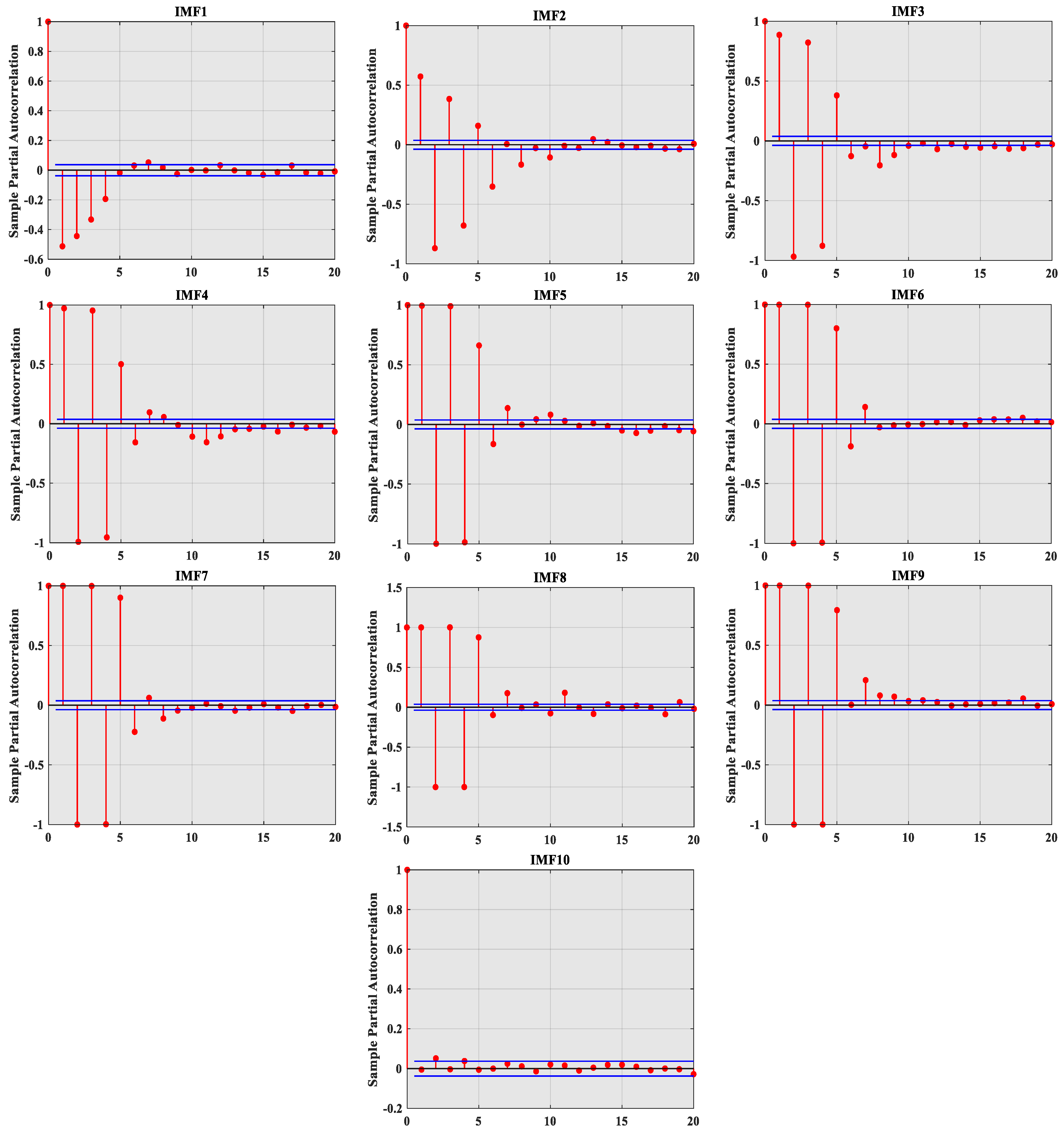
In this paper, PACF analysis is applied to the 10 IMF components generated above to quantify the direct relationship between time points in the time series and to eliminate the influence of indirect correlation in order to do an in-depth study of the correlation strength between its time series data points and select the best input feature set. As shown in Figure 8, by calculating the partial autocorrelation coefficient between the time series and its lag sequence, a significant correlation can be found, and the optimal input variable length of each GSWOA-KELM model can be determined. Table 1 provides a detailed configuration of the optimal input variables for each IMF component to ensure the maximum correlation between the input features and the target prediction output, thereby enhancing the prediction ability of the model. Through this method, we can make full use of the data after CEEMDAN-SE decomposition, combined with the GSWOA-KELM model and PACF analysis, to build a more accurate and reliable prediction model and provide more effective tools and means for dam safety management.
Selecting the appropriate input variables is the key to time series analysis and predictive modeling. The PACF results shown in Figure 8 provide an important statistical basis for variable selection. In this paper, taking IMF1 as an example, the maximum lag period with significant correlation is determined by identifying the PACF value initially exceeding the 95% confidence interval. Specifically, if this threshold is exceeded on the fifth day of the lag, it indicates that there is a significant linear correlation between the lag value from the first day to the fourth day and the current observation value. Based on this analysis, four consecutive lag values from (t − 4) to (t − 1) d are selected as input variables, where d represents the number of days and t represents the current time point. These variables are used to predict the target value of the current day (td). In addition, in order to evaluate the predictive ability of the model for dam operation and management from a broader perspective, this study extends the focus from predicting the current day (td) to predicting the next three days ((t + 3)d) and six days ((t + 6)d).
Figure 9 illustrates the selection of appropriate input variables for different prediction periods based on PACF results. This method framework provides systematic guidance for determining which historical data points are most predictive when constructing prediction models. This input variable selection strategy optimizes the prediction performance of the model and ensures the operation and management of the dam.

5.5. Selection of Kernel Functions and Comparative Analysis of GSWOA-KELM Models

In this paper, GSWOA-KELM is used to model and predict the two measuring points. The choice of kernel function in the KELM model plays an important role in its performance and behavior. The kernel function is used to map the input data to a high-dimensional space, thereby enhancing linear differentiability or promoting improved fitting in the above space. Different kernel functions produce different data mappings and model behaviors, which have different effects on model performance. Among all kernel functions, the linear kernel function operates by mapping the data to the original feature space without nonlinear transformation, making it suitable for linearly differentiable scenarios. Therefore, linear kernels show good performance on linearly differentiable data sets. In contrast, the radial basis function (RBF) kernel evaluates the similarity between points in the feature space by projecting the data into an infinite dimensional space and using the negative exponential distance from the data point to the center point. Although the RBF kernel usually performs well in dealing with nonlinear data, it needs to be cautious when tuning parameters, especially bandwidth parameters, to avoid overfitting. In addition, such as the Sigmoid kernel, it may produce good results in specific scenarios, although careful selection and adjustment are required based on existing problems. The selection of kernel function must consider data characteristics, problem complexity, and model performance requirements. Through the reasonable selection and adjustment of the kernel function, the generalization ability, fitting ability, and adaptability to new data of the model can be enhanced.
Therefore, in this paper, the prediction ability of the unoptimized KELM model is evaluated for the original dam deformation data set. Then, under the condition of the uniform data set shown in Figure 10a, the prediction performance of KELM models using different kernel functions is compared and evaluated, and the radar chart of the corresponding evaluation index is given in Figure 10b.
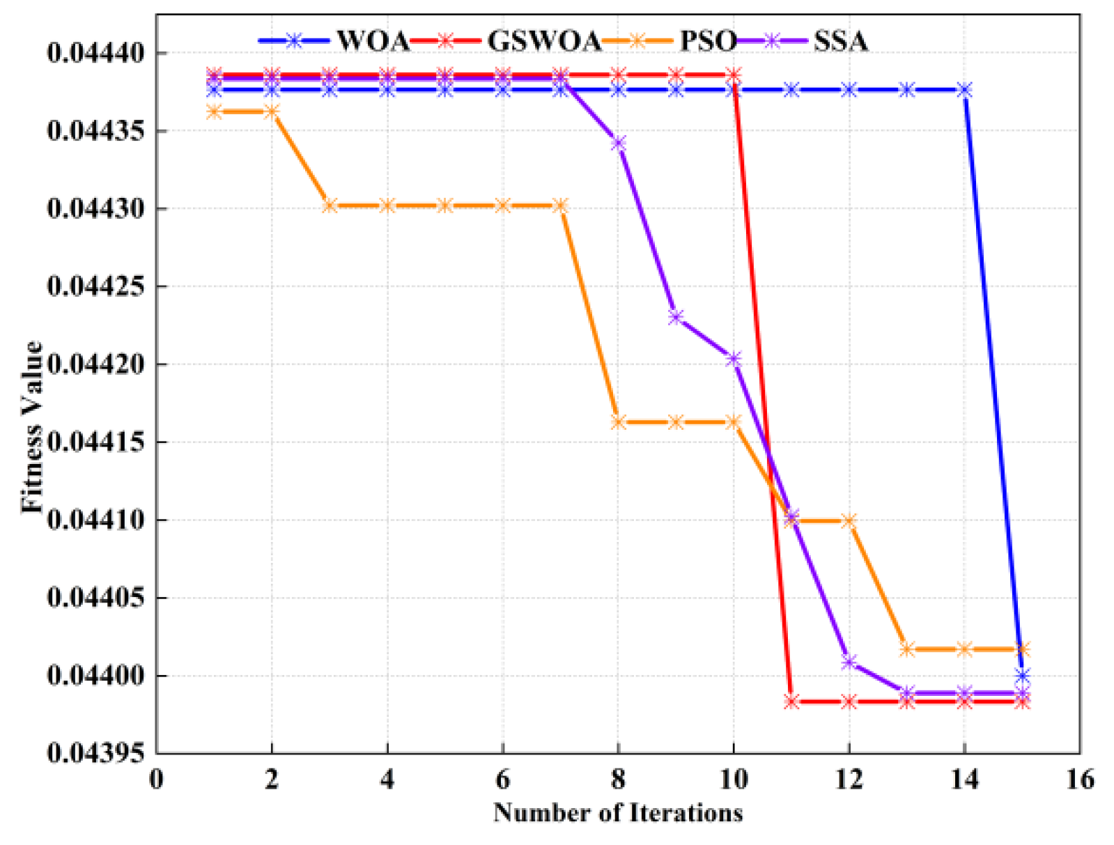
After determining the kernel function type, it is necessary to determine the regularization parameter (C), the kernel parameter, and the number of ELM hidden layer nodes. GSWOA has been widely used in the field of function optimization because of its fast computational efficiency, fast convergence speed, and strong global search ability. Therefore, this paper selects the GSWOA algorithm to optimize the KELM parameters. In this paper, GSWOA is compared with traditional algorithms to evaluate its adaptability. As shown in Figure 11, the convergence speed of GSWOA is significantly accelerated after the 10th iteration, which is a phenomenon that other algorithms have not observed in the same time. This observation shows that compared with other algorithms, GSWOA shows superior convergence speed and computational efficiency. The specific parameters of each algorithm are listed in Table 2.

5.6. Evaluate the Robustness and Computational Efficiency of the KELM Model

In the practical application of dam safety, in order to evaluate the prediction effect of the KELM model proposed in this paper, we choose the traditional BP, ELM, CNN, SVM, and GRU models as the comparison models. These models are used to predict dam deformation data using the same data set division as the model proposed in this paper, including training set and test set. At the same time, in order to ensure the consistency of the model, this paper uses the initial model to directly verify and compare all the models. This paper compares the prediction results of the models and evaluates their prediction performance through graph display and evaluation indicators. Figure 12 shows the prediction results of each model. By comparing the predicted values and measured values of different models, their fitting degree and prediction accuracy can be intuitively evaluated. By comparing the model proposed in this paper with the traditional neural network and machine learning model, its performance in dam deformation prediction can be comprehensively evaluated. Through this comparison, it is helpful to select the most suitable prediction model for practical application and provide a more reliable and effective prediction tool for dam safety management.
As shown in Figure 12, the KELM model, as the final prediction framework of this study, shows excellent prediction performance compared with the traditional model. See Table 3 for details. Compared with the BP model, the RMSE, MSE, and MAE of the KELM model are reduced by 0.1707 mm, 0.0882 mm2, and 0.1630 mm, respectively, while R2 is increased by 2.79%. Compared with the BP model, the advantages of the KELM model are as follows: (1) The KELM model has a faster training speed because it does not require an iterative back propagation algorithm to directly solve the output weight; (2) compared with the BP model, the KELM model requires fewer hyperparameters to adjust, which simplifies the implementation and adjustment process; and (3) the KELM model often avoids the problem of the BP model falling into the local optimum by randomly initializing the feature weights, thereby reducing the risk of falling into the local optimum.
Compared with the ELM model, the RMSE, MSE, and MAE of the KELM model are reduced by 0.8509 mm, 1.0185 mm2, and 0.8124 mm, respectively, and the R2 is increased by 31.87%. Compared with the ELM model, the advantages of the KELM model are as follows: (1) Compared with the ELM model, the KELM model usually requires less parameter optimization, which simplifies the model tuning process; (2) the KELM model shows enhanced robustness to the random weight initialization between the input layer and the hidden layer, ensuring continuous prediction performance stability; (3) the KELM model is usually easy to learn online and can quickly update and adjust when new data arrive.
Compared with the CNN, SVM, and GRU models, the KELM model has a significant improvement in all evaluation indicators. Therefore, by predicting the dam deformation at different measuring points, this paper confirms the general effectiveness of the proposed model and also confirms its robustness to predict dam deformation skillfully even in the case of partial missing original data.
In order to verify the computational efficiency advantage of the model proposed in this study, we recorded the average execution time of 20 independent runs of each model, which is recorded separately in Table 4. It can be seen from Table 4 that the CNN and GRU models require longer running time when applied to the same target sequence. This difference is due to the fact that CNN often requires additional convolutional layers and filters to extract relevant features, which increases the complexity of the model. GRU performs well in retaining long-term dependent information in time series data. Compared with the CNN and GRU models, the KELM model shows higher computational efficiency. This observation shows that (1) the KELM model usually requires less memory resources because it does not need to store a large number of convolution kernel parameters. Therefore, it performs well in terms of parameter storage efficiency and computational cost benefits. (2) The KELM model has fewer parameters and a relatively simple structure, which enhances the interpretability and comprehensibility of the prediction process. (3) The KELM model shows greater flexibility in dealing with unstructured and sequential data, making it suitable for different data models.

5.7. Deformation Prediction Results and Comparative Analysis

In the practical application of dam safety, in order to verify the effectiveness of the proposed dam deformation monitoring model, it is compared with the CEEMDAN-WOA-KELM, GSWOA-KELM, CEEMDAN-KELM, and KELM models. These models represent different methods and strategies, and we compare them with the proposed models to evaluate their predictive performance. Firstly, the dam deformation data of each model are predicted, and the prediction results are compared. In this paper, the positive vertical lateral displacement is selected for the A22-PL-02 measuring point, and the positive vertical longitudinal displacement is selected for the A22-PL-03 measuring point: (1) There are significant differences in the structure and stress state of the dam at different locations. Some measuring points are susceptible to lateral forces, while others are mainly affected by vertical forces. Therefore, monitoring the displacement in different directions is helpful to fully understand the deformation behavior of the dam. (2) In the dam deformation monitoring, the key parts need to focus on the horizontal or vertical displacement to prevent the risk of structural instability or settlement. According to the location and importance, it is necessary to select the appropriate displacement direction for prediction. (3) The characteristics of displacement data in different directions may affect the prediction performance of the model. By analyzing historical data and selecting displacement prediction in a specific direction, the accuracy and reliability of the model can be improved.
Figure 13 shows the prediction results of each model. By comparing the predicted values of different models with the actual observations, the fitting degree and prediction accuracy can be evaluated. At the same time, we also analyze the residuals of each model. Figure 14 shows the residual distribution of each model. The final prediction results are shown in Table 5. These indicators can objectively evaluate the prediction accuracy and goodness of fit of the model and help us determine which model performs best in dam deformation analysis. Through comparative analysis, the optimal dam deformation analysis model can be determined, and its effectiveness in practical application can be verified.
It can be seen from Figure 13 that the prediction performance of the CEEMDAN-SE-PACF-GSWOA-KELM model is better than that of the CEEMDAN-WOA-KELM, GSWOA-KELM, CEEMDAN-KELM, and KELM models to varying degrees. The A22-PL-02 measurement points in Table 5 are analyzed. Compared with the CEEMDAN-WOA-KELM model, RMSE, MSE, and MAE are reduced by 0.5992 mm, 1.1303 mm2, and 0.5523 mm, respectively, and R2 is increased by 6.83%. This shows that the GSWOA algorithm is effective in optimizing the key parameters of KELM, and the prediction accuracy of the model is improved compared with the WOA. Specifically, 1. GSWOA introduces the variable spiral position update, which improves the global search diversity and the ability of the algorithm to find the optimal solution; 2. GSWOA enhances the search stability, reduces the risk of falling into local optimum, and improves the robustness of the algorithm; and 3. GSWOA shows adaptability to different optimization problems and shows stronger generalization ability in complex scenes.
Compared with the GSWOA-KELM model, the RMSE, MSE, and MAE of the CEEMDAN-SE-PACF-GSWOA-KELM model are reduced by 0.3340 mm, 0.5414 mm2, and 0.3702 mm, respectively, while R2 is increased by 4.79%. This shows that the advantages of CEEMDAN-SE-PACF preprocessing are as follows: (1) CEEMDAN-SE-PACF effectively extracts the principal components of the signal, filters out the noise data components, and improves the data quality and accuracy; (2) CEEMDAN-SE-PACF identifies key signal features, which helps to understand the inherent laws of data and improve prediction accuracy; and (3) CEEMDAN-SE-PACF performs downscaling processing on the signal, reduces the data complexity, improves the analysis efficiency, and reduces the risk of overfitting.
Compared with the CEEMDAN-KELM model, the RMSE, MSE, and MAE of the CEEMDAN-SE-PACF-GSWOA-KELM model are reduced by 1.2763 mm, 3.3046 mm2, and 1.1409 mm, respectively, and R2 is increased by 14.37%. This emphasizes both the benefits of algorithm optimization and the benefits of data preprocessing.
The following can be seen from Figure 14: (1) From the residual diagram, it can be seen that the CEEMDAN-SE-PACF-GSWOA-KELM model obeys the normal distribution, while other models show different degrees of bell symmetry, indicating that it approximately obeys the normal distribution. (2) For the CEEMDAN-SE-PACF-GSWOA-KELM model, the residual mean tends to zero, indicating that the deviation is the smallest, and the deviation from zero means that other models have potential model deviations. (3) It is worth noting that the abnormal residual distribution of the CEEMDAN-WOA-KELM, GSWOA-KELM, CEEMDAN-KELM, and KELM models indicates the prediction bias or error in some scenarios.

6. Conclusions

Aiming at the data noise and nonlinear characteristics, this paper uses the complete ensemble empirical mode decomposition with adaptive noise (CEEMDAN) method to improve the decomposition accuracy of the initial deformation sequence by introducing the white noise of Gaussian distribution. Then, the sample entropy (SE) is used to evaluate the complexity of each intrinsic mode function (IMF) obtained by decomposition, and the sample entropy of the initial data is used as the reference standard to properly reconstruct these modal components. In addition, partial autocorrelation function (PACF) analysis is used to identify the best correlation features between a single IMF and past data. Then, these identified features are used to construct input feature vectors for GSWOA-KELM to enhance the prediction performance of the model. In addition, the data of the Xiaowan double-curvature arch dam are used to verify the analysis. Using various indicators to evaluate the performance of the model, the following conclusions are drawn:
(1)
The CEEMDAN-SE-PACF-GSWOA-KELM model proposed in this paper has higher prediction accuracy than other models. In order to solve the nonlinear characteristics of the original data of the dam, this paper compares the CEEMDAN and EEMD methods and uses the reconstruction error and signal-to-noise ratio index. The results show that the CEEMDAN decomposition method is superior to EEMD in accurately decomposing dam signals, thereby improving the reliability of engineering decision-making in practical applications.
(2)
Effective management and maintenance of dams require reliable engineering decisions, including robust maintenance plans and monitoring strategies. In order to improve the accuracy of CEEMDAN decomposition, in this paper, SE and PACF are integrated into the CEEMDAN decomposition process, which is beneficial to filter noise more effectively and improve the quality of decomposition results. In addition, SE and PACF methods help to identify prominent signal features, thereby identifying and capturing key components and trends in the signal. Through the analysis of sample entropy and autocorrelation function, the frequency components and time series characteristics of the signal can be accurately determined so as to provide a more reliable basis for subsequent analysis and modeling work.
(3)
In order to construct a more effective prediction model, the GSWOA algorithm is used to optimize the parameters of the KELM model. At the same time, the effectiveness of the GSWOA algorithm is compared with the traditional algorithm, and the superior convergence characteristics of the GSWOA algorithm are revealed. In addition, in the final prediction comparison analysis, the prediction performance of the WOA-KELM and GSWOA-KELM models is juxtaposed, which shows the ability of the GSWOA algorithm to optimize the parameters of the KELM model and obtains better prediction results.
(4)
This paper aims to verify the robustness and computational efficiency of the KELM model by comparing it with several traditional prediction models. Through comparative analysis, the advantages of the KELM model are summarized as follows: a. Compared with the BP model, the KELM model usually avoids the local optimal problem by randomly initializing the feature weights, thereby reducing the possibility of converging to the suboptimal solution. b. Compared with the ELM model, the KELM model shows greater flexibility in random weight initialization between the input layer and the hidden layer, ensuring more consistent prediction performance. c. Compared with the SVM model, the KELM model has higher efficiency in dealing with high-dimensional data, because it does not need to explicitly calculate the kernel function or construct the kernel matrix. Therefore, compared with other traditional models, the robustness and computational efficiency of the KELM model have been verified to varying degrees.

Author Contributions

Conceptualization, B.Z. and B.O.; validation, Z.W., S.F. and D.C.; writing-original draft preparation, Z.W. and L.G.; methodology, B.Z. and T.Y.; funding, B.O., Z.W. and D.Z.; All authors have read and agreed to the published version of the manuscript.

Funding

This work was supported by National Natural Science Foundation of China [Grant Nos. 52069029, 52369026]; the Yunnan Key Laboratory of Water Conservancy and Hydropower Engineering Safety [Grant No. 202302AN360003]; and the Yunnan Province Agricultural Basic Research Joint Special General Project [Grant No. 202401BD070001-071].

Data Availability Statement

Original date is available upon reasonable request.

Conflicts of Interest

Author Bin Zhou was employed by the Yunnan Infrastructure Investment Co., Ltd. The remaining authors declare that the research was conducted in the absence of any commercial or financial relationships that could be construed as a potential conflict of interest.

References

  1. Gu, C.; Su, H.; Liu, H. Review of Research on Risk Analysis and Management of Dam Service. J. Water Resour. 2018, 49, 26–35. [Google Scholar] [CrossRef]
  2. Wu, Z. Theory and Method of Dam and Dam Foundation Safety Monitoring and Its Application. Jiangsu Sci. Technol. Inform. 2005, 12, 1–6. [Google Scholar]
  3. Huang, S. Analysis of Dam Deformation Monitoring Based on Statistical-Stepwise Regression Model. Water Resour. Sci. Econ. 2023, 29, 1–8. [Google Scholar]
  4. Su, H.; Li, X.; Yang, B.; Wen, Z. Wavelet Support Vector Machine-Based Prediction Model of Dam Deformation. Mech. Syst. Signal Process. 2018, 110, 412–427. [Google Scholar] [CrossRef]
  5. Xing, Y.; Chen, Y.; Huang, S.; Wang, P.; Xiang, Y. Research on Dam Deformation Prediction Model Based on Optimized SVM. Processes 2022, 10, 1842. [Google Scholar] [CrossRef]
  6. Ren, Q.; Li, M.; Song, L.; Liu, H. An Optimized Combination Prediction Model for Concrete Dam Deformation Considering Quantitative Evaluation and Hysteresis Correction. Adv. Eng. Inform. 2020, 46, 101154. [Google Scholar] [CrossRef]
  7. Wei, B.; Chen, L.; Li, H.; Yuan, D.; Wang, G. Optimized Prediction Model for Concrete Dam Displacement Based on Signal Residual Amendment. Appl. Math. Modell. 2020, 78, 20–36. [Google Scholar] [CrossRef]
  8. Dai, B.; Gu, H.; Zhu, Y.; Chen, S.; Rodriguez, E.F. On the Use of an Improved Artificial Fish Swarm Algorithm-Backpropagation Neural Network for Predicting Dam Deformation Behavior. Complexity 2020, 2020, 5463893. [Google Scholar] [CrossRef]
  9. Kang, F.; Liu, J.; Li, J.; Li, S. Concrete Dam Deformation Prediction Model for Health Monitoring Based on Extreme Learning Machine. Struct. Control Health Monit. 2017, 24, e1997. [Google Scholar] [CrossRef]
  10. Zhang, Y.; Zhang, W.; Li, Y.; Wen, L.; Sun, X. AF-OS-ELM-MVE: A New Online Sequential Extreme Learning Machine of Dam Safety Monitoring Model for Structure Deformation Estimation. Adv. Eng. Inform. 2024, 60, 102345. [Google Scholar] [CrossRef]
  11. Cao, E.; Bao, T.; Liu, Y.; Li, H.; Yuan, R.; Hu, S. A Data Enhancement-Based Quadratic Imputation Framework for Consecutive Missing Values Considering Spatiotemporal Characteristics of Dam Deformation. J. Civ. Struct. Health Monit. 2024, 14, 431–447. [Google Scholar] [CrossRef]
  12. Ou, B.; Wu, B.; Yuan, J.; Li, S. Concrete Dam Deformation Prediction Model Based on LSTM. Adv. Water Resour. Hydropower Sci. Technol. 2022, 42, 21–26. [Google Scholar]
  13. Cai, S.; Gao, H.; Zhang, J.; Peng, M. A Self-Attention-LSTM Method for Dam Deformation Prediction Based on CEEMDAN Optimization. Appl. Soft Comput. 2024, 159, 111615. [Google Scholar] [CrossRef]
  14. Cao, E.; Bao, T.; Yuan, R.; Hu, S. Hierarchical Prediction of Dam Deformation Based on Hybrid Temporal Network and Load-Oriented Residual Correction. Eng. Struct. 2024, 308, 117949. [Google Scholar] [CrossRef]
  15. Zhang, C.; Fu, S.; Ou, B.; Liu, Z.; Hu, M. Prediction of Dam Deformation Using SSA-LSTM Model Based on Empirical Mode Decomposition Method and Wavelet Threshold Noise Reduction. Water 2022, 14, 3380. [Google Scholar] [CrossRef]
  16. Wei, Y.; Li, Q.; Hu, Y.; Wang, Y.; Zhu, X.; Tan, Y.; Liu, C.; Pei, L. Deformation Prediction Model Based on an Improved CNN + LSTM Model for the First Impoundment of Super-High Arch Dams. J. Civil Struct. Health Monit. 2023, 13, 431–442. [Google Scholar] [CrossRef]
  17. Zhang, S.; Zheng, D.; Liu, Y. Deformation Prediction System of Concrete Dam Based on IVM-SCSO-RF. Water 2022, 14, 3739. [Google Scholar] [CrossRef]
  18. Liu, M.; Wen, Z.; Zhou, R.; Su, H. Bayesian Optimization and Ensemble Learning Algorithm Combined Method for Deformation Prediction of Concrete Dam. Structures 2023, 54, 981–993. [Google Scholar] [CrossRef]
  19. Lin, C.; Zou, Y.; Lai, X.; Wang, X.; Su, Y. Variation Trend Prediction of Dam Displacement in the Short-Term Using a Hybrid Model Based on Clustering Methods. Appl. Sci. 2023, 13, 10827. [Google Scholar] [CrossRef]
  20. Xu, B.; Chen, Z.; Wang, X.; Bu, J.; Zhu, Z.; Zhang, H.; Wang, S.; Lu, J. Combined Prediction Model of Concrete Arch Dam Displacement Based on Cluster Analysis Considering Signal Residual Correction. Mech. Syst. Signal Process. 2023, 203, 110721. [Google Scholar] [CrossRef]
  21. Tang, Y.; Yang, M.; Li, B.; Guo, J.; Chen, Y. A Two-Stage Dam Deformation Prediction Model Based on Deep Learning. China’s Rural. Water Conserv. Hydropower 2024, 16, 225–230+237. [Google Scholar]
  22. Cao, E.; Bao, T.; Gu, C.; Li, H.; Liu, Y.; Hu, S. A Novel Hybrid Decomposition—Ensemble Prediction Model for Dam Deformation. Appl. Sci. 2020, 10, 5700. [Google Scholar] [CrossRef]
  23. Jiang, P.; Qi, H.; Li, T. Application of IF-KELM Model in Deformation Prediction of Concrete Arch Dam. Hydropower 2023, 49, 96–100. [Google Scholar]
  24. Zhou, L.; Xu, C.; Yuan, Z.; Lu, T. Dam Deformation Prediction Based on CEEMDAN-PSR-KELM. Peoples Yellow River 2019, 41, 138–141+145. [Google Scholar] [CrossRef]
  25. Xu, G.; Lu, Y.; Jing, Z.; Wu, C.; Zhang, Q. IEALL: Dam Deformation Prediction Model Based on Combination Model Method. Appl. Sci. 2023, 13, 5160. [Google Scholar] [CrossRef]
  26. Wu, Z.H.; Huang, N.E. Ensemble Empirical Mode Decomposition: A Noise Assisted Data Analysis Method. Adv. Adapt. Data Anal. 2009, 1, 1–41. [Google Scholar] [CrossRef]
  27. Torres, M.E.; Colominas, M.A.; Schlotthauer, G.; Flandrin, P. A Complete Ensemble Empirical Mode Decomposition with Adaptive Noise. In Proceedings of the 2011 IEEE International Conference on Acoustics, Speech, and Signal Processing (ICASSP), Prague, Czech Republic, 22–27 May 2011. [Google Scholar]
  28. Qin, Z.; Chen, H.; Chang, J. Signal-to-Noise Ratio Enhancement Based on Empirical Mode Decomposition in Phase-Sensitive Optical Time Domain Reflectometry Systems. Sensors 2017, 17, 1870. [Google Scholar] [CrossRef]
  29. Dang, J.; Li, J.; Jia, R.; Fan, P. Noise Reduction of Hydropower Unit Vibration Signals Based on EMD Continuous Geometric Distribution. J. Hydropower Gener. 2020, 39, 46–54. [Google Scholar] [CrossRef]
  30. Zhao, H.; Hua, H.; Wang, H.; Yue, Y. Short-Term Wind Power Interval Prediction Based on LCD-SE-IWOA-KELM. Electr. Meas. Instrum. 2020, 57, 77–83. [Google Scholar] [CrossRef]
  31. Richman, J.S.; Moorman, J.R. Physiological Time-Series Analysis Using Approximate Entropy and Sample Entropy. Am. J. Physiol. 2000, 278, H2039–H2049. [Google Scholar] [CrossRef]
  32. Weiß, C.H.; Aleksandrov, B.; Faymonville, M.; Jentsch, C. Partial Autocorrelation Diagnostics for Count Time Series. Entropy 2023, 25, 105. [Google Scholar] [CrossRef] [PubMed]
  33. Liu, M.; Wen, Z.; Su, H. Deformation Prediction Based on Denoising Techniques and Ensemble Learning Algorithms for Concrete Dams. Expert Syst. Appl. 2024, 238 Pt C, 122022. [Google Scholar] [CrossRef]
  34. Mirjalili, S.; Lewis, A. The Whale Optimization Algorithm. Adv. Eng. Softw. 2016, 95, 51–67. [Google Scholar] [CrossRef]
  35. Oliva, D.; Abd El Aziz, M.; Hassanien, A.E. Parameter Estimation of Photovoltaic Cells Using an Improved Chaotic Whale Optimization Algorithm. Appl. Energy 2017, 200, 141–154. [Google Scholar] [CrossRef]
  36. Liu, L.; Bai, K.; Dan, Z.; Zhang, S.; Liu, Z. A Whale Optimization Algorithm for Global Search Strategy. Small Microcomput. Syst. 2020, 41, 1820–1825. [Google Scholar]
  37. Yang, T.; Li, W.; Huang, Z.; Peng, L.; Yang, J. Short-Term Prediction of Wind Power Generation Based on VMD-GSWOA-LSTM Model. AIP Adv. 2023, 13, 085215. [Google Scholar] [CrossRef]
  38. Liu, X.; Kang, F.; Ma, C.; Li, H. Concrete Arch Dam Behavior Prediction Using Kernel-Extreme Learning Machines Considering Thermal Effect. J. Civil Struct. Health Monit. 2021, 11, 283–299. [Google Scholar] [CrossRef]
  39. Ou, B.; Zhang, C.; Xu, B.; Fu, S.; Liu, Z.; Wang, K. Innovative Approach to Dam Deformation Analysis: Integration of VMD, Fractal Theory, and WOA-DELM. Struct. Control Health Monit. 2024, 1710019. [Google Scholar] [CrossRef]
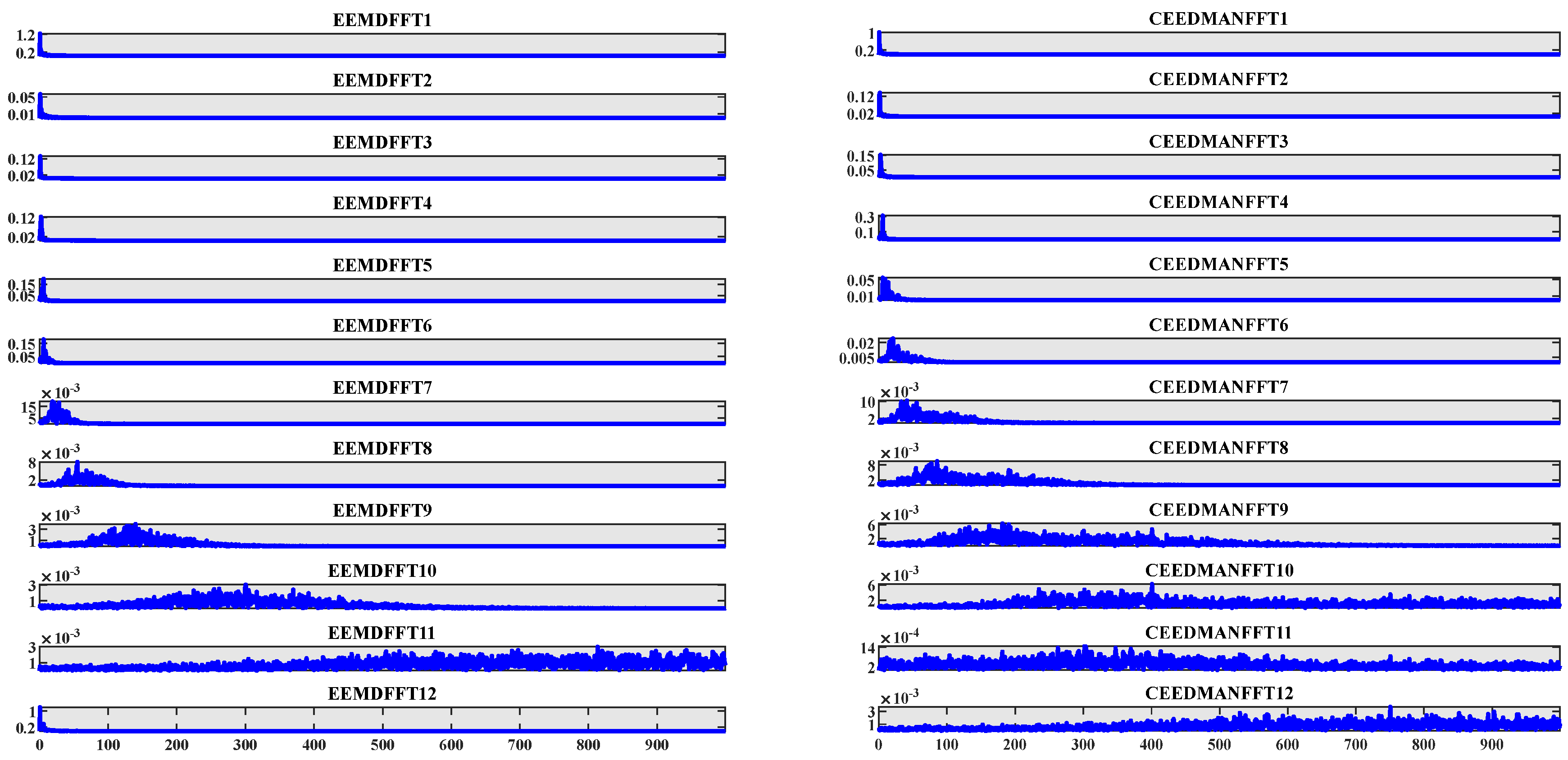
Figure 1. Comparison of CEEMDAN and EEMD decomposition results.
Water 16 01766 g001
Figure 2. Predictive model for dam deformation analysis.
Water 16 01766 g002
Figure 3. Aerial view of the dam. (a) Downstream view; (b) Upstream view.
Water 16 01766 g003
Figure 4. Layout of dam drape monitoring instrumentation. (a) Distribution of arch dam measurement points; (b) Chart of changes in environmental quantities.
Water 16 01766 g004
Figure 5. Reconstruction error diagram for each decomposition method.
Water 16 01766 g005
Figure 6. CEEMDAN decomposition results.
Water 16 01766 g006
Figure 7. Sample entropy value.
Water 16 01766 g007
Figure 8. PACF values for each IMF component.
Water 16 01766 g008
Figure 9. The process of determining the input and output variables of the IMF.
Water 16 01766 g009
Figure 10. Comparative Chart of KELM Prediction Results Using Different Kernel Functions and Performance Metrics Radar Chart. (a) Predictions Comparing Kernel Functions; (b) Radar Chart of Evaluation Indicators.
Water 16 01766 g010
Figure 11. Fitness Comparison Curves between GSWOA and Traditional Models.
Water 16 01766 g011
Figure 12. Comparative Prediction Model Results Graph.
Water 16 01766 g012
Figure 13. Modeling Results Graph.
Water 16 01766 g013
Figure 14. Residuals of Model Predictions.
Water 16 01766 g014
Table 1. Input variables for each IMF.
Modal ComponentNumber of InputsInput Variable
IMF14 x t 1 , x t 2 , x t 3 , x t 4
IMF28 x t 1 , x t 2 , x t 3 , x t 4 , x t 5 , x t 6 , x t 8 , x t 10
IMF37 x t 1 , x t 2 , x t 3 , x t 4 , x t 5 , x t 6 , x t 8
IMF410 x t 1 , x t 2 , x t 3 , x t 4 , x t 5 , x t 6 , x t 7 , x t 10 , x t 11 , x t 12
IMF57 x t 1 , x t 2 , x t 3 , x t 4 , x t 5 , x t 6 , x t 7
IMF67 x t 1 , x t 2 , x t 3 , x t 4 , x t 5 , x t 6 , x t 7
IMF78 x t 1 , x t 2 , x t 3 , x t 4 , x t 5 , x t 6 , x t 7 , x t 8
IMF88 x t 1 , x t 2 , x t 3 , x t 4 , x t 5 , x t 6 , x t 7 , x t 11
IMF96 x t 1 , x t 2 , x t 3 , x t 4 , x t 5 , x t 7
IMF101 x t 2
Table 2. Specific parameter settings of each algorithm.
algorithm parametersGSWOAWOAPSOSSA
whale population = 15whale population = 15Population size = 15population size = 15
dimensional = 2dimensional = 2inertia weight w = 0.8proportion of investigators = 20%
lower limit LB = [0, 1]lower limit LB = [0, 1]iteration speed range = [−5 × 10², 5 × 10²]percentage of discoverers = 70%
upper limit UB = [1, 1000]upper limit UB = [1, 1000]study factor c1, c2 = 1.5proportion of participants = 10%
iterations MaxI = 15iterations MaxI = 15iterations MaxI = 15iterations MaxI = 15
Table 3. Error Indices of Comparative Methods.
ModelRMSE/mmMSE/mm2R2MAE/mm
KELM0.17300.02990.99050.1243
BP0.34370.11810.96260.2873
ELM1.02391.04840.67180.9367
CNN0.60730.36880.88180.4216
SVM0.65430.41640.86970.5743
GRU0.94790.89860.64670.8179
Table 4. Comparison of calculation efficiency of each model.
ModelAverage Execution Time/s
KELM4.31
BP9.45
ELM10.01
CNN58.72
SVM6.45
GRU50.87
Table 5. Error indicators for different combination methods.
Monitoring PointModelRMSE/mmMSE/mm2R2MAE/mm
A22-PL-02CEEMDAN-SE-PACF-GSWOA-KELM0.64370.41440.99700.4476
CEEMDAN-WOA-KELM1.24291.54470.92870.9999
GSWOA-KELM0.97770.95580.94910.8178
CEEMDAN-KELM1.92853.71900.85331.5885
KELM1.04721.09670.93210.8684
A22-PL-03CEEMDAN-SE-PACF-GSWOA-KELM0.04270.00180.93340.0288
CEEMDAN-WOA-KELM0.05880.00310.91310.0303
GSWOA-KELM0.06990.00490.86380.0561
CEEMDAN-KELM0.06280.00430.81950.0502
KELM0.07170.00510.85680.0644
Disclaimer/Publisher’s Note: The statements, opinions and data contained in all publications are solely those of the individual author(s) and contributor(s) and not of MDPI and/or the editor(s). MDPI and/or the editor(s) disclaim responsibility for any injury to people or property resulting from any ideas, methods, instructions or products referred to in the content.