Article

Water Flow Prediction Based on Improved Spatiotemporal Attention Mechanism of Long Short-Term Memory Network

1
College of Information and Communication Engineering, Beijing University of Technology, Beijing 100124, China
2
Beijing South-North Water Diversion Tuancheng Lake Management Office, Beijing 100097, China
*
Author to whom correspondence should be addressed.
Water 2024, 16(11), 1600; https://doi.org/10.3390/w16111600
Submission received: 28 April 2024 / Revised: 29 May 2024 / Accepted: 30 May 2024 / Published: 3 June 2024

Abstract

:
The prediction of water plant flow should establish relationships between upstream and downstream hydrological stations, which is crucial for the early detection of flow anomalies. Long Short-Term Memory Networks (LSTMs) have been widely applied in hydrological time series forecasting. However, due to the highly nonlinear and dynamic nature of hydrological time series, as well as the intertwined coupling of data between multiple hydrological stations, the original LSTM models fail to simultaneously consider the spatiotemporal correlations among input sequences for flow prediction. To address this issue, we propose a novel flow prediction method based on the Spatiotemporal Attention LSTM (STA-LSTM) model. This model, based on an encoder–decoder architecture, integrates spatial attention mechanisms in the encoder to adaptively capture hydrological variables relevant to prediction. The decoder combines temporal attention mechanisms to better propagate gradient information and dynamically discover key encoder hidden states from all time steps within a window. Additionally, we construct an extended dataset, which preprocesses meteorological data with forward filling and rainfall encoding, and combines hydrological data from multiple neighboring pumping stations with external meteorological data to enhance the modeling capability of spatiotemporal relationships. In this paper, the actual production data of pumping stations and water plants along the East-to-West Water Diversion Project are taken as examples to verify the effectiveness of the model. Experimental results demonstrate that our STA-LSTM model can better capture spatiotemporal relationships, yielding improved prediction performance with a mean absolute error (MAE) of 3.57, a root mean square error (RMSE) of 4.61, and a mean absolute percentage error (MAPE) of 0.001. Additionally, our model achieved a 3.96% increase in R2 compared to the baseline model.

1. Introduction

An essential aspect of urban water resource management [1] is the prediction of pipeline flow in water treatment plants, which plays a crucial role in formulating policies such as water resource allocation, reservoir operation, flood prevention measures, and drought relief strategies. Accurately predicting pipeline flow not only helps optimize the use of water resources but also ensures downstream demand, flood prevention, and promotes water balance in reservoir operation [1,2].
Traditional hydrological forecasting methods rely on researchers’ in-depth understanding of water resource management and hydrological knowledge [3,4]. These methods require combining hydraulic process mathematical models with computer simulation techniques and mathematical equations to numerically simulate water conveyance systems [5,6]. However, such methods are limited by the difficulty of manual modeling and fixed engineering physical models [7] and boundary conditions, resulting in poor usability and accuracy. The introduction of machine learning methods has brought new perspectives to flow prediction tasks [8,9]. Since machine learning models learn the complex relationships of systems based on historical data without relying on prior engineering physical models, they help overcome problems caused by imperfect or inaccurate engineering models [10,11,12]. Farshed Fathian analyzed the stochastic and deterministic components of data time series and constructed a hybrid model RF-SETAR to forecast river flow [13]. Ahmad Khazaee Poul combined methods such as MLR, ANN, ANFIS, and KNN with wavelet transform [14] to improve the accuracy of monthly flow forecasts for the St. Clair River. Although there are some achievements for machine learning methods and their improved algorithms in the field of water flow prediction, their ability to extract and process multidimensional features still needs improvement [15].
The introduction of deep learning methods can effectively utilize multidimensional data. The Recurrent Neural Networks (RNNs) proposed by Zaremba et al. [16] have shown significant advantages in terms of time complexity and accuracy. Zhou et al. [17] improved the RNN with Unscented Kalman Filtering post-processing to predict the inflow sequence of the Three Gorges Reservoir in China. However, the increasing difficulty of data fitting and the increase in the number of network layers often lead to the problems of vanishing gradients and exploding gradients during the optimization process. The emergence of Long Short-Term Memory Networks (LSTMs) [18] effectively alleviates these issues and demonstrates more powerful capabilities in time series analysis tasks. Le’s study in 2019 indicated that the ability of LSTM in watershed hydrological modeling has been confirmed in multiple fields such as river flow and flood prediction [19]. Hu et al. utilized an LSTM deep learning model to predict the runoff data of the Tunxi hydrological station for the next six hours [20]. Compared to Support Vector Regression (SVR) and Multilayer Perceptron (MLP) models, LSTM exhibited superior performance. Although LSTM is very helpful in capturing long-term dependencies, it cannot focus on different variables at different time steps. To overcome these challenges, an attention-based encoder–decoder network was proposed in [21]. It converts the input sequence into a fixed-length vector through the encoder part [22], which is then converted into an output sequence by the decoder.
Although the deep learning method LSTM performs well in hydrological prediction models, the current research still faces two challenges in practical applications [23,24]. Firstly, flow prediction tasks are often not only directly related to upstream flow, but also to various factors such as geographical location, environmental conditions, and weather [25]. Studies have shown that models based on spatial and temporal features have better predictive capabilities [26,27,28,29]. Wang et al. accurately predicted the water level of the Hanjiang River using an LSTM network augmented with the spatiotemporal attention mechanism [30]. Li et al. utilize a spatiotemporal enhanced network for predicting machine Remaining Useful Life [31]. The lack of ability to capture spatiotemporal features in the prediction model limits the accuracy of the flow prediction task and the adaptability to dynamic scenes [32,33]. Secondly, deep learning models often lack intuitive interpretability [34,35]. Although LSTM has good accuracy in predicting flow data over time, the inability to verify the predicted results hinders the practical application of deep learning methods [36,37].
To address the two challenges mentioned earlier and capture key information from multidimensional spatiotemporal input attributes relevant to flow prediction objectives, this paper introduces an improved spatiotemporal attention mechanism on top of the standard LSTM network. Our research innovatively utilizes data from upstream and downstream pumping stations to predict current pump station flows, rather than relying solely on the physical parameters of the current station. By leveraging data from multiple geographic locations, STA-LSTM captures complex spatiotemporal relationships that traditional models often ignore. In addition, the attention mechanism provides a visual representation of the attention score, which can provide a deeper understanding of the model’s decision-making process and further promote the model’s application in the real world.
The architecture of this model consists of two main parts: the encoder and the decoder. The encoder consists of a spatial attention mechanism module based on LSTM units, which can adaptively identify and capture important spatial attributes closely related to the prediction target at each time step. The decoder contains another set of LSTM unit-based time attention mechanism modules, whose main function is to dynamically identify key hidden states related to the prediction target in all time steps within the window. With the help of the attention mechanism, the STA-LSTM model can not only adaptively select input spatial attributes most relevant to the prediction but also detect long-term dependencies in the time series. The method is validated using actual data from the East-to-West Water Diversion Project in Beijing, demonstrating the effectiveness and prediction accuracy of the approach.
The main work of this study can be summarized as follows:
  • Integration of LSTM with Spatiotemporal Attention Mechanism: Construct a water plant pipeline flow prediction model that combines Long Short-Term Memory (LSTM) networks with spatiotemporal attention mechanisms, improving the model’s interpretability of flow changes. Achieve the visual representations of spatial and temporal attention weights, and preliminarily explain their relationship with hydrological prediction.
  • Fusion of Hydrological Station Parameters and Meteorological Conditions: Innovatively utilize surrounding hydrological station parameters in conjunction with external meteorological conditions for water plant flow prediction and to improve prediction accuracy.
The structure of the article is as follows: Section 2 provides a detailed description of the construction of the dataset, the preprocessing process, and the formulation of flow prediction task objectives. Section 3 specifically introduces the STA-LSTM model, including the design of the backbone LSTM model and the spatiotemporal attention mechanism. Section 4 elaborates on the experimental part, including the settings of the experimental environment, experimental results, and analysis. Finally, Section 5 summarizes the research findings and proposes prospects for future work.

2. Materials

2.1. Study Area

The East-to-West Water Diversion Project is a large-scale water conservancy project designed to address the water supply needs of residents in the western part of Beijing, China. Since its supply began in 1997, the project has delivered over 300 million cubic meters of water to the Chengzi Water Plant in the Mentougou District by the year 2020. This has effectively ensured water safety for the residents and production needs in the Shijingshan and Mentougou districts. The first phase of the project primarily includes the water transmission pipeline from the Tuancheng Lake to the Mentougou Chengzi Water Plant, with a lift exceeding 60 m. After the transformation, the project unified water intake from the Tuancheng Lake, transported through the Yuquanshan, Xingshikou, and Mayu Pump Stations to the Chengzi Water Plant in the western part of Beijing, with a daily water supply capacity of 80,000 cubic meters. Additionally, the project branches off between the Yuquanshan Pump Station and the Xingshikou Pump Station to provide water source security to the newly built water plant in the Shijingshan District. The water transmission capacity of this branch is 0.58 cubic meters per second.

2.2. Research Data

The sensors utilized for data collection in this study are positioned at Yuquanshan, Xingshikou, Mayu Pump Stations, and Shijingshan Water Plant. Figure 1 illustrates the spatial relationships among these four monitoring points: points A, B, and D are sensors on the water transmission line in sequential order, whereas point C monitors the water quantity of the Shijingshan Water Plant, the focal point of the prediction task. Analyzing the spatial relationships among these monitoring points can improve prediction accuracy. Prior research indicates that meteorological factors significantly affect the accuracy of hydrological prediction models. To enhance model accuracy, this study incorporates external meteorological data for a multi-attribute analysis of the target.
The specific data are shown in Table 1, P, H, and Q represent the pipeline pressure, water level, and discharge flow rate of each pump station, respectively. Because the valve opening value of the water plant has little fluctuation in the data and contributes little to the prediction, the prediction is made by combining the upstream and downstream hydrology station correlation information. R denotes the rainfall in meteorological conditions, T represents daily temperature, and the water flow attribute of point C is the prediction target. Other pump stations’ attributes and spatial information are used as the input for water flow prediction.
The sensor data collection started from 26 September 2022, at 0:00:00 AM to 1 August 2023, at 0:00:00 AM, totaling 309 days and including 395,072 samples. During the data collection process, pump station data were sampled at 1 min intervals. However, to consider realistic prediction needs, this study extracted fixed 30 min interval samples from the full dataset. Downsampling is the process of reducing high-frequency data sampling to a lower frequency. Assuming the original data sequence is
X = x 1 , x 2 , x 3 , · · · , x n
where the x i represents the sample at the i-th time point in the original data. When conducting 30 min downsampling, the original data are first divided into consecutive 30 min time intervals. Then, the first sample of each time interval is selected as the data point after downsampling. The resulting data sequence is
U = u 1 , u 2 , u 3 , · · · , u n
The u i represents the i-th data point after downsampling and m = n 30   is the number of all data points in the new sampled dataset. To quantify the impact of precipitation, the textual descriptions in the weather data are converted into numerical representations. In this study, a coding scheme is applied based on the magnitude of precipitation from small to large: light snow is coded as 1, light rain as 1.5, light to moderate rain as 2.5, thunderstorm as 3, heavy snow as 4, heavy rain as 4, and torrential rain as 6. This approach integrates the textual weather information into the algorithm. Rainfall and temperature data are recorded at two-hour intervals. To maintain consistency with the pump station data, a forward-filling method is employed to process the weather data, ensuring its alignment with the time granularity of the pump station data, resulting in the creation of an extended dataset containing 13,197 records.
The complete dataset is constructed by concatenating the data from the four sensor monitoring points, following the formula
x A = x P , 1 A , x P , T A ; x H , 1 A , x H , T A ; x Q , 1 A , x Q , T A ) x B = x P , 1 B , x P , T B ; x H , 1 B , x H , T B ; x Q , 1 B , x Q , T B ) x C = x Q , 1 C , x Q , T C )                                                                                       x D = x P , 1 B , x P , T B ; x H , 1 B , x H , T B ; x Q , 1 B , x Q , T B ) x M = x T , 1 M , x T , T M ; x R , 1 M , x R , T M )                                            
where x A , x B , x C , and x D represent all data from sensor monitoring points A, B, C, and D, respectively. The datasets x A , x B , x D contain three attributes, P, H, and Q, with time information marked in collection order as {1, 2,..., T}, corresponding to the period from Beijing Time 26 September 2022, 0:00:00 AM to 1 August 2023, 0:00:00 AM. The dataset x C represents the flow rate of the Shijingshan Water Plant, which is the forecast target, and contains only attribute Q. Data x M represent external meteorological data including attributes R and T by time information supplemented using the aforementioned forward-filling method. Symbol “;” denotes the data concatenation operation. Using the aforementioned methods, the extended dataset is constructed as follows:
D a l l = x A , x B , x C , x D , x M
The dataset D a l l is the extended dataset we constructed, combining weather and hydrological data. To facilitate its application in flow prediction tasks, we conduct a series of data preprocessing steps. We employ an interpolation strategy for handling missing and null values, replacing them with either the median of each respective attribute or interpolation of neighboring valid values. Furthermore, to reduce data fluctuations caused by measurement noise, we apply an improved exponential smoothing filter to remove random fluctuations in the dataset, thereby enhancing the accuracy of subsequent analyses. Finally, to ensure the fair treatment of data at different scales, we normalize the data using Z-scores based on the mean and standard deviation, which ensures that all variables in the dataset have a consistent scale and distribution range for subsequent analysis and modeling, providing a balanced and standardized data foundation for further analysis.

3. Methodology

3.1. Framework

To address the gap in runoff prediction research based on Long Short-Term Memory (LSTM) attention mechanisms and to enhance LSTM’s capability to extract spatiotemporal features from hydrological sequences, this paper proposes an improved STA-LSTM method that combines spatial and temporal attention for predicting water plant flow.
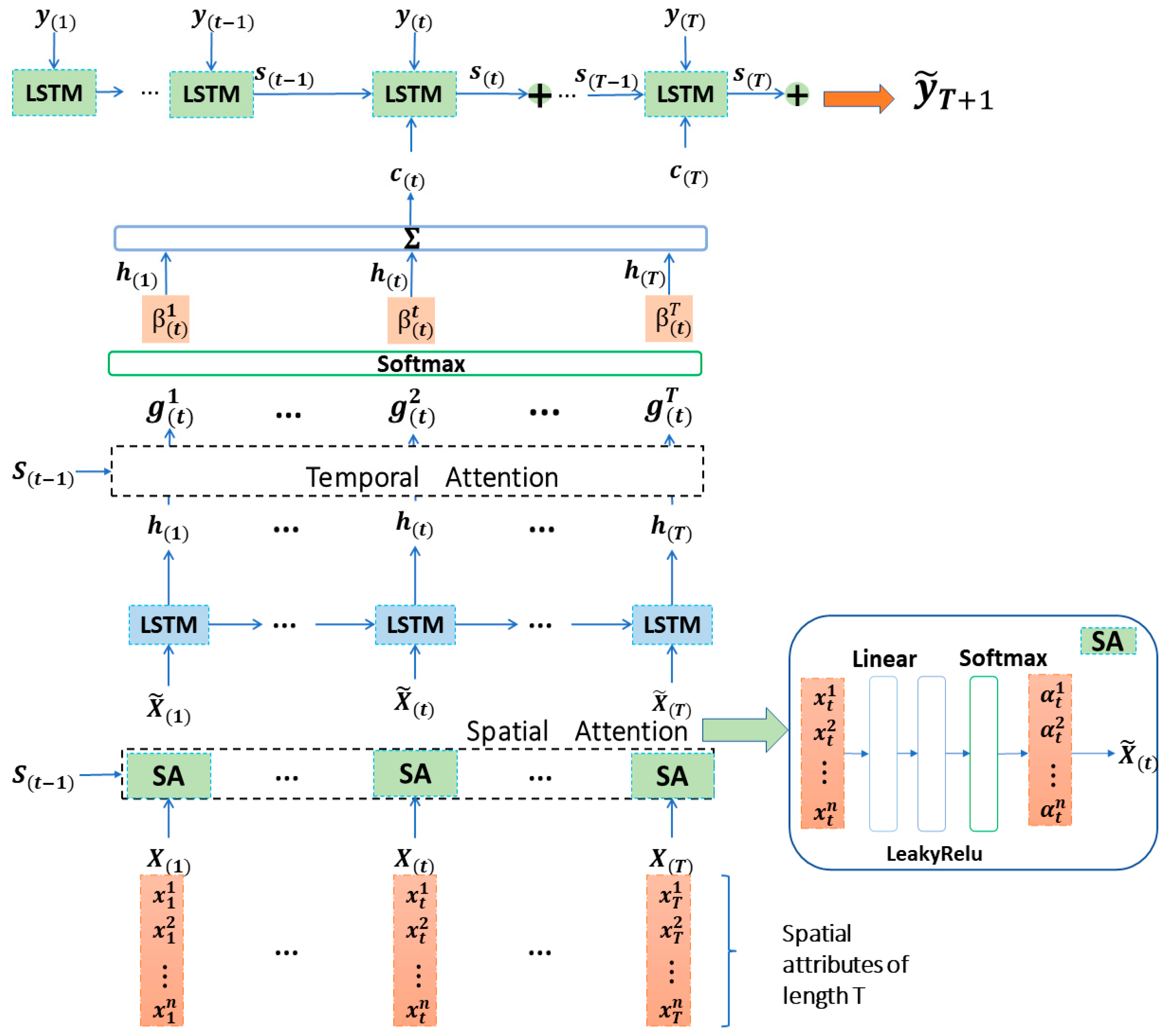
The overall structure of the STA-LSTM model is illustrated in Figure 2, which is based on an encoder–decoder network architecture with LSTM units as the backbone. The encoder includes a spatial attention mechanism module to adaptively identify important variables related to the target (i.e., water flow). Firstly, the spatial attention module calculates the weighted scores for different hydrological variables’ contributions to the target prediction, and the weighted variables are then input into the encoder LSTM network to update the hidden states. The decoder contains a temporal attention mechanism module to dynamically identify important hidden states related to the prediction variable. The hidden vectors at different time steps obtained from the encoder layer are input into the temporal attention mechanism module, which distinguishes crucial information in a weighted manner and forms a context vector for inputting into the decoder. Subsequently, the decoder LSTM network decodes the context vector and predicts the target flow data through a fully connected layer. Details of the STA-LSTM model will be elaborated on later in the paper.

3.2. LSTM

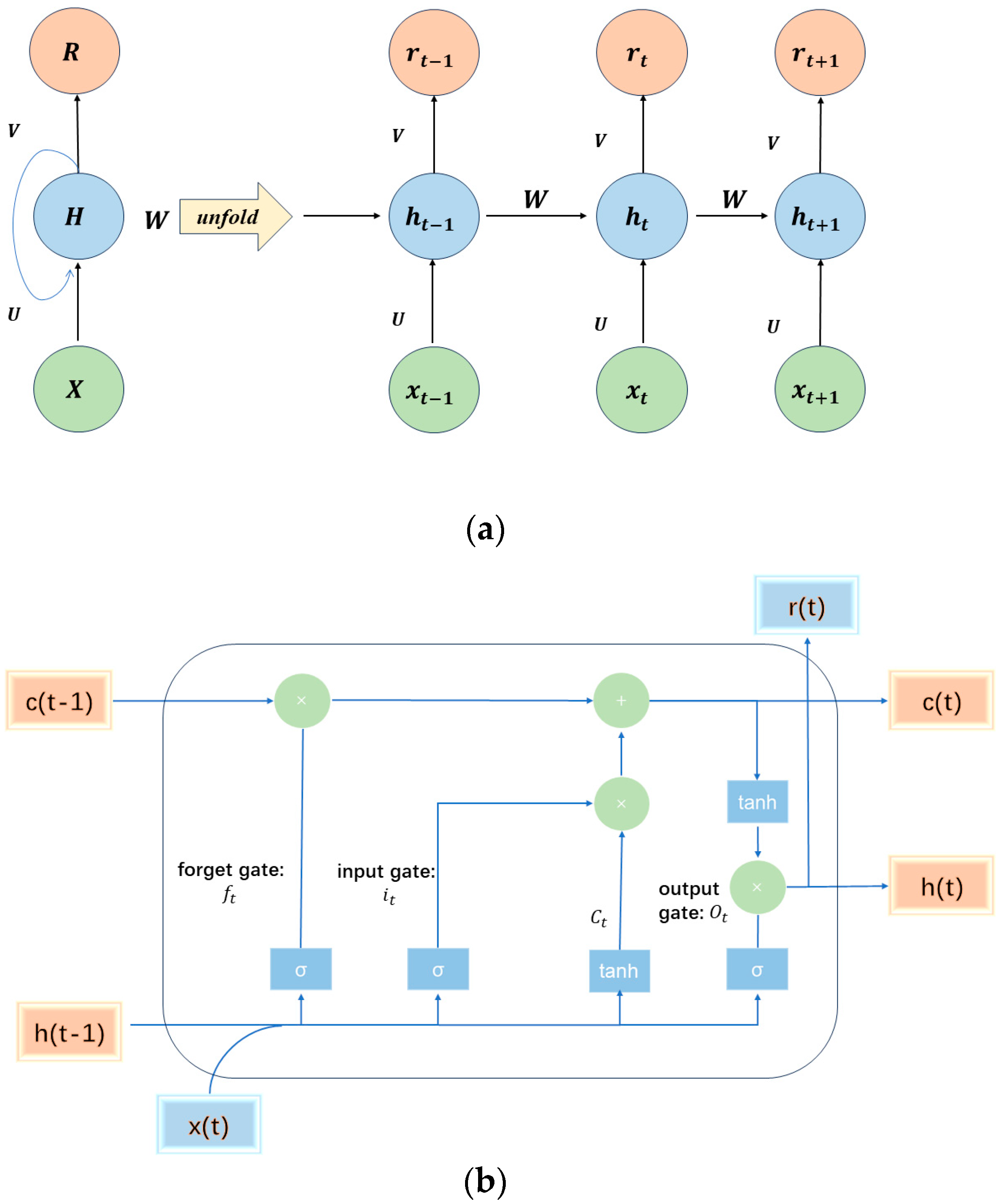
The Long Short-Term Memory (LSTM), proposed by Hochreiter and Schmidhuber [18] and further developed and popularized by Alex Graves [38], is now widely used in the field of machine learning. The basic structure of its recursive module is illustrated in Figure 3a. For intuitive representation, the output of the hidden module is set to be feedback to the input. Therefore, based on the current input x ( t ) and the previous hidden state h ( t 1 ) , the hidden state h ( t ) and the output r ( t ) at step t are obtained. The computation formula of the basic recursive unit is as follows:
r t = g V h t
h t = f U x t + W h t 1
The functions f and g are nonlinear activation functions. U , W , and V are the connection weights, which are shared across different time steps. The network specifies the hidden layer through the designed LSTM module, which performs well in handling the issues of gradient vanishing and exploding. The specific structure of each basic recursive unit in the LSTM network is shown in Figure 3b, which includes three inputs c ( t 1 ) , h ( t 1 ) , and x ( t ) , representing the unit state at the previous time step, the hidden state at the previous time step, and the current input, respectively. The LSTM contains three gate controllers: the forget gate, input gate, and output gate, used to determine what information should be forgotten, remembered, and outputted, respectively. Their computation formulas are as follows:
f t = σ W f x x t + W f h h t 1 + b f
i t = σ W i x x ~ t + W i h h t 1 + b i
o t = σ W o x x t + W o h h t 1 + b o
In the subsequent sections, the values computed from spatial and temporal attention serve as inputs to the encoder and decoder-side LSTMs to obtain the prediction results.

3.3. Encoder Decoder with Self-Attention

The encoder–decoder framework is a commonly used framework in deep learning to address sequence-to-sequence modeling problems [39]. By using RNN or other recursive neural networks, the encoder–decoder can effectively capture long-term dependencies in sequences, making it perform exceptionally well in many sequence modeling tasks such as language modeling and time series prediction. Compared to traditional RNN models, LSTM can effectively alleviate the accumulated prediction errors, showing significant advantages in handling data with long-term sequential features. Therefore, we utilize LSTM networks as the backbone network in the encoder–decoder layers of the flow prediction model.
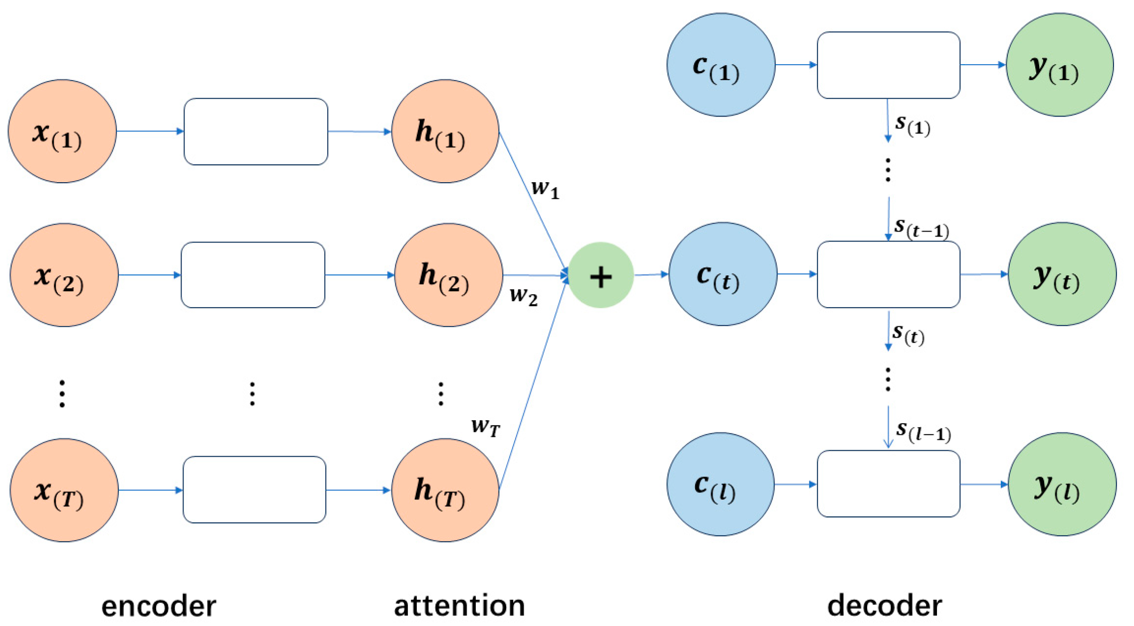
However, as the length of the input sequence increases, long-term information has less impact on the present, limiting the performance of predictions [40,41]. To address this issue, the attention mechanism is introduced into the encoder–decoder framework [42,43]. The structure of the attention-based encoder–decoder model is shown in Figure 4. Different vectors c ( t ) are designed instead of fixed ones for y ( t ) and can be calculated as
c t = i = 1 T w i h i
For the prediction at time step t, the attention mechanism assigns separate attention weights w ( i ) to each encoded hidden feature state h ( i ) based on its relationship with the previous hidden state in the decoder. In this study, the encoder transforms the input sequences, such as meteorological factors, into a sequence of hidden states, which is further transformed into a fixed-length vector and the decoder then utilizes it to predict the target output sequence. The encoder and decoder are trained end-to-end, typically executed in a sliding window manner, where the input and output sequences are progressively processed within a given window. Below, we specifically introduce the spatial attention and temporal attention mechanisms adopted in the encoder and decoder, respectively.

3.4. Spatial Attention with Encoder

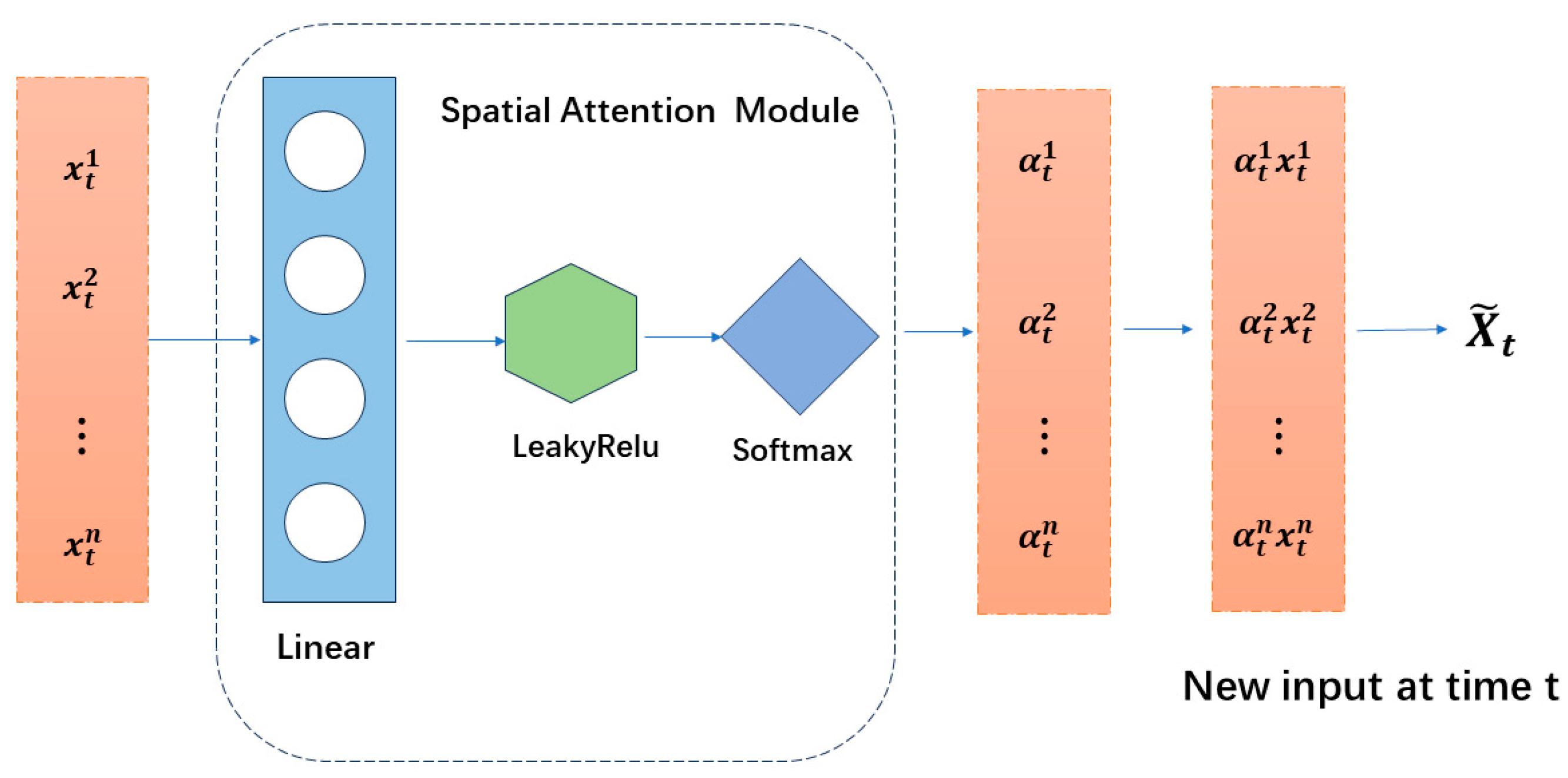
The encoder, serving as a feature extractor, represents the input data sequence as a fixed-length encoding vector, capturing the intrinsic correlations among the input auxiliary variable sequences. However, as the input sequence length increases, the encoder can only compute intermediate values to represent the original input sequence and struggles to individually capture the key features related to the prediction target from a large number of input sequences. Therefore, we introduce a spatial attention mechanism at the encoder layer to adaptively acquire the importance of pump station data and weather data for the flow prediction results relative to each geographical location, which is illustrated in Figure 5.
( x t 1 , x t 2 x t n ) represents the given feature at time step t and n is the number of auxiliary prediction variables. We capture the relationship between each input variable and the water flow by utilizing the previous decoder hidden state s t 1 , which is computed by measuring the similarity between the current raw input x ( t ) and the previous hidden state. Generally, a two-layer network structure is employed to extract the spatial attention between different variables. The spatial attention values e t i for each variable at each time step t are calculated as follows:
e t i = V 1 i L e a k y R e L u W 1 i s t 1 + U 1 i x t i + b 1 i     1 i n
where W 1 i , U 1 i , and b 1 i represent the fully connected layer weights and bias terms of a multi-layer perceptron, and LeakyReLU denotes a nonlinear activation function. e t i signifies the spatial attention for each variable, indicating the importance of the i-th input for flow prediction at time t. To ensure the sum of attention values for all input variables equals 1 at each sampling time t, the values of e t i are normalized as follows:
α t i = e t i j = 1 n e t j     1 i n
The normalized spatial attention weights α t i are utilized to adjust the importance of each feature vector, reflecting its relevance with the water flow prediction target. Therefore, the samples weighted by spatial attention can be represented as follows:
X ~ t = α t 1 x t 1 , α t 2 x t 2 , , α t n x t n
Then, we feed the attention-weighted input data into the encoder LSTM network to compute the context hidden states, which assist the model in memorizing crucial information to enhance prediction accuracy.

3.5. Temporal Attention with Decoder

Data are sequentially input into the encoder, where information carried by the previous timestep interacts with that of the subsequent timestep to contribute better prediction. However, due to interference from data noise, the accuracy of information carried by different timesteps is unbalanced. This situation may lead to relevant information being obscured by irrelevant data, and this issue becomes more severe with an increase in the length of the input time series. To alleviate this problem, we introduce a module of time attention mechanism at the decoder layer. This module dynamically identifies important hidden states similar to the prediction target across all timesteps, i.e., how the water plant flow at the prediction timestep depends on hydrological information at each timestep, which is shown in Figure 6.
In this study, the time feature represents hydrological data at different time points along the Eastern Route. After processing the input adjusted by spatial attention, the time attention module calculates the task-related weight for each timestep by analyzing the hidden states of the encoder. These weights indicate the importance of each timestep for the current prediction task. For each timestep within a sliding window before timestep t, the time attention of the hidden state is calculated as
g t k = V 2 k t a n h W 2 k s t 1 + U 2 k h t T + k + b 2 k     1 k T
where V 2 k , W 2 k , U 2 k , and b 2 k are learnable parameters related to the sample in the window, s t 1 is the previous timestep’s decoder hidden states, k is the sub-window size, and tanh is the hyperbolic tangent nonlinear activation function. The temporal attention is then normalized as follows:
β t k = g t k m = 1 T g t m     1 k T
This ensures that the sum of attention weights for all timesteps is equal to 1. The weighted context vector is calculated using the time attention weights, and this vector serves as the input to the decoder LSTM:
c t = k = 1 T h t T + k β t k
The time context vector c t varies at each timestep, and is then combined with one of the historical target data y t and input into the LSTM unit to update the decoder hidden state for the next timestep:
s t = f l y t , c t , s t 1
Here, the function f l represents the calculations of the LSTM unit, s t represents the updated decoder hidden state at timestep t and s t 1 is the previous decoder hidden state. This process iterates for each timestep of the sequence, allowing the model to capture the temporal dependencies for accurate prediction. By iteratively computing this process until s T 1 , the final LSTM unit in the decoder is able to generate the predicted target flow:
y ^ T + 1 = F ( y 1 , y 2 , , y T , x 1 , x 2 ,   , x T ) = V f l y T , c T , s T 1 + b v
F() is our deep learning network to predict the target, and the data of x and y in a sliding window of the previous 16 h are used to predict the data of the next half hour. We employ the Adam optimizer to train the model parameters, which offers superior computational time and less memory requirements compared to the traditional gradient descent with momentum. The model parameters are learned through standard backpropagation through time to minimize the Mean Squared Error (MSE) loss. The MSE measures the average of the squared errors, which is the average squared difference between the predicted values and the ground truth. The MSE is computed as follows:
M S E = 1 n i = 1 n y i ~ y i 2
where y i ~ denotes the predicted flow values, y i represents the ground truth flow values, and n is the number of test samples.

4. Results and Discussion

4.1. Evaluation Metrics

To evaluate the performance of the model, we use several performance metrics including Mean Absolute Error (MAE), Root Mean Square Error (RMSE), Mean Absolute Percentage Error (MAPE), and the coefficient of determination (R2). MAE is the average of the absolute differences between the predicted values and the actual values. The formula is as follows:
M A E = 1 n i = 1 n y i ~ y i
where y i ~ represents the predicted flow values, and y i represents the actual flow values. RMSE evaluates the accuracy of the regression results:
R M S E = 1 n i = 1 n y i ~ y i 2
MAPE is the Mean Absolute Percentage Error:
M A P E = 100 % n i = 1 n y i ~ y i y i
R 2 represents the correlation between two random variables and is calculated as
R 2 = 1 i = 1 n y i ~ y i 2 i = 1 n y i y i ̄ 2
where y i ̄ represents the mean of the true value sequence.

4.2. Hyperparameter Analysis

In this section, we analyze the model’s performance in relation to key hyperparameters, including the number of hidden neurons p and q in the encoder and decoder LSTM layers, and the window size T. We tune p and q using a grid search over {40, 60, 80, 100, 120}. Figure 7a illustrates RMSE for different hidden neuron numbers and window sizes. We select 40 hidden neurons to be optimal, which offer sufficient capacity without excessive complexity compared to 120.
The window size is searched in {8, 16, 32, 48, 96, 120}, as shown in Figure 7b. A higher or lower window size leads to a waste of performance and a decrease in accuracy. As sequence length increased, initial prediction errors decreased due to more historical data. However, longer sequences slow performance improvement as LSTM struggled with extensive historical dependencies. We choose a window size of 32 and obtain the best results. We also adjust other hyperparameters, such as neural network layers, to optimize performance and maintain robustness across conditions.
In studying the impact of the attention module on the STA-LSTM model, we specifically investigate the effects of different activation combinations. LeakyReLU is used in the spatial attention part for its ability to handle shallow features concentrated in a small range. Its advantage lies in maintaining gradients even for negative inputs, preventing neuron inactivity, and preserving feature distinctiveness for clearer weight distribution in subsequent Softmax operations. For the time attention part, we choose tanh due to its balanced treatment of positive and negative vector inputs, essential for timestep features. The results in Table 2 show that models using the LeakyReLU–tanh activation combination perform best and demonstrate stable performance. To ensure model robustness, we select the LeakyReLU–tanh combination as the final activation setting.

4.3. Experiment Settings

For all experimental data, 80% of the data are allocated for the training phase, with the remaining 20% used for testing. The model parameters are set with input feature dimensions fixed at 12, processing 128 samples per batch, a learning rate of 0.001, and a maximum training epoch of 200. We define a look-back window of 32 timesteps. We conduct all experiments with five different random seeds and average the results to obtain a fair comparison. At the end of each training epoch, we compute MAE, RMSE, MAPE, and R2 on the test set to monitor changes in model performance. All experiments are conducted on a computer equipped with an Intel(R) Xeon(R) CPU i5-13500H and NVIDIA GeForce RTX™ 3050 GPU.

4.4. Results and Analysis

4.4.1. Performance Comparison

We compare the proposed STA-LSTM model with the following baselines:
LSTM (Long Short-Term Memory network): a variant of Recurrent Neural Networks (RNNs) capable of learning long-term dependencies, commonly used in time series prediction.
GRU [44] (Gated Recurrent Unit): a variant of LSTM networks, it enhances computational efficiency by simplifying the temporal unit structure.
CNN (Convolutional Neural Network): a type of neural network with characteristics such as local connections and weight sharing, commonly used in deep feed-forward neural networks.
CNN-LSTM [45] (Combination of Convolutional Neural Network (CNN) and LSTM): a combination where CNN is used to extract spatial features from time series data and LSTM is used for temporal sequence processing.
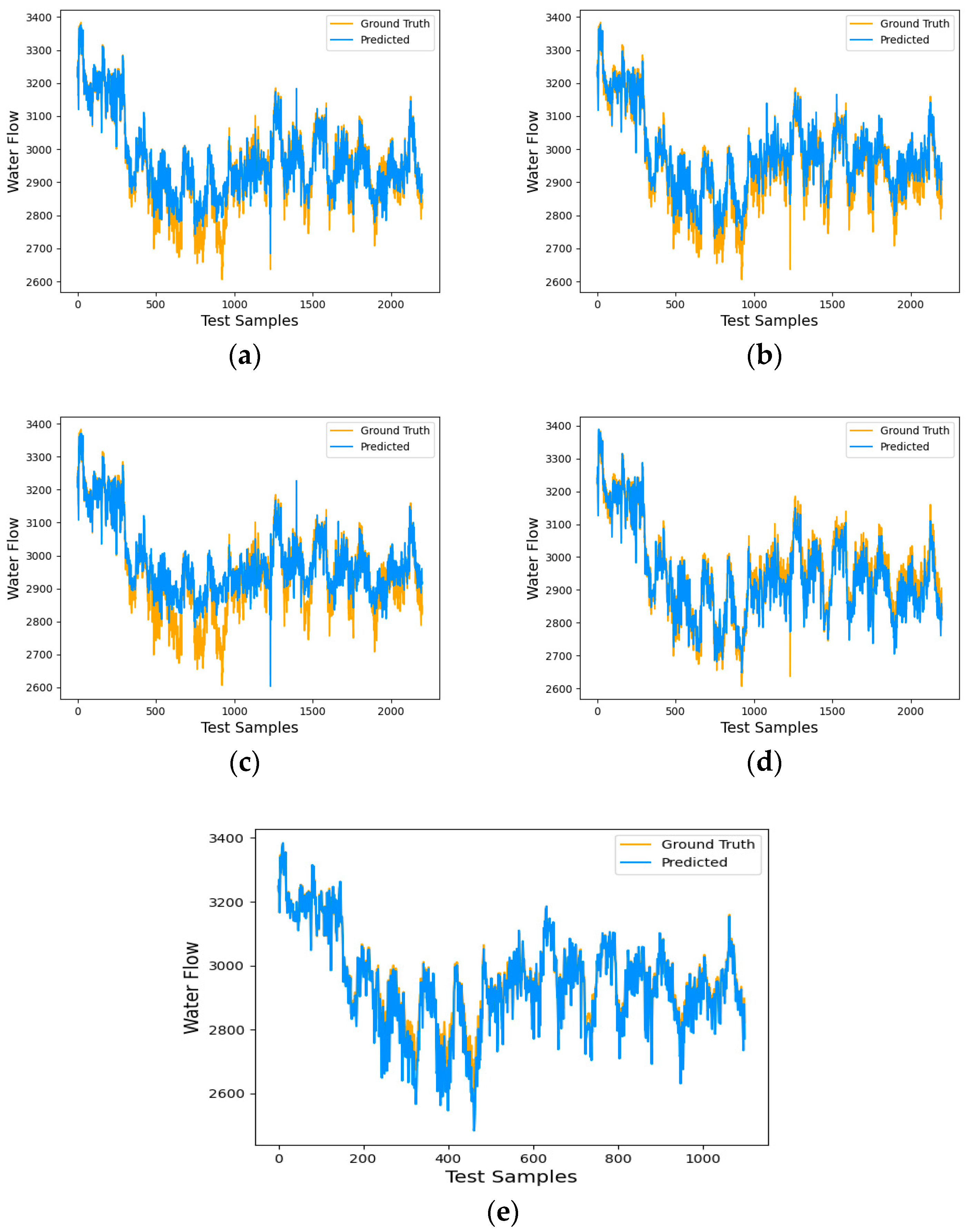
The experimental parameter settings are shown in Table 3. A detailed prediction of water plant flow is shown in Figure 8, and experimental performance results are shown in Table 4.
Quantitative experiments demonstrate that the STA-LSTM model outperforms other models significantly in key metrics such as MAE, RMSE, and MAPE. Additionally, the R2 value approaching 1 indicates its outstanding accuracy and generalization ability. Furthermore, the predictions of each model on the test set are shown in Figure 8. As indicated in Table 4, the STA-LSTM model exhibits the lowest MAE and RMSE, corresponding to prediction curves that closely align with the truth water flow curve, demonstrating higher accuracy compared to all baselines.

4.4.2. Ablation Study

In this section, we examine the influence of meteorological condition variables on prediction accuracy. The results presented in Table 5 reveal that models incorporating meteorological data achieve higher prediction accuracy. This observation is consistent with real-world dynamics, where increased rainfall correlates with greater upstream water volume, thereby impacting the flow along the pipeline.
Subsequently, we conduct a systematic analysis by sequentially removing the Spatial Attention (SA) and Temporal Attention (TA) modules from the STA-LSTM model to assess their respective contributions. SA-LSTM integrates a spatial attention mechanism within the encoder to emphasize critical spatial features in the input data. In contrast, TA-LSTM incorporates a temporal attention mechanism within the decoder to assign varying levels of significance to different time steps.
The results, as presented in Table 6, indicate a significant decrease in prediction accuracy when either module is removed. SA-LSTM could not effectively address the issue of memory decay that can occur in long sequences, leading to increased prediction errors. Conversely, TA-LSTM may suffer from limitations in handling multivariate spatial features due to the lack of spatial attention mechanisms.

4.4.3. Visual Attention Analysis

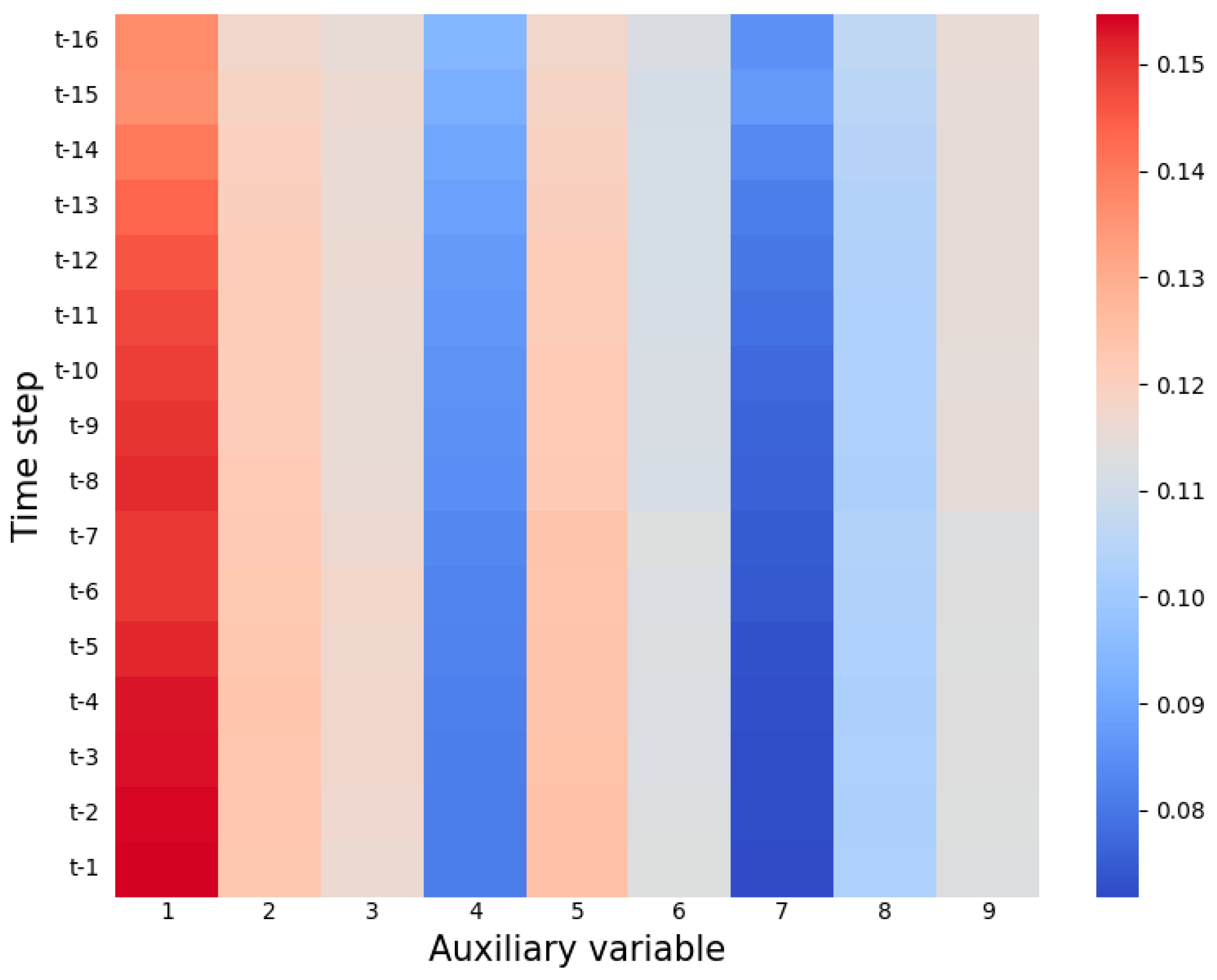
In this section, we visualize the attention weights of the proposed STA-LSTM model and analyze the trend. To better analyze the correlation between pumping station data and water plant flows, a hydrologic dataset without weather is used here. It contains 9-dimensional pumping station data and the variables are in the same order as the full dataset. The attention weight distribution on the hydrological dataset is shown in Figure 9 when predicting the water flow at the current time step t of the water plant. We observe that the first and fifth spatial attributes (i.e., the pressure at point A pump station and the water level in front of point B pump station), as well as the second spatial attribute (i.e., the water level in front of point A pump station), exhibit darker colors than other spatial attributes across most historical timesteps. This implies their higher importance throughout the entire prediction process and thus, they are assigned greater weights.

4.5. Discussion

Among the experimental results mentioned above, STA-LSTM demonstrates higher accuracy compared to other methods. These findings are supported by the data presented in Table 4, where STA-LSTM consistently achieves significantly lower values across all error metrics. This indicates its superiority in capturing complex spatiotemporal relationships and delivering precise predictions. The average absolute error (MAE) for STA-LSTM is 3.57, the root mean square error (RMSE) is 4.61, and the mean absolute percentage error (MAPE) is 0.001, demonstrating enhanced predictive performance. We find that the performance differences among the models mainly stem from their ability to handle spatiotemporal relationships and sequential data. While both GRU and LSTM can maintain long-term dependencies in time series, the simplicity of GRU’s structure may lead to the loss of important information, resulting in a lower performance compared to LSTM. However, neither of these models effectively captures spatial and temporal information, leading to poor predictive performance. SLSTM, due to its simplistic feature extraction and lack of attention mechanisms, shows an inferior performance. Although CNN-LSTM extracts spatial information, it still has limitations in handling complex spatiotemporal data, hence its subpar performance.
Ablation study suggests that both SA and TA modules play vital roles in capturing spatiotemporal dependencies. STA-LSTM proves the crucial significance of its strategy in comprehensively leveraging spatiotemporal information for performance enhancement. The results of the visual experiment analysis are consistent with the logic of the hydrological system. When the opening of Shijingshan gate is certain, point A (Yuquanshan pump Station) is located in the upstream area, and its pipeline pressure directly affects the flow of the downstream Shijingshan gate. The variation of water level in the lower reaches of Xingshikou implies the inherent constraint of the data of hydrographic stations in the upper and lower reaches, which plays a key role in predicting the water quantity of Shijingshan.
Our STA-LSTM model, with its unique spatiotemporal attention mechanism, effectively utilizes both spatial and temporal information, enhancing its ability to capture complex spatiotemporal patterns and demonstrating exceptional performance in the task of predicting water flow.

5. Conclusions

To address the strong nonlinearity and dynamics of hydrological problems in flow prediction tasks, we propose the improved STA-LSTM model. Building upon the LSTM backbone network, our model incorporates a spatial attention mechanism in the encoding layer and introduces a time attention mechanism in the decoding layer. This allows the model to adaptively determine the information relevant to the predicted flow from the input hydrological data, and dynamically distinguish important hidden states related to flow velocity from the output of the encoder.
To validate the effectiveness of the proposed STA-LSTM, we construct a real dataset containing data from three adjacent pumping stations and external meteorological data. Extensive experiments show that the STA-LSTM model outperforms all baselines. Specifically, it achieved reductions of 20.16 in MAE, 24.84 in RMSE, and 0.007 in MAPE, and a 3.96% increase in R2 compared to the baseline model. STA-LSTM provides valuable insights for the future application and promotion of deep learning methods in fields such as water supply system management.
The STA-LSTM model proposed in this study demonstrates efficient training and accurate prediction on conventional computing platforms. However, in the context of automated pumping stations, the issue of delayed prediction result generation remains to be addressed. Future research will focus on developing a lightweight multi-step flow prediction model to tackle these challenges.

Author Contributions

Conceptualization, W.H.; data curation, W.H. and X.S.; methodology, W.H. and J.Y.; software, W.H.; supervision, J.Y., W.H., Y.Y., Z.Z., W.S. and X.S.; validation, W.H. and Y.Y.; writing—original draft, W.H. All authors have read and agreed to the published version of the manuscript.

Funding

This research received no external funding.

Data Availability Statement

The data in this study can be obtained by contacting the author’s email.

Acknowledgments

The authors would like to thank the anonymous reviewers for their valuable comments and suggestions, which helped improve this paper greatly.

Conflicts of Interest

The authors declare no conflicts of interest.

References

  1. Nguyen, T.T.; Ngo, H.H.; Guo, W.; Wang, X.C.; Ren, N.; Li, G.; Ding, J.; Liang, H. Implementation of a specific urban water management-Sponge City. Sci. Total Environ. 2019, 652, 147–162. [Google Scholar] [CrossRef] [PubMed]
  2. Jain, S.K.; Singh, V.P. Water Resources Systems Planning and Management; Elsevier: Amsterdam, The Netherlands, 2023; ISBN 0323984126. [Google Scholar]
  3. Ghorani, M.M.; Haghighi, M.H.S.; Maleki, A.; Riasi, A. A numerical study on mechanisms of energy dissipation in a pump as turbine (PAT) using entropy generation theory. Renew. Energy 2020, 162, 1036–1053. [Google Scholar] [CrossRef]
  4. Yan, P.; Zhang, Z.; Lei, X.; Hou, Q.; Wang, H. A multi-objective optimal control model of cascade pumping stations considering both cost and safety. J. Clean. Prod. 2022, 345, 131171. [Google Scholar] [CrossRef]
  5. Lu, L.; Tian, Y.; Lei, X.; Wang, H.; Qin, T.; Zhang, Z. Numerical analysis of the hydraulic transient process of the water delivery system of cascade pump stations. Water Sci. Technol. Water Supply 2018, 18, 1635–1649. [Google Scholar] [CrossRef]
  6. Shi, L.; Zhang, W.; Jiao, H.; Tang, F.; Wang, L.; Sun, D.; Shi, W. Numerical simulation and experimental study on the comparison of the hydraulic characteristics of an axial-flow pump and a full tubular pump. Renew. Energy 2020, 153, 1455–1464. [Google Scholar] [CrossRef]
  7. Rashidov, J.; Kholbutaev, B. Water distribution on machine canals trace cascade of pumping stations. In IOP Conference Series: Materials Science and Engineering; IOP Publishing: Bristol, UK, 2020; p. 12066. [Google Scholar]
  8. Assem, H.; Ghariba, S.; Makrai, G.; Johnston, P.; Gill, L.; Pilla, F. Urban water flow and water level prediction based on deep learning. In Proceedings of the Machine Learning and Knowledge Discovery in Databases: European Conference, ECML PKDD 2017, Skopje, Macedonia, 18–22 September 2017; Proceedings, Part III 10. pp. 317–329. [Google Scholar]
  9. Cisty, M.; Soldanova, V. Flow prediction versus flow simulation using machine learning algorithms. In Machine Learning and Data Mining in Pattern Recognition. In Proceedings of the 14th International Conference, MLDM 2018, New York, NY, USA, 15–19 July 2018; Proceedings, Part II 14. pp. 369–382. [Google Scholar]
  10. Yuan, X.; Chen, C.; Lei, X.; Yuan, Y.; Muhammad Adnan, R. Monthly runoff forecasting based on LSTM–ALO model. Stoch. Environ. Res. Risk Assess. 2018, 32, 2199–2212. [Google Scholar] [CrossRef]
  11. Ahmed, A.N.; Othman, F.B.; Afan, H.A.; Ibrahim, R.K.; Fai, C.M.; Hossain, M.S.; Ehteram, M.; Elshafie, A. Machine learning methods for better water quality prediction. J. Hydrol. 2019, 578, 124084. [Google Scholar] [CrossRef]
  12. Li, X.; Xu, W.; Ren, M.; Jiang, Y.; Fu, G. Hybrid CNN-LSTM models for river flow prediction. Water Supply 2022, 22, 4902–4919. [Google Scholar] [CrossRef]
  13. Fathian, F.; Mehdizadeh, S.; Kozekalani Sales, A.; Safari, M.J.S. Hybrid models to improve the monthly river flow prediction: Integrating artificial intelligence and non-linear time series models. J. Hydrol. 2019, 575, 1200–1213. [Google Scholar] [CrossRef]
  14. Khazaee Poul, A.; Shourian, M.; Ebrahimi, H. A Comparative Study of MLR, KNN, ANN and ANFIS Models with Wavelet Transform in Monthly Stream Flow Prediction. Water Resour. Manag. 2019, 33, 2907–2923. [Google Scholar] [CrossRef]
  15. Zhang, J.; Zhu, Y.; Zhang, X.; Ye, M.; Yang, J. Developing a Long Short-Term Memory (LSTM) based model for predicting water table depth in agricultural areas. J. Hydrol. 2018, 561, 918–929. [Google Scholar] [CrossRef]
  16. Zaremba, W.; Sutskever, I.; Vinyals, O. Recurrent neural network regularization. arXiv 2014, arXiv:1409.2329. [Google Scholar]
  17. Zhou, Y.; Guo, S.; Xu, C.; Chang, F.; Yin, J. Improving the reliability of probabilistic multi-step-ahead flood forecasting by fusing unscented Kalman filter with recurrent neural network. Water 2020, 12, 578. [Google Scholar] [CrossRef]
  18. Hochreiter, S.; Schmidhuber, J. Long short-term memory. Neural Comput. 1997, 9, 1735–1780. [Google Scholar] [CrossRef]
  19. Le, X.; Ho, H.V.; Lee, G.; Jung, S. Application of long short-term memory (LSTM) neural network for flood forecasting. Water 2019, 11, 1387. [Google Scholar] [CrossRef]
  20. Hu, Y.; Yan, L.; Hang, T.; Feng, J. Stream-Flow Forecasting of Small Rivers Based on LSTM. arXiv 2020, arXiv:2001.05681. [Google Scholar]
  21. Bahdanau, D.; Cho, K.; Bengio, Y. Neural Machine Translation by Jointly Learning to Align and Translate. arXiv 2014, arXiv:1409.0473. [Google Scholar]
  22. Kroner, A.; Senden, M.; Driessens, K.; Goebel, R. Contextual encoder–decoder network for visual saliency prediction. Neural Netw. 2020, 129, 261–270. [Google Scholar] [CrossRef]
  23. Zhu, S.; Luo, X.; Yuan, X.; Xu, Z. An improved long short-term memory network for streamflow forecasting in the upper Yangtze River. Stoch. Environ. Res. Risk Assess. 2020, 34, 1313–1329. [Google Scholar] [CrossRef]
  24. Zounemat-Kermani, M.; Mahdavi-Meymand, A.; Hinkelmann, R. A comprehensive survey on conventional and modern neural networks: Application to river flow forecasting. Earth Sci. Inform. 2021, 14, 893–911. [Google Scholar] [CrossRef]
  25. Alizadeh, B.; Ghaderi Bafti, A.; Kamangir, H.; Zhang, Y.; Wright, D.B.; Franz, K.J. A novel attention-based LSTM cell post-processor coupled with bayesian optimization for streamflow prediction. J. Hydrol. 2021, 601, 126526. [Google Scholar] [CrossRef]
  26. Xie, Z.; Du, Q.; Ren, F.; Zhang, X.; Jamiesone, S. Improving the forecast precision of river stage spatial and temporal distribution using drain pipeline knowledge coupled with BP artificial neural networks: A case study of Panlong River, Kunming, China. Nat. Hazards 2015, 77, 1081–1102. [Google Scholar] [CrossRef]
  27. Fu, Y.; Wang, X.; Wei, Y.; Huang, T. STA: Spatial-Temporal Attention for Large-Scale Video-based Person Re-Identification. In Proceedings of the AAAI Conference on Artificial Intelligence, Honolulu, HI, USA, 27 January 2019–1 February 2019. [Google Scholar]
  28. Chang, L.; Liou, J.; Chang, F. Spatial-temporal Flood Inundation Nowcasts by Fusing Machine Learning Methods and Principal Component Analysis. J. Hydrol. 2022, 612, 128086. [Google Scholar] [CrossRef]
  29. Noor, F.; Haq, S.; Rakib, M.; Ahmed, T.; Jamal, Z.; Siam, Z.S.; Hasan, R.T.; Adnan, M.S.G.; Dewan, A.; Rahman, R.M. Water Level Forecasting Using Spatiotemporal Attention-Based Long Short-Term Memory Network. Water 2022, 14, 612. [Google Scholar] [CrossRef]
  30. Wang, Y.; Huang, Y.; Xiao, M.; Zhou, S.; Xiong, B.; Jin, Z. Medium-long-term prediction of water level based on an improved spatio-temporal attention mechanism for long short-term memory networks. J. Hydrol. 2023, 618, 129163. [Google Scholar] [CrossRef]
  31. Li, H.; Cao, P.; Wang, X.; Yi, B.; Huang, M.; Sun, Q.; Zhang, Y. Multi-task spatio-temporal augmented net for industry equipment remaining useful life prediction. Adv. Eng. Inform. 2023, 55, 101898. [Google Scholar] [CrossRef]
  32. Chen, C.; Zhou, H.; Zhang, H.; Chen, L.; Yan, Z.; Liang, H. A Novel Deep Learning Algorithm for Groundwater Level Prediction Based on Spatiotemporal Attention Mechanism; Creative Commons: Mountain View, CA, USA, 2020. [Google Scholar]
  33. Lin, T.; Pan, Y.; Xue, G.; Song, J.; Qi, C. A Novel Hybrid Spatial-Temporal Attention-LSTM Model for Heat Load Prediction. IEEE Access 2020, 8, 159182–159195. [Google Scholar] [CrossRef]
  34. Linardatos, P.; Papastefanopoulos, V.; Kotsiantis, S. Explainable ai: A review of machine learning interpretability methods. Entropy 2020, 23, 18. [Google Scholar] [CrossRef]
  35. Li, X.; Xiong, H.; Li, X.; Wu, X.; Zhang, X.; Liu, J.; Bian, J.; Dou, D. Interpretable deep learning: Interpretation, interpretability, trustworthiness, and beyond. Knowl. Inf. Syst. 2022, 64, 3197–3234. [Google Scholar] [CrossRef]
  36. Ding, Y.; Zhu, Y.; Feng, J.; Zhang, P.; Cheng, Z. Interpretable spatio-temporal attention LSTM model for flood forecasting. Neurocomputing 2020, 403, 348–359. [Google Scholar] [CrossRef]
  37. Ghobadi, F.; Kang, D. Improving long-term streamflow prediction in a poorly gauged basin using geo-spatiotemporal mesoscale data and attention-based deep learning: A comparative study. J. Hydrol. 2022, 615, 128608. [Google Scholar] [CrossRef]
  38. Graves, A. Generating Sequences with Recurrent Neural Networks. arXiv 2014, arXiv:1308.0850. [Google Scholar]
  39. Sutskever, I.; Vinyals, O.; Le, Q.V. Sequence to sequence learning with neural networks. arXiv 2014, arXiv:1409.3215. [Google Scholar]
  40. Cho, K.; van Merriënboer, B.; Bahdanau, D.; Bengio, Y. On the Properties of Neural Machine Translation: Encoder–Decoder Approaches; Association for Computational Linguistics: Doha, Qatar, 2014; pp. 103–111. [Google Scholar] [CrossRef]
  41. Hassanin, M.; Anwar, S.; Radwan, I.; Khan, F.S.; Mian, A. Visual attention methods in deep learning: An in-depth survey. Inf. Fusion. 2024, 108, 102417. [Google Scholar] [CrossRef]
  42. Vaswani, A.; Shazeer, N.M.; Parmar, N.; Uszkoreit, J.; Jones, L.; Gomez, A.N.; Kaiser, L.; Polosukhin, I. Attention is All you Need. arXiv 2017, arXiv:1706.03762. [Google Scholar]
  43. Zheng, C.; Fan, X.; Wang, C.; Qi, J. Gman: A graph multi-attention network for traffic prediction. In Proceedings of the AAAI Conference on Artificial Intelligence, New York, NY, USA, 7–12 February 2020; pp. 1234–1241. [Google Scholar]
  44. Chung, J.; Gulcehre, C.; Cho, K.; Bengio, Y. Empirical evaluation of gated recurrent neural networks on sequence modeling. arXiv 2014, arXiv:1412.3555. [Google Scholar]
  45. Shi, X.; Chen, Z.; Wang, H.; Yeung, D.; Wong, W.; Woo, W. Convolutional LSTM network: A machine learning approach for precipitation nowcasting. arXiv 2015, arXiv:1506.04214. [Google Scholar]
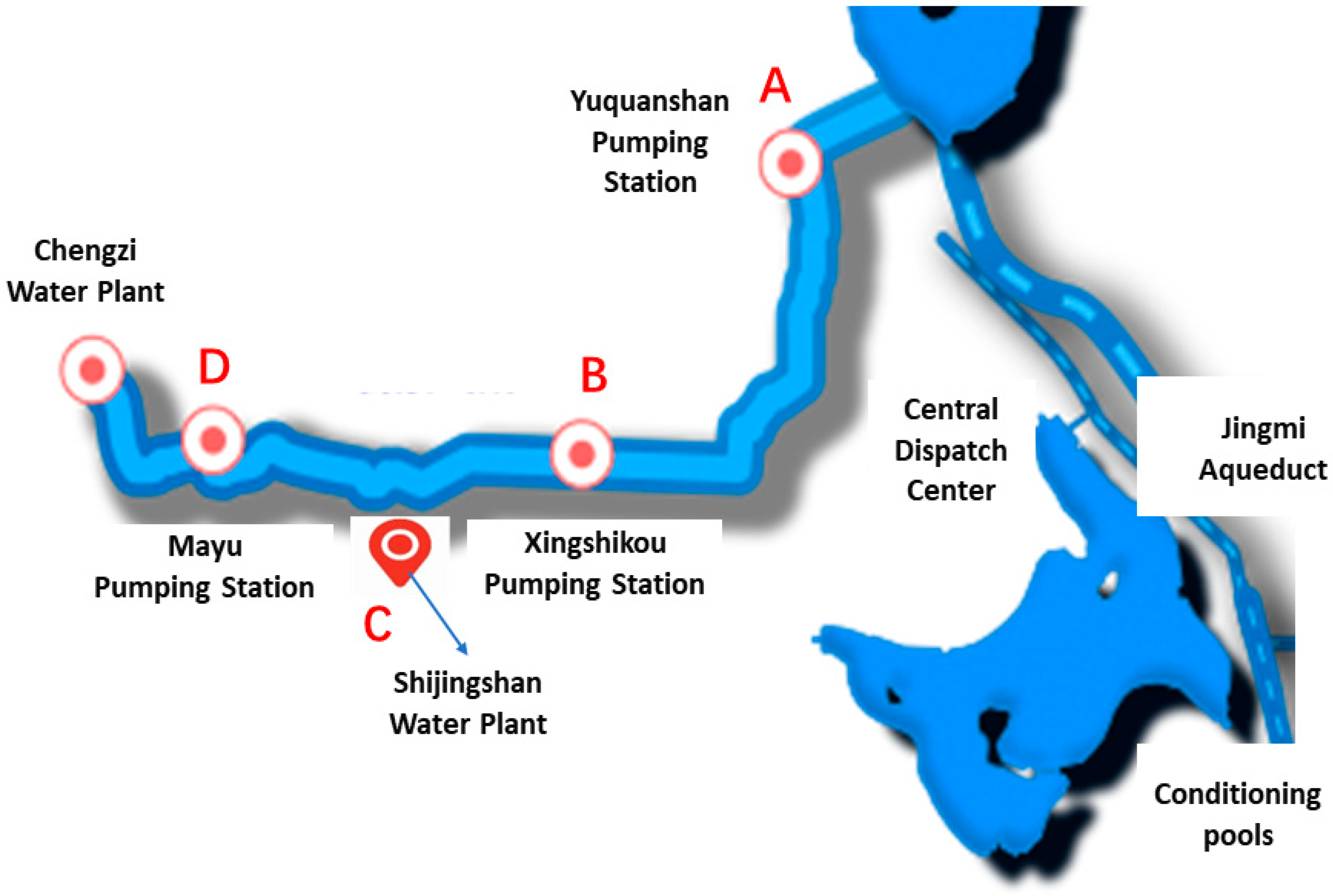
Figure 1. Schematic diagram of the distribution of water flow monitoring pump stations. Point A represents the upstream Yuquanshan pump station, point B represents the upstream Xingshikou pump station, point C represents the Shijingshan Water Plant, and point D represents the Mayu Pump Station. The line connecting the pumping station and the water plant on the left is the canal, the dashed blue line on the right is the Jingmi Diversion Canal, and the blue block is the regulating pool.
Water 16 01600 g001
Figure 2. Overall Framework of the STA-LSTM Model. X ( t ) = ( x t 1 , x t 2 x t n ) represents all input variables at time t. At each time step, the variables undergo spatial attention (SA) calculation simultaneously, and the weighted output   X ~ ( t ) is then produced with weights α . Following this, the hidden states within the window size T before time t undergo temporal attention (TA) calculation. The context c ( t )   after weighting the hidden state variable (weight g normalized to β) is input into the decoder, and the calculation is cycled to the end of the window c ( T ) input decoding unit output y ~ T + 1 .
Water 16 01600 g002
Figure 3. Sketch graphs of the basic recurrent module and the backbone LSTM unit. The introduction of hidden state allows the two modules to recurrently learn a sequence for the dynamic feature extraction. (a) Structure of a basic recurrent module; (b) structure of an LSTM module.
Water 16 01600 g003
Figure 4. Attention-based Encoder–Decoder Model Architecture.
Water 16 01600 g004
Figure 5. Encoder Layer with Spatial Attention Mechanism.
Water 16 01600 g005
Figure 6. Decoder Layer with Temporal Attention Mechanism.
Water 16 01600 g006
Figure 7. Effects of Hyperparameters on STA Model. (a) Number of Hidden Neurons Impact on MAE; (b) Window Size Impact on MAE.
Water 16 01600 g007
Figure 8. Detailed prediction results of water plant flow: (a) LSTM; (b) GRU; (c) CNN; (d) CNN-LSTM; (e) STA-LSTM.
Water 16 01600 g008
Figure 9. Visualization of Model Attention Map.
Water 16 01600 g009
Table 1. Units of input attributes.
Input AttributeDescriptionUnit
PIPE_PRESS (P)Pipeline pressureMpa
Water Level (H)Water level heightm
Water Flow (Q)Water flow ratem3/h
Rainfall (R)Local rainfallmm
Temperature (T)Local temperatures°C
Table 2. Comparison of model performance using different activation function combinations in STA-LSTM attention mechanisms.
Activation CombinationMAERMSER2
tanh–LeakyReLU3.955.740.974
tanh–ReLU3.935.700.976
ReLU–LeakyReLU3.955.740.974
LeakyReLU–tanh3.314.370.991
Table 3. Parameter settings of baseline models and our STA-LSTM model.
ModelsParameters
Learning RateRun UnitsActivation
LSTM0.001128tanh
GRU0.001128tanh
CNN0.001128tanh
CNN-LSTM0.001128ReLU
STA-LSTM0.001p = 60 *
q = 60 *
LeakyReLU–tanh
Note: * p and q are the number of hidden neurons in the encoder and decoder LSTM layers, respectively.
Table 4. Comparison of MAE, RMSE, MAPE, and R2 for the test set of each model in the test process.
ModelsMAERMSEMAPER2
LSTM26.7235.970.0090.9298
GRU29.0736.730.0100.9148
CNN41.7553.540.0150.8142
CNN-LSTM23.7329.450.0080.9516
STA-LSTM3.574.610.0010.9912
Table 5. Comparison of Evaluation Metrics for Test Sets of Different Models on Hydrological and Hydro-meteorological Datasets.
DatasetMAERMSEMAPER2
Hydrological data5.257.320.00230.9668
Hydrological and meteorological data3.574.610.00120.9912
Table 6. Comparison of Evaluation Metrics for Test Sets Under Different Attention Mechanisms.
ModelMAERMSEMAPER2
TA-LSTM23.4332.010.00810.9428
SA-LSTM19.5628.810.00690.9507
STA-LSTM3.574.610.00120.9912
Disclaimer/Publisher’s Note: The statements, opinions and data contained in all publications are solely those of the individual author(s) and contributor(s) and not of MDPI and/or the editor(s). MDPI and/or the editor(s) disclaim responsibility for any injury to people or property resulting from any ideas, methods, instructions or products referred to in the content.