Article

Runoff Prediction in Different Forecast Periods via a Hybrid Machine Learning Model for Ganjiang River Basin, China

1
National Institute of Natural Hazards, Ministry of Emergency Management of China, Beijing 100085, China
2
General Institute of Water Resources and Hydropower Planning and Design, Ministry of Water Resources, Beijing 100120, China
3
Hydrology and Water Resources Monitoring Center of Lower Ganjiang River, Yichun 336000, China
4
Nanjing Hydraulic Research Institute, Nanjing 210029, China
*
Author to whom correspondence should be addressed.
Water 2024, 16(11), 1589; https://doi.org/10.3390/w16111589
Submission received: 7 April 2024 / Revised: 25 May 2024 / Accepted: 30 May 2024 / Published: 1 June 2024

Abstract

:
Accurate forecasting of monthly runoff is essential for efficient management, allocation, and utilization of water resources. To improve the prediction accuracy of monthly runoff, the long and short memory neural networks (LSTM) coupled with variational mode decomposition (VMD) and principal component analysis (PCA), namely VMD-PCA-LSTM, was developed and applied at the Waizhou station in the Ganjiang River Basin. The process begins with identifying the main forecasting factors from 130 atmospheric circulation indexes using the PCA method and extracting the stationary components from the original monthly runoff series using the VMD method. Then, the correlation coefficient method is used to determine the lag of the above factors. Lastly, the monthly runoff is simulated by combining the stationary components and key forecasting factors via the LSTM model. Results show that the VMD-PCA-LSTM model effectively addresses the issue of low prediction accuracy at high flows caused by a limited number of samples. Compared to the single LSTM and VMD-LSTM models, this comprehensive approach significantly enhances the model’s predictive accuracy, particularly during the flood season.

1. Introduction

Runoff prediction is essential for water resource management, allocation, and effective utilization [1,2]. Accurate runoff prediction, especially in medium- and long-term timescales, can provide effective scientific support for agricultural irrigation, industrial and domestic water use, reservoir optimization, water conservancy project planning and design, etc. [3,4]. Another significant aspect of runoff prediction is providing early warnings for floods and drought, which are strongly correlated with certain meteorological factors, such as precipitation and runoff, as indicated by relevant studies [5,6]. However, due to its vulnerability to climate change and human activities, runoff has the characteristics of being highly nonlinear, unstable and complicated [7]. Therefore, it is still a challenge to obtain high-precision runoff-prediction results.
Currently, runoff prediction models can be divided into two types: process-driven models [8,9,10] and data-driven models [11,12,13]. Process-driven models are modeled to simulate complex non-linear physical hydrological process through a series of mathematical equations based on an understanding and simplification of the principles of the natural water system [14,15]. For example, the Xin’anjiang model [16], the Soil and Water Assessment Tool [17], and Sacramento Soil Moisture Accounting [18] are the most widely used physically driven models. Although they can reveal the physical mechanism of runoff generation [19,20], there is still another important factor that can affect the hydrological processes, e.g., human activities such as hydropower, which are processes hardly modeled using traditional physically based models. Additionally, the modeling demands a great deal of accurate and reliable information on hydrological processes (e.g., precipitation and evapotranspiration), which leads to common shortcomings such as difficulty in determining the parameters and poor versatility of the model. With improvements in computing power, data-driven models have shown great potential in capturing the rainfall–runoff relationship and predicting the runoff in a given basin. Without considering the hydrological physical processes, data-driven models are widely employed to address a variety of classification and regression problems by establishing the statistical relationships between inputs and outputs. For the prediction of medium- and long-term runoff, researchers have used data-driven models such as artificial neural networks (ANNs), support vector machines (SVMs), and long short-term memory (LSTM) networks to capture the nonlinear and unsteady characteristics of runoff time series [21,22,23], and some studies have achieved better performance than those using traditional process-driven models [24,25]. As a branch of data-driven models, deep learning models can better address the insufficient ability of classical data-driven models to deal with nonlinear relationships in difficult situations. Recently, with the rapid development of deep learning models, it has been increasingly studied in the simulation and prediction of hydrological elements such as runoff, evapotranspiration, and soil moisture [26,27,28]. For instance, Castangia et al. [29] explored the applicability of the transformer model to flood forecasting and found that the model has higher prediction accuracy than recurrent neural networks. Although many new deep learning models have been applied to the hydrologic forecasting field, long short-term memory (LSTM) still keeps a wide application in runoff prediction [30], especially for monthly runoff prediction.
In addition to the selection of appropriate hydrological models, identifying the key forecasting factors that drive runoff variability is another aspect of building a reliable forecast model [31]. Since runoff is a non-stationary component with periodicity, stochasticity, and trend, the accuracy of direct prediction using the above models is limited [32]. The signal decomposition technique can decompose the runoff series into several relatively stable components to reduce the non-stationarity of the time series with high complexity and strong nonlinear, which can help the model better capture the change patterns of the runoff series and improve the prediction accuracy [33,34]. For example, Wang et al. [35] found that the runoff prediction results of the auto-regressive integrated moving average (ARIMA) model combined with the ensemble empirical mode decomposition (EEMD) are more accurate and stable than that of a single ARIMA model. Zuo et al. [36] developed a single-model forecasting (SF) scheme based on variational mode decomposition (VMD) and LSTM to predict daily runoff with a lead time of 1–7 days, and found that the SF-VMD-LSTM can effectively capture the unsteady and nonlinear nature of the runoff. Additionally, previous studies have shown that the rainfall–runoff process is also closely connected with climatic conditions and human activities except for traditional meteorological factors such as precipitation and potential evapotranspiration [37,38]. Champagne et al. [39] quantified the contribution of atmospheric circulation on runoff response for four basins in southern Ontario and found that the temporal increase in high pressure contributed more than 40% to the increase in runoff in winter. To improve the model performance of runoff simulation, factors such as EI Nino, LaNina, and atmospheric circulation affecting the regional hydrological cycle were selected as model inputs. For example, Yan et al. [40] found that considering atmospheric circulation anomaly factors can effectively reduce the influence of extreme weather and climate anomalies on the prediction accuracy of medium- and long-term runoff. Mostaghimzadeh et al. [41] studied the impact of climate–atmospheric indices on runoff predictions and found that runoff is highly correlated with the Pacific STT in the Great Karon system. However, many studies based on the LSTM model only consider a single forecast period, and whether decomposition technology can improve the performance of the LSTM model in multiple forecast periods is not clear. Moreover, the effect of atmospheric circulation indexes on the model runoff prediction based on decomposition technology remains to be investigated.
Therefore, a hybrid machine learning model coupled with LSTM, VMD, and PCA was created in this study to predict monthly runoff in the Ganjiang River Basin, aiming to explore the effect of decomposition technology and atmospheric circulation indexes on the performance of the hybrid machine learning model in multiple forecast periods. Key forecasting factors were extracted from 130 atmospheric circulation indexes using the PCA method; meanwhile, stationary components were derived from the original monthly runoff series using the VMD method. Subsequently, the lag time of the above factors was determined by the correlation coefficient method. Lastly, the impact of VMD decomposition and the incorporation of atmospheric circulation on the runoff prediction of the LSTM model were investigated. The paper is organized as follows. Section 2 describes the model and evaluation indicators. Section 3 delineates the study area and data preprocessing. Section 4 provides an analysis and discussion of the results. The main findings and conclusions are given in Section 5.

2. Methodology

2.1. Variational Mode Decomposition

The VMD algorithm is an adaptive, completely non-recursive mode variational and signal processing method with the core of constructing and solving variational problems [42]. It overcomes the endpoint effect and the problem of modal component overlapping in the empirical mode decomposition (EMD) method by determining the number and the best center frequency of modal decompositions of the sequence according to the actual situation, and effectively obtains multiple smooth subsequences with different frequencies. Assuming that the original signal f is decomposed into k modes with finite bandwidth and center frequency, to ensure that the sum of the estimated bandwidths of each mode is minimum and all modes’ sum is kept constant, the constraint variational problem can be shown as follows:
min { u k } , { u k } { k t [ ( δ ( t ) + j / π t ) u k ( t ) ] e j w k t 2 2 }
s . t . k = 1 K u k = f
where k is the number of decomposed modes, uk and ωk correspond to the kth modal component and the center frequency after decomposition, δ(t) is the Dirac function, is the convolution operator, and f is the original time series. See reference [43] for a detailed solving process.

2.2. Principal Component Analysis

PCA method is a data dimensionality reduction algorithm that transforms multiple variables into a few composite variables through orthogonal transformations with minimal loss of data information [44]. It screens principal forecasting factors by standardizing variables and calculating the covariance matrix and its eigenvectors and eigenvalues. A smaller variance contribution means less information for the selected factors. The equation for the extraction of the forecasting factors can be described as follows:
{ y 1 = a 11 x 1 + a 12 x 2 + + a 1 n x n y 2 = a 21 x 1 + a 22 x 2 + + a 2 n x n y m = a m 1 x 1 + a m 2 x 2 + + a m n x n
where A is the feature vector matrix composed of coefficient a. y 1 is the linear combination of x 1 , x 2 , , x n with the largest variance among all linear combinations. Similarly, y m is the linear combination of x 1 , x 2 , , x n with the mth largest variance among all linear combinations.

2.3. Long Short-Term Memory Network

The LSTM model (see Figure 1) is a special form of RNN with cell state and gate structure as the core [45]. The cell state plays a role in the transmission of information, while the gate structure determines the retention and forgetting of information, and the interaction of the two ensures the efficient transfer of information through the sequence. It overcomes the problem of long-term dependencies and is more suitable for dealing with time series forecasting problems. The computation process of the LSTM unit is described in Equations (4)–(8):
I n p u t   g a t e :   I t = σ ( w i G [ h t 1 , x t ] + b f )
F o r g e t   g a t e :   F t = σ ( w f G [ h t 1 , x t ] + b f )
O u t p u t   g a t e :   O t = σ ( w O G [ h t 1 , x t ] + b O )
C e l l   s t a t e :   { G t ˜ = tanh ( w g [ h t 1 , x t ] + b g ) G t = F t G t 1 + I t G t ˜
O u t p u t   v e c t o r :   h t = O t tanh ( C t )
where h represents time output; w is the weights of gates; b is the bias of gates; C is the cell state; x is the input; σ denotes the sigmoid function; G t ˜ is the information status through the input gate; t represents the time step.
The LSTM model’s hyperparameters including hidden layer nodes, learning rate, dropout rate, and batch size are determined by the Bayesian optimization (BO) algorithm [46] in the training period. The rest refer to the previous research [47]. The initial point and iteration times of the BO algorithm are set to 20 and 30 times, respectively.

2.4. VMD-PCA-LSTM

The hybrid VMD-PCA-LSTM model mainly includes the following three steps (see Figure 1):
(1)
Multiple stationary intrinsic modal components (IMF) and a residual component (residual) were obtained by decomposing the runoff series according to the VMD method;
(2)
The PCA method was used to reduce the dimension of the atmospheric circulation indexes, and then principal components with a cumulative contribution rate greater than 90% were selected as forecasting factors;
(3)
Normalized processing and determinations of the inputs and outputs of the LSTM model were carried out.
Each inherent modal component ( I M F ( t L , t ) 1 , I M F ( t L , t ) 2 , I M F ( t L , t ) n ) and trend component ( R e s i d u a l ( t L , t ) ) are used as predictors to predict the different forecasting periods of runoff (Rt+1, Rt+3, Rt+6) in Waizhou station. In the LSTM model, L represents the lag time. According to the periodic variation law of monthly runoff, the L of a single LSTM model can be directly set to 12. However, the interannual variation law of runoff decomposed by VMD has changed, which means that the L value of the hybrid model cannot be set to 12 directly, and the optimal value of L needs to be determined by repeated debugging. Likewise, considering that the effect of atmospheric circulation on runoff has a lag time [48,49], the optimal value of L needs to be determined by repeated debugging.

2.5. Evaluation Metrics

The evaluation metrics used in this study consist of Nash–Sutcliffe efficiency (NSE), root mean square error (RMSE), correlation coefficient (r) and volume error (VE). The closer the NSE and r values are to 1, the smaller the RMSE, and the closer the VE value is to 0, the more accurate the runoff predictions. These metrics can be represented mathematically:
N S E = 1 t = 1 n ( Q s i m , t Q o b s , t ) 2 t = 1 n ( Q o b s , t Q ¯ o b s ) 2
R M S E = t = 1 n ( Q s i m , t Q o b s , t ) 2 n
r = t = 1 n ( Q o b s , t Q ¯ o b s ) ( Q s i m , t Q ¯ s i m ) i = 1 n ( Q o b s , t Q ¯ o b s ) 2 × i = 1 n ( Q s i m , t Q ¯ s i m ) 2
V E = 1 t = 1 n Q s i m , t t = 1 n Q o b s , t
where Q s i m and Q o b s are the simulated and observed monthly runoff, respectively; Q ¯ s i m and Q ¯ o b s are the mean value of the time series; t denotes the tth month; n is the length of the series.

3. Study Area and Data Preprocessing

3.1. Gangjiang River Basin

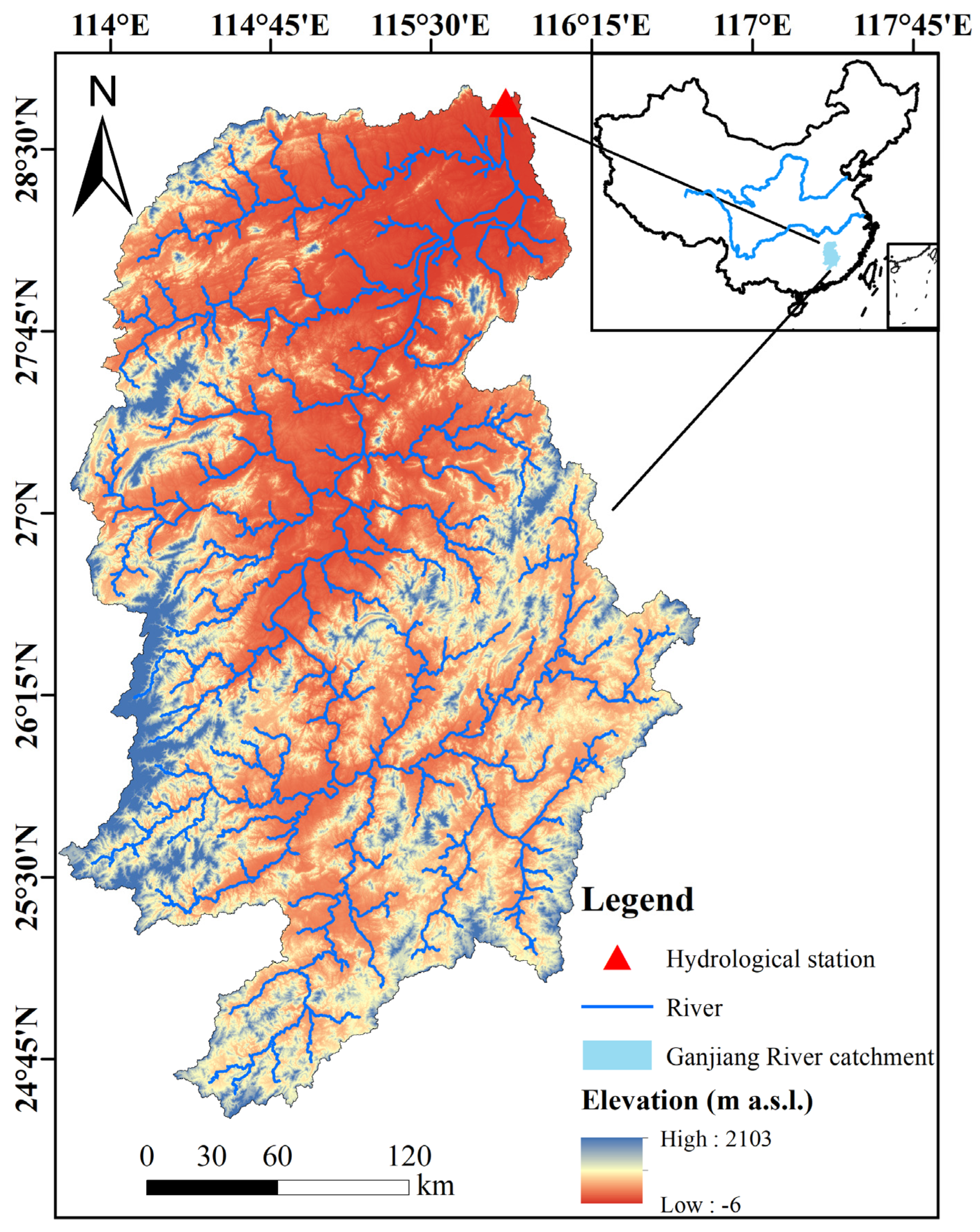
The Ganjiang River, which originates from Huangzhuling in Wuyi Mountain, is the main river in the Poyang Lake basin, accounting for 51% of its area (see Figure 2). The basin is located between the longitudes 113°45′–114°45′ E and latitudes 25°55′–26°35′ N and has a total drainage area of 80,948 km2, all within Jiangxi Province. The landscape is mainly mountainous and hilly, with a terraced distribution from the south to the north and an altitude of 23–2103 m above sea level. The basin belongs to the subtropical humid monsoon climate, characterized by abundant rainfall, while the spatiotemporal distribution of precipitation is unevenly affected by the terrain and monsoon, with 50% of the precipitation concentrated from April to June. The average annual rainfall, potential evapotranspiration, and runoff are about 1550 mm, 1070 mm, and 870 mm, respectively [50]. According to local government documents, April to September is defined as the flood season of the basin.
The monthly runoff data of Waizhou Station are collected from the local hydrological departments with time ranges from 1957 to 2016. Likewise, Atmospheric circulation indexes consist of 88 atmospheric circulation indexes, 26 sea temperature indexes, and 16 other indexes provided by the National Climate Center of China Meteorological Administration (http://cmdp.ncc-cma.net/Monitoring/cn_indexes_130.php accessed on 4 December 2023). Note that the first 80% of the above sequence data are used for training, while the last 20% are used for verifying.

3.2. Monthly Runoff from the VMD Decomposition

The decomposition effect of VMD is largely influenced by the number of mode decompositions (K), and the subsequent prediction effect will be affected if the selecting value of K is unreasonable. In general, the appropriate K value can be preliminarily selected according to the distribution of center frequency under different modes. To further determine K, the correlation of the decomposed adjacent mode components is analyzed, as shown in Table 1. In the table, rn–m represents the correlation coefficient of the decomposed nth mode and the mth mode. It can be seen that when the K is less than 6 or larger than 8, the correlation coefficients of adjacent modal components fluctuate greatly, which indicates that the mode component is stacked, leading to the over-decomposition of the runoff signal. When K is between 6 and 8, the correlation coefficient of the adjacent mode components is stable and less than 0.2, and each mode shows the runoff signal characteristics of the corresponding central frequency. Therefore, the K value of Waizhou station is selected as 8.
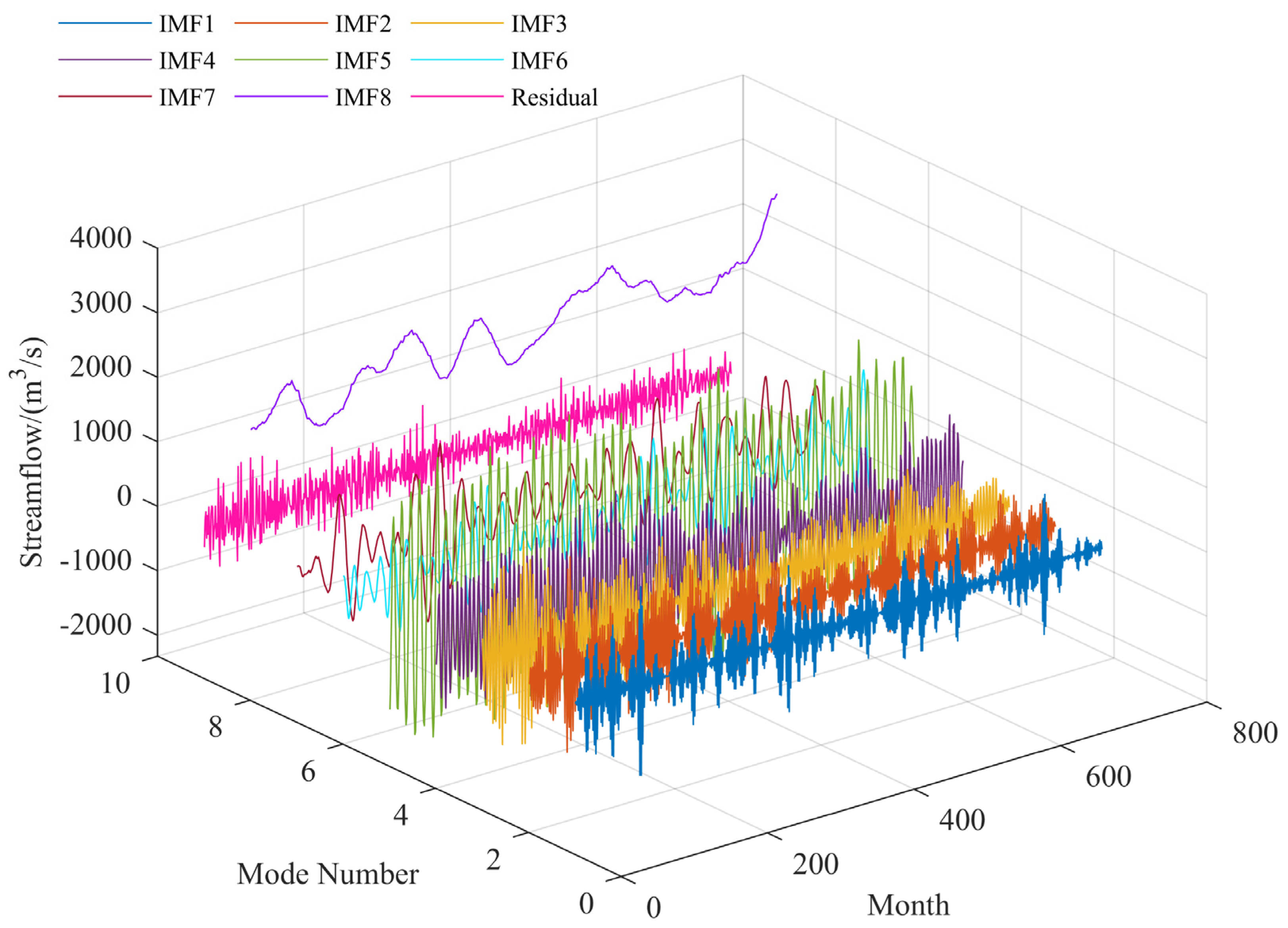
The results of monthly runoff from Waizhou station after VMD decomposition are shown in Figure 3. The original monthly runoff series is decomposed into eight stationary components (IMF) and a residual term representing the trend, which not only reduces the noise but also helps the model identify the internal transformation law of the runoff series.

4. Results and Discussion

4.1. Determining Forecasting Factors and Model Parameter

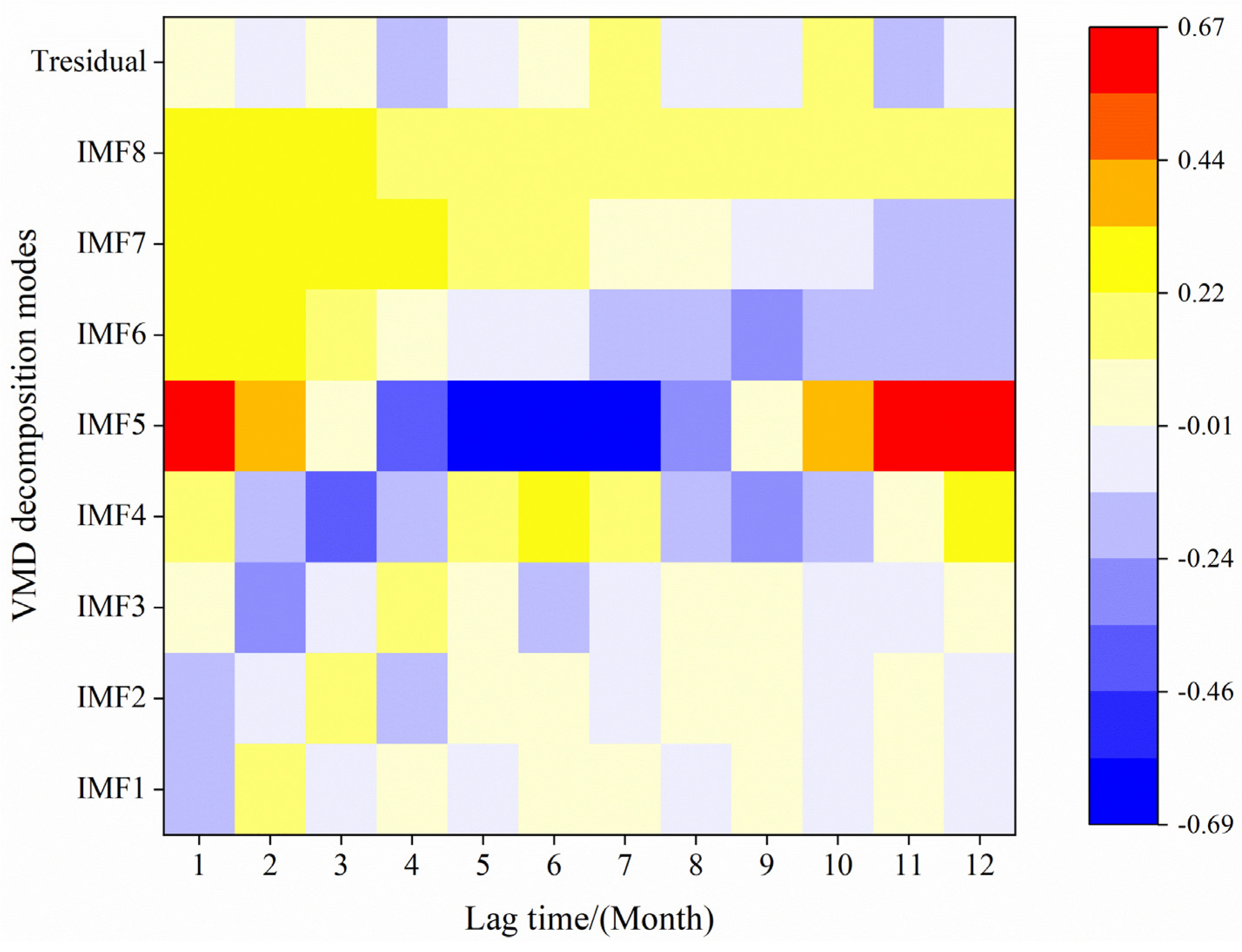
At present, there is no specific principle on how to screen the input elements of machine learning models, and the correlation coefficient method is commonly used in previous studies [30,51]. However, considering VMD decomposition causing the change in runoff interannual variation law, the optimal value of lag time (L) is selected according to the value of correlation coefficients (r) between the IMF and the original runoff series. Taking L equal to 1 month as an example, Figure 4 shows the value of r between each IMF and the original runoff series under different L; red and yellow shading indicate a good related degree, and blue shading represents poor. It can be seen that when the mode number is larger than 5, the value of r decreases as L increases, and when the mode number is less than 5, the value of r slightly fluctuates; meanwhile, the r of IMF5 presents a decrease and then an increase trend with increasing L. Additionally, to further determine the optimal value of L, the sum of r is obtained by each IMF in the same L, and the value of L is finally determined as 1 by selecting the L corresponding to the maximum sum of r.
Similarly, the optimal value of lag time (L) is determined according to the value of r between atmospheric circulation indexes and the original runoff series. In order to select circulation indexes that are as strongly correlated with monthly runoff as much as possible, the top 1% of r among circulation indexes that pass the 0.01 significance test is selected as model additional input factors. It can be found from Table 2 that L is mainly equal to 7 and 8, and the r of North African Subtropical High Ridge Position Indexes, Indian Subtropical High Ridge Position Indexes, and Western Pacific Subtropical High Ridge Position Indexes separately are the top three, which confirms previous studies about the effect of atmospheric circulation indexes on moisture transport in eastern China [52]. Additionally, considering that excessive input factors in the machine learning model will cause an overfitting phenomenon, the PCA method is used to reduce the input dimensions of the above circulation indexes. The ranking of variance contribution for the partial components is shown in Table 3. In general, the greater the variance contribution of the principal component, the more information on the selected factor. It should be noted that the variance contribution of the first principal component reaches 85.42%, indicating that it contains most of the information of the selected circulation indexes. According to the cumulative contribution rate threshold set in Section 2.4, the first two principal components are finally determined as the additional forecasting factors.

4.2. Effect of VMD Decomposition on Runoff Prediction of LSTM Model

To investigate the influence of the VMD decomposition method on the runoff prediction results of the LSTM model, the single LSTM model and the VMD-LSTM model are used to predict the monthly runoff of Waizhou hydrographic stations. The runoff prediction results of different forecast periods are shown in Table 4.
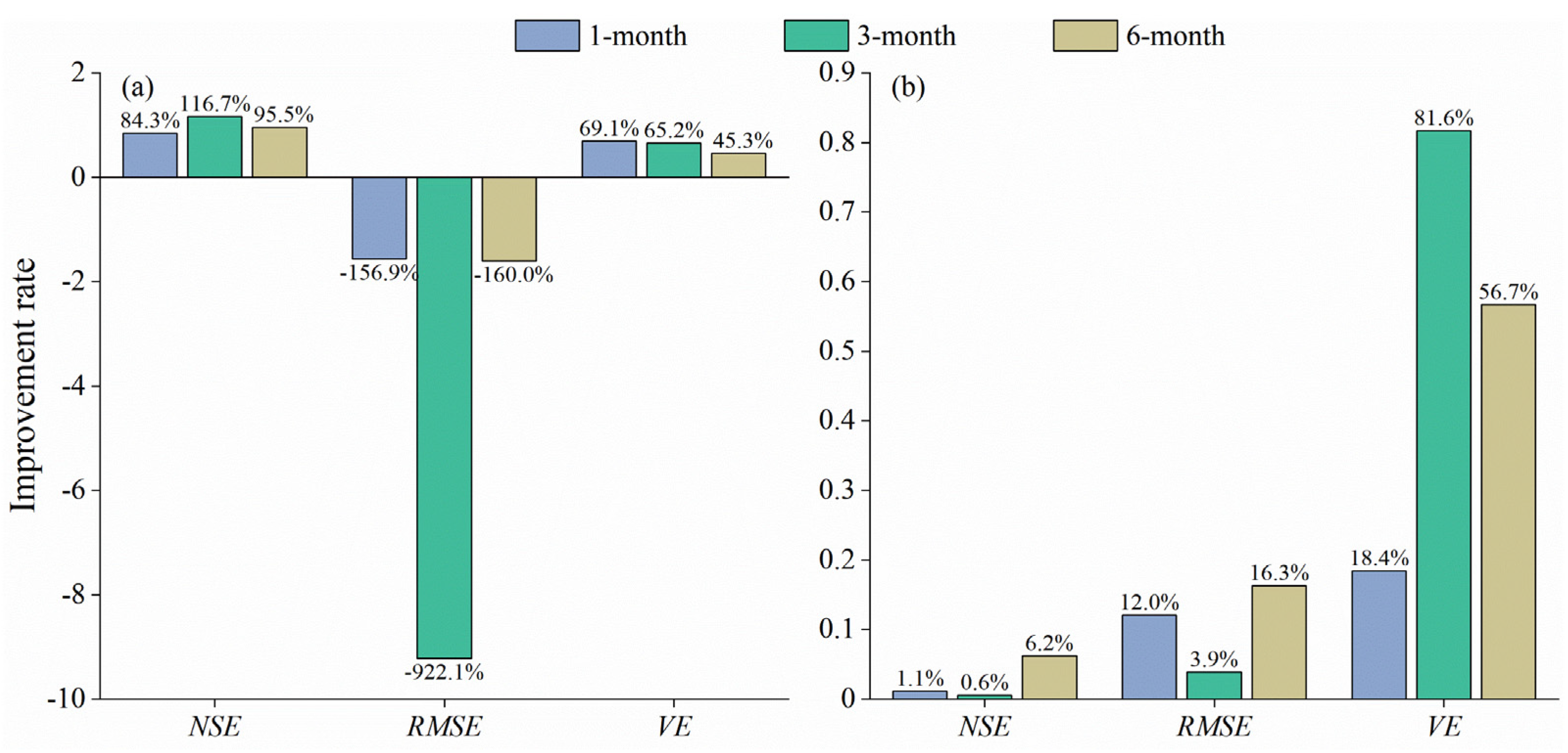
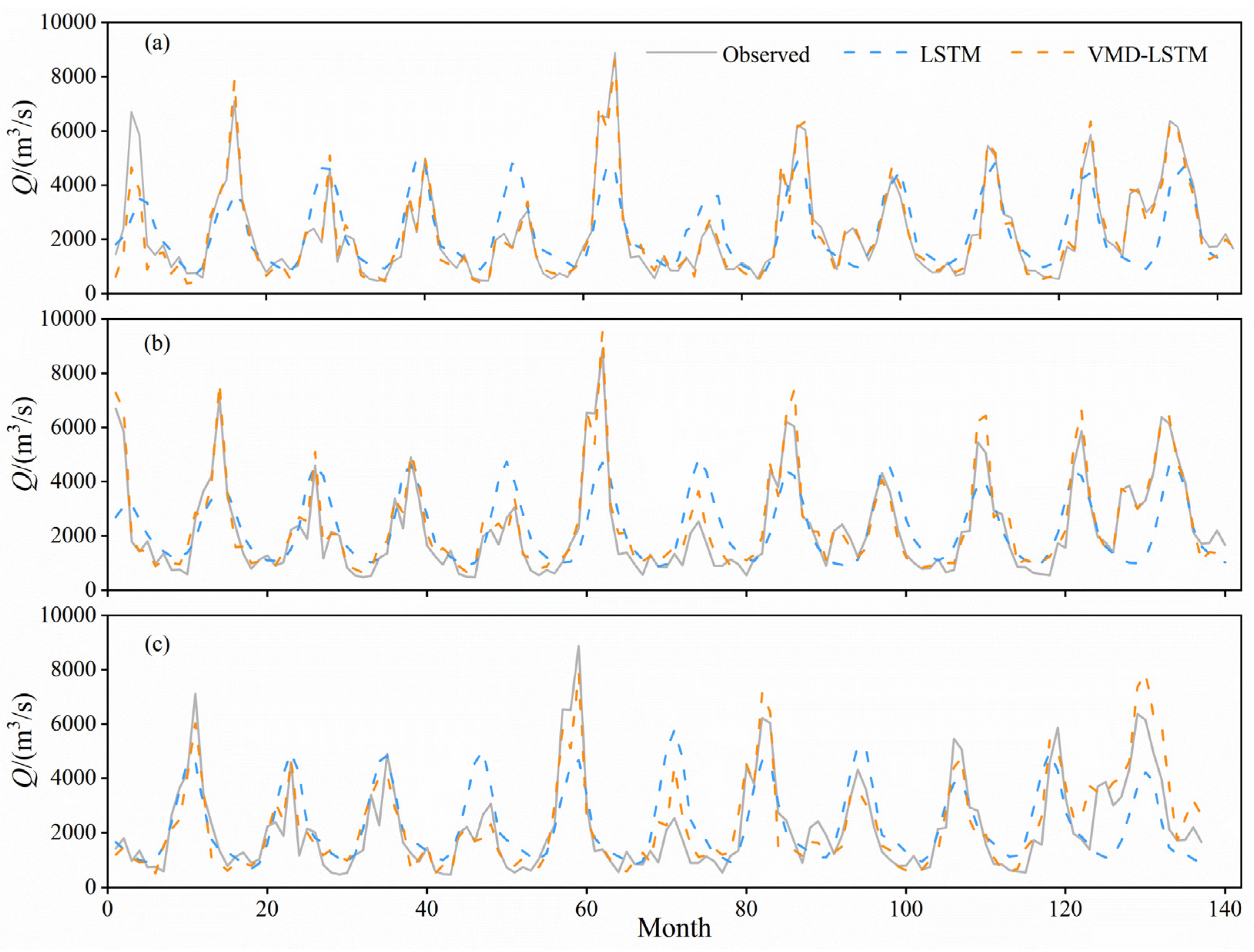
The VMD-LSTM model demonstrates significant improvements over the single LSTM model. Specifically, it increases the NSE by 0.404–0.501 and decreases the RMSE by 589–842 m3/s. This suggests that the VMD method significantly enhances the predictive performance of the single LSTM model. Figure 5a further shows the performance of the single LSTM model and the VMD-LSTM model in predicting the monthly runoff for different forecasting periods. A great improvement occurs in predicting the monthly runoff for 3 months, with the NSE increasing by 116.7% and RMSE decreasing by 922.1%. However, it is worth noting that the VE obtained by the VMD-LSTM model increases by 45.3–69.1% compared with the single LSTM model. The reason can be inferred from Figure 6, that the single LSTM model’s overestimation of medium and low flow compensates for its underestimation of high flow.
Additionally, the prediction accuracy of all models gradually degenerates as the forecast period prolongs, while the VMD-LSTM model degenerates less; for example, the NSE of the LSTM and VMD-LSTM model decreases by 18.1% and 13.2% in the foresight period from 1 month to 6 months, respectively. In comparison, when the forecast period increases from 1 month to 3 months, the NSE of the VMD-LSTM model shows no significant change, indicating that the VMD decomposition method not only improves the prediction performance of the LSTM model but also extends the forecast period in a certain extent. As shown in Figure 6, the prediction performance of the VMD-LSTM model for high flow is significantly better than that of the single LSTM model in the same forecast period. It is worth noting that the NSE of the VMD-LSTM is greater than 0.8, as the forecast period is prolonged, which further explains that the prediction ability improvement of the LSTM model by the VMD decomposition method is mainly reflected in the improvement of the prediction of the high flow.

4.3. Effect of Considering Atmospheric Circulation on Runoff Prediction of LSTM Model

The above research shows that the VMD-LSTM model can simulate the runoff with a lead time of 1, 3 and 6 months more accurately than the single LSTM model. To further enhance the prediction performance, the first two principal components of the atmospheric circulation indexes screened by the PCA method are used as the additional input of the VMD-LSTM model for the simulation of the monthly runoff with a lead time of 1, 3 and 6 months. The runoff prediction results for different forecast periods before and after integrating atmospheric circulation indexes are shown in Table 5. Different from only considering the VMD method, all metrics obtained by the VMD-PCA-LSTM model are better than the VMD-LSTM model, which means that considering the atmospheric circulation indexes as the forecasting factors can comprehensively enhance the prediction performance of the VMD-LSTM model.
Figure 5b further shows the prediction performance of the VMD-LSTM and VMD-PCA-LSTM models for different forecasting periods. It can be found that the improvement degree of the VMD-LSTM model after integrating atmospheric circulation indexes becomes more significant as the forecast period prolongs, particularly when the forecast period is 6 months, the NSE and RMSE have the most significant improvement with increasing by 6.2% and 16.3%, respectively. The reason may be that the long-term continuous influence of atmospheric circulation on regional climate leads to the fact that the atmospheric circulation indexes of the previous period still affect the climate for a long time in the future, and then affect the runoff through the water cycle process. Therefore, with the increase in the forecast period, the effect of historical runoff gradually weakens, and the prediction performance of the model gradually decreases, while the atmospheric circulation factors still play a certain role in the runoff prediction in the following months, which makes the accuracy of the model improve more significantly with the increase in the forecast period after the integration of atmospheric circulation indexes.
Figure 7 intuitively displays the forecast performance of the VMD-LSTM and VMD-PCA-LSTM models in different forecast periods. When the forecast period is one month, all models can predict well the future change trend of runoff. With the increase in the forecast period, the predicted runoff of the VMD-PCA-LSTM model still maintains a high degree of correspondence with the observed, while the predicted runoff of the VMD-LSTM model has a significant deviation, mainly manifesting as an overestimation of high flow prediction. Due to the small number of samples at the high flow, the accurate prediction of high flow becomes a difficult problem in runoff prediction. The results indicate that adding atmospheric circulation indexes to the model input can effectively solve the problem of low prediction accuracy at high flow caused by a small number of samples.

4.4. Performance of Runoff Prediction in Flood and Non-Flood Season

As a result of the uneven spatiotemporal distribution of precipitation in the basin, issues such as flood disasters, drought, and mismatch between water supply and demand have become progressively prominent. Therefore, the accurate prediction of runoff in flood and non-flood seasons can provide a scientific basis for effectively reducing the risk of flood damage and mitigating the mismatch between water supply and demand.
The prediction results for three models during different forecast periods are displayed in Figure 8. It is quite obvious that the LSTM model slightly overestimates the low flow and strongly underestimates the high flow at all times, which is resolved by the introduction of the VMD method, and the forecast period equaling 1 month is especially significantly improved, while the difference between the VMD-LSTM and VMD-PCA-LSTM models is not obvious. Table 6 demonstrates the runoff prediction results of the VMD-LSTM and VMD-PCA-LSTM models. Compared with the VMD-LSTM model, the performance of the VMD-PCA-LSTM model is better in flood season and degrades in non-flood season, with the r and RMSE decreased by 1.7–5.8% and increased 0.7–6.5% in non-flood season and increased by 1.7–5.8% and decreased 0.7–25.1% in flood season, respectively. The results indicate that consideration of atmospheric circulation indexes is not a comprehensive improvement of the model’s runoff prediction ability, but rather focuses only on the flood season, particularly for high flows.
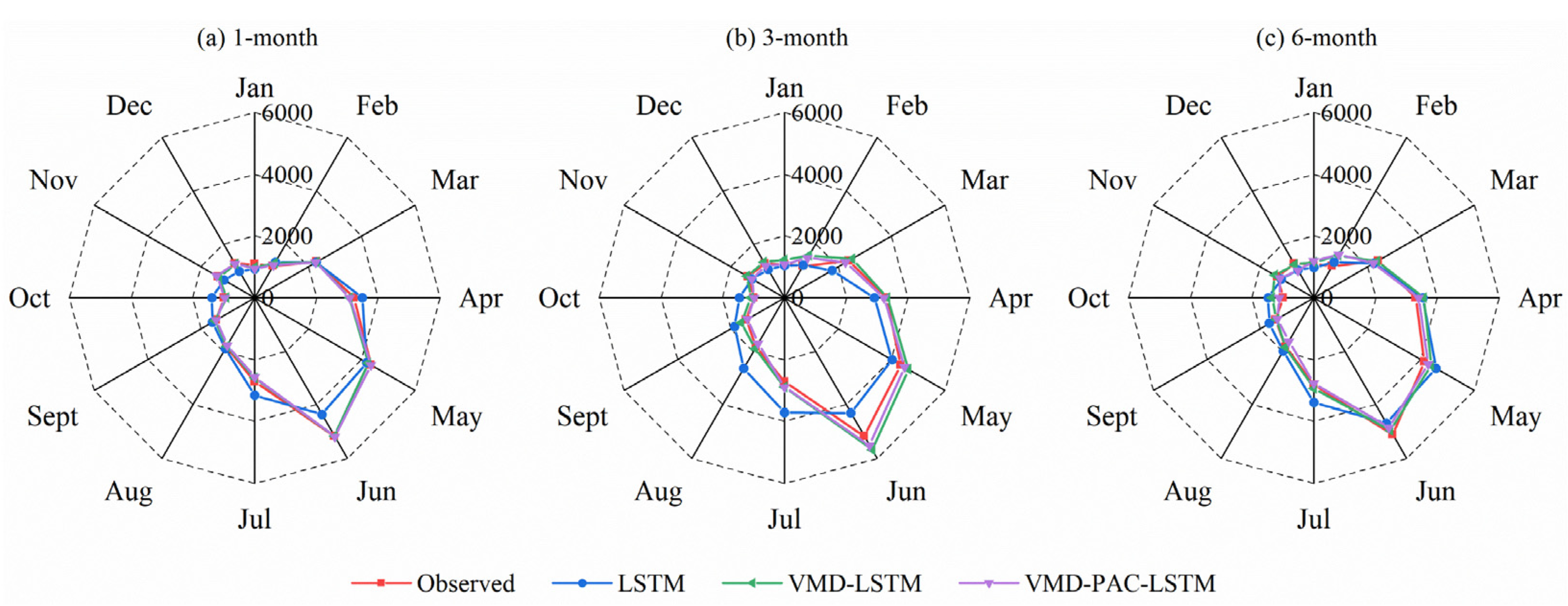
Figure 9 presents the results of predicted monthly mean runoff in different forecast periods. There is no significant difference between all models from November to February, and only considering VMD decomposition can improve the LSTM model accuracy of other monthly runoff predictions, while the VMD-PCA-LSTM model slightly improves the VMD-LSTM model overestimation of runoff in all forecast period. In addition, the VMD-LSTM and VMD-PCA-LSTM models have good robustness with increasing forecast periods compared to the LSTM model.

4.5. Discussion

This study uses an LSTM model coupled with VMD and PCA methods to predict the monthly runoff and finds that the hybrid model can enhance the model’s predictive accuracy, particularly during the flood season. This is consistent with previous studies that reported an improvement based on the deep learning and decomposition technique for the runoff prediction [53,54]. It is worth noting that considering the structural differences of the model, different results can be obtained under different deep learning models. For example, Li et al. [55] found that the prediction results of back propagation neural network (BPNN), SVM and LSTM had significant differences, and the performance of the LSTM model was the best, especially for the peak flow forecasting. Meanwhile, many researchers often use the LSTM model for hydrological simulation and prediction. Therefore, our study only tests the effect of the LSTM model under VMD and PCA methods and does not further explore the effects of different models.
On the other hand, with the rapid development of decomposition methods, new methods such as the wavelet packet decomposition (WPD), complete ensemble empirical mode decomposition with adaptive noise (CEEMDAN) and singular spectrum analysis (SSA) demonstrate some advantages in medium- and long-term term runoff forecasting [56,57]. However, it cannot simply be concluded that new methods will always produce the best simulations under all conditions. Wang et al. [58] pointed out that selecting an appropriate data pre-processing method based on the specific characteristics of the study area can lead to more accurate prediction results. Therefore, further research is needed on the application of various decomposition techniques in the Ganjiang River Basin.
In addition, the goodness of the result for screening the input factors also influences the model performance. Global sensitivity analysis is a feasible method for selecting medium- and long-term runoff prediction factors based on physical causes, while it is not computationally efficient for complex models and large amounts of data [59]. The correlation coefficient method used in this study is simple and effective based on statistical relationships, but it still requires a subjective setting of the threshold [30]. Recently, attention mechanisms have shown great application potential in identifying key input factors of runoff prediction by automatically assigning weights to all factors [13]. Consequently, it is necessary to further study the LSTM model of coupled attention mechanism and advanced optimization algorithm in the future.

5. Conclusions

This study introduces a hybrid machine learning model built upon the LSTM model coupled with the VMD and PCA for monthly runoff prediction. The VMD decomposition was employed to reduce the noise in the runoff series, while correlation analysis determined the lag time for each IMF and the atmospheric circulation indexes. The PCA method was then utilized to select the forecasting factors from the atmospheric circulation indexes. Finally, the Bayesian optimization algorithm was used to optimize the LSTM network parameters. The constructed hybrid LSTM model was applied to the Waizhou station, considering lead times of 1, 3 and 6 months, aiming ultimately to investigate the impact of VMD decomposition and the inclusion of atmospheric circulation indexes on the runoff prediction accuracy of the LSTM model. The main conclusions are presented below:
(1)
For Waizhou station, the number of mode decomposition K is 8, with lag time (L) equaling 1 month. The L of atmospheric circulation indexes is mainly equal to 7 and 8, and the r of North African Subtropical High Ridge Position Indexes, Indian Subtropical High Ridge Position Indexes, and Western Pacific Subtropical High Ridge Position Indexes separately are the top three. The first two principal components are selected as the forecasting factors from the above atmospheric circulation indexes by the PCA method.
(2)
The VMD decomposition method can significantly improve the prediction accuracy of the single LSTM model, especially concentrating on the prediction of high flow during the flood and non-flood seasons, and the improvement rate of NSE and RMSE are 84.3–116.7% and 156.9–922.1% except the VE. Additionally, as the forecast period increases, the prediction accuracy of the VMD-LSTM model degenerates less, indicating that the VMD-LSTM model has good robustness. Only considering VMD decomposition can improve the LSTM model accuracy of other monthly runoff predictions except from November to February, which is not significantly different from the VMD-PCA-LSTM model.
(3)
Considering the atmospheric circulation indexes as the forecasting factors, compared to the VMD-LSTM model, significantly enhances prediction accuracy in high flow caused by a small number of samples, especially the decrease in VE of up to 81.6%. With the increase in the forecast period, the improvement after integrating atmospheric circulation indexes becomes more significant, especially when the forecast period is 6 months. The NSE and RMSE have the most significant improvement increasing by 6.2% and 16.3%. However, it is worth noting that the VMD-PCA-LSTM model does not offer a comprehensive enhancement over the VMD-LSTM model in all periods, but rather focuses only on the flood season, particularly for high flows.

Author Contributions

Conceptualization, W.W., S.T. and J.Z.; Data curation, W.W and S.T.; Formal analysis, S.T. and J.Z.; Funding acquisition, X.Y.; Investigation, D.L.; Methodology, W.W., S.T. and J.Z.; Supervision, X.G. and J.H.; Visualization, S.T. and J.Z.; Writing—original draft, W.W., S.T. and J.Z.; Writing—review and editing, W.W., S.T., J.Z. and X.Y. All authors have read and agreed to the published version of the manuscript.

Funding

This research was funded by the National Key Research and Development Program of China (2023YFC3206804), the National Natural Science Foundation of China (52394234), and the Jiangxi Province “Science and Technology + Water Conservancy” Joint Plan Project (2022KSG01006).

Data Availability Statement

Data are available from the corresponding author upon reasonable request.

Acknowledgments

The anonymous reviewers and the editor are thanked for providing insightful and detailed reviews that greatly improved the manuscript.

Conflicts of Interest

The authors declare no conflicts of interest.

References

  1. Niu, W.-J.; Feng, Z.-K. Evaluating the performances of several artificial intelligence methods in forecasting daily streamflow time series for sustainable water resources management. Sustain. Cities Soc. 2021, 64, 102562. [Google Scholar] [CrossRef]
  2. Feng, Z.-K.; Niu, W.-J.; Tang, Z.-Y.; Jiang, Z.-Q.; Xu, Y.; Liu, Y.; Zhang, H.-R. Monthly runoff time series prediction by variational mode decomposition and support vector machine based on quantum-behaved particle swarm optimization. J. Hydrol. 2020, 583, 124627. [Google Scholar] [CrossRef]
  3. Tikhamarine, Y.; Souag-Gamane, D.; Ahmed, A.N.; Sammen, S.S.; Kisi, O.; Huang, Y.F.; El-Shafie, A. Rainfall-runoff modelling using improved machine learning methods: Harris hawks optimizer vs. particle swarm optimization. J. Hydrol. 2020, 589, 125133. [Google Scholar] [CrossRef]
  4. Akbarian, M.; Saghafian, B.; Golian, S. Monthly streamflow forecasting by machine learning methods using dynamic weather prediction model outputs over Iran. J. Hydrol. 2023, 620, 129480. [Google Scholar] [CrossRef]
  5. Dung, N.B.; Long, N.Q.; Goyal, R.; An, D.T.; Minh, D.T. The Role of Factors Affecting Flood Hazard Zoning Using Analytical Hierarchy Process: A Review. Earth Syst. Environ. 2022, 6, 697–713. [Google Scholar] [CrossRef]
  6. Stergiadi, M.; Di Marco, N.; Avesani, D.; Righetti, M.; Borga, M. Impact of Geology on Seasonal Hydrological Predictability in Alpine Regions by a Sensitivity Analysis Framework. Water 2020, 12, 2255. [Google Scholar] [CrossRef]
  7. Yang, Q.; Zhang, H.; Wang, G.; Luo, S.; Chen, D.; Peng, W.; Shao, J. Dynamic runoff simulation in a changing environment: A data stream approach. Environ. Model. Softw. 2019, 112, 157–165. [Google Scholar] [CrossRef]
  8. Deng, C.; Wang, W. Runoff Predicting and Variation Analysis in Upper Ganjiang Basin under Projected Climate Changes. Sustainability 2019, 11, 5885. [Google Scholar] [CrossRef]
  9. Chen, X.; Zhang, K.; Luo, Y.; Zhang, Q.; Zhou, J.; Fan, Y.; Huang, P.; Yao, C.; Chao, L.; Bao, H. A distributed hydrological model for semi-humid watersheds with a thick unsaturated zone under strong anthropogenic impacts: A case study in Haihe River Basin. J. Hydrol. 2023, 623, 129765. [Google Scholar] [CrossRef]
  10. Kirsta, Y.B.; Troshkova, I.A. High-Performance Forecasting of Spring Flood in Mountain River Basins with Complex Landscape Structure. Water 2023, 15, 1080. [Google Scholar] [CrossRef]
  11. Xu, Y.; Hu, C.; Wu, Q.; Jian, S.; Li, Z.; Chen, Y.; Zhang, G.; Zhang, Z.; Wang, S. Research on particle swarm optimization in LSTM neural networks for rainfall-runoff simulation. J. Hydrol. 2022, 608, 127553. [Google Scholar] [CrossRef]
  12. Meng, J.; Dong, Z.; Shao, Y.; Zhu, S.; Wu, S. Monthly Runoff Forecasting Based on Interval Sliding Window and Ensemble Learning. Sustainability 2023, 15, 100. [Google Scholar] [CrossRef]
  13. Han, D.Y.; Liu, P.; Xie, K.; Li, H.; Xia, Q.; Cheng, Q.; Wang, Y.B.; Yang, Z.K.; Zhang, Y.J.; Xia, J. An attention-based LSTM model for long-term runoff forecasting and factor recognition. Environ. Res. Lett. 2023, 18, 13. [Google Scholar] [CrossRef]
  14. Kim, T.; Yang, T.; Gao, S.; Zhang, L.; Ding, Z.; Wen, X.; Gourley, J.J.; Hong, Y. Can artificial intelligence and data-driven machine learning models match or even replace process-driven hydrologic models for streamflow simulation?: A case study of four watersheds with different hydro-climatic regions across the CONUS. J. Hydrol. 2021, 598, 126423. [Google Scholar] [CrossRef]
  15. Zhang, S.; Gan, T.Y.; Bush, A.B.G.; Zhang, G. Evaluation of the impact of climate change on the streamflow of major pan-Arctic river basins through machine learning models. J. Hydrol. 2023, 619, 129295. [Google Scholar] [CrossRef]
  16. Zang, S.; Li, Z.; Zhang, K.; Yao, C.; Liu, Z.; Wang, J.; Huang, Y.; Wang, S. Improving the flood prediction capability of the Xin’anjiang model by formulating a new physics-based routing framework and a key routing parameter estimation method. J. Hydrol. 2021, 603, 126867. [Google Scholar] [CrossRef]
  17. Abbaspour, K.C.; Rouholahnejad, E.; Vaghefi, S.; Srinivasan, R.; Yang, H.; Kløve, B. A continental-scale hydrology and water quality model for Europe: Calibration and uncertainty of a high-resolution large-scale SWAT model. J. Hydrol. 2015, 524, 733–752. [Google Scholar] [CrossRef]
  18. Behrangi, A.; Khakbaz, B.; Jaw, T.C.; AghaKouchak, A.; Hsu, K.; Sorooshian, S. Hydrologic evaluation of satellite precipitation products over a mid-size basin. J. Hydrol. 2011, 397, 225–237. [Google Scholar] [CrossRef]
  19. Avesani, D.; Galletti, A.; Piccolroaz, S.; Bellin, A.; Majone, B. A dual-layer MPI continuous large-scale hydrological model including Human Systems. Environ. Model. Softw. 2021, 139, 105003. [Google Scholar] [CrossRef]
  20. Nazemi, A.; Wheater, H.S. On inclusion of water resource management in Earth system models—Part 1: Problem definition and representation of water demand. Hydrol. Earth Syst. Sci. 2015, 19, 33–61. [Google Scholar] [CrossRef]
  21. Bozorg-Haddad, O.; Zarezadeh-Mehrizi, M.; Abdi-Dehkordi, M.; Loáiciga, H.A.; Mariño, M.A. A self-tuning ANN model for simulation and forecasting of surface flows. Water Resour. Manag. 2016, 30, 2907–2929. [Google Scholar] [CrossRef]
  22. Hagen, J.S.; Leblois, E.; Lawrence, D.; Solomatine, D.; Sorteberg, A. Identifying major drivers of daily streamflow from large-scale atmospheric circulation with machine learning. J. Hydrol. 2021, 596, 126086. [Google Scholar] [CrossRef]
  23. Liu, P.; Wang, J.; Sangaiah, A.K.; Xie, Y.; Yin, X. Analysis and Prediction of Water Quality Using LSTM Deep Neural Networks in IoT Environment. Sustainability 2019, 11, 2058. [Google Scholar] [CrossRef]
  24. Yu, Q.; Jiang, L.; Wang, Y.; Liu, J. Enhancing streamflow simulation using hybridized machine learning models in a semi-arid basin of the Chinese loess Plateau. J. Hydrol. 2023, 617, 129115. [Google Scholar] [CrossRef]
  25. Wang, X.; Sun, W.; Lu, F.; Zuo, R. Combining Satellite Optical and Radar Image Data for Streamflow Estimation Using a Machine Learning Method. Remote Sens. 2023, 15, 5184. [Google Scholar] [CrossRef]
  26. Kim, T.; Shin, J.Y.; Kim, H.; Heo, J.H. Ensemble-Based Neural Network Modeling for Hydrologic Forecasts: Addressing Uncertainty in the Model Structure and Input Variable Selection. Water Resour. Res. 2020, 56, 19. [Google Scholar] [CrossRef]
  27. Bedi, J. Transfer learning augmented enhanced memory network models for reference evapotranspiration estimation. Knowl.-Based Syst. 2022, 237, 107717. [Google Scholar] [CrossRef]
  28. Xu, L.; Yu, H.; Chen, Z.; Du, W.; Chen, N.; Huang, M. Hybrid Deep Learning and S2S Model for Improved Sub-Seasonal Surface and Root-Zone Soil Moisture Forecasting. Remote Sens. 2023, 15, 3410. [Google Scholar] [CrossRef]
  29. Castangia, M.; Grajales, L.M.M.; Aliberti, A.; Rossi, C.; Macii, A.; Macii, E.; Patti, E. Transformer neural networks for interpretable flood forecasting. Environ. Model. Softw. 2023, 160, 105581. [Google Scholar] [CrossRef]
  30. Yao, Z.; Wang, Z.; Wang, D.; Wu, J.; Chen, L. An ensemble CNN-LSTM and GRU adaptive weighting model based improved sparrow search algorithm for predicting runoff using historical meteorological and runoff data as input. J. Hydrol. 2023, 625, 129977. [Google Scholar] [CrossRef]
  31. Song, P.; Liu, W.; Sun, J.; Wang, C.; Kong, L.; Nong, Z.; Lei, X.; Wang, H. Annual Runoff Forecasting Based on Multi-Model Information Fusion and Residual Error Correction in the Ganjiang River Basin. Water 2020, 12, 2086. [Google Scholar] [CrossRef]
  32. Zhao, X.; Lv, H.; Lv, S.; Sang, Y.; Wei, Y.; Zhu, X. Enhancing robustness of monthly streamflow forecasting model using gated recurrent unit based on improved grey wolf optimizer. J. Hydrol. 2021, 601, 126607. [Google Scholar] [CrossRef]
  33. Fang, W.; Huang, S.; Ren, K.; Huang, Q.; Huang, G.; Cheng, G.; Li, K. Examining the applicability of different sampling techniques in the development of decomposition-based streamflow forecasting models. J. Hydrol. 2019, 568, 534–550. [Google Scholar] [CrossRef]
  34. Zuo, G.G.; Luo, J.G.; Wang, N.; Lian, Y.N.; He, X.X. Two-stage variational mode decomposition and support vector regression for streamflow forecasting. Hydrol. Earth Syst. Sci. 2020, 24, 5491–5518. [Google Scholar] [CrossRef]
  35. Wang, W.-C.; Chau, K.-W.; Xu, D.-M.; Chen, X.-Y. Improving Forecasting Accuracy of Annual Runoff Time Series Using ARIMA Based on EEMD Decomposition. Water Resour. Manag. 2015, 29, 2655–2675. [Google Scholar] [CrossRef]
  36. Zuo, G.; Luo, J.; Wang, N.; Lian, Y.; He, X. Decomposition ensemble model based on variational mode decomposition and long short-term memory for streamflow forecasting. J. Hydrol. 2020, 585, 124776. [Google Scholar] [CrossRef]
  37. Kirono, D.G.C.; Chiew, F.H.S.; Kent, D.M. Identification of best predictors for forecasting seasonal rainfall and runoff in Australia. Hydrol. Process. 2010, 24, 1237–1247. [Google Scholar] [CrossRef]
  38. Chavasse, D.I.; Seoane, R.S. Assessing and predicting the impact of El Nino southern oscillation (ENSO) events on runoff from the Chopim River basin, Brazil. Hydrol. Process. 2009, 23, 3261–3266. [Google Scholar] [CrossRef]
  39. Champagne, O.; Arain, M.A.; Coulibaly, P. Atmospheric circulation amplifies shift of winter streamflow in southern Ontario. J. Hydrol. 2019, 578, 124051. [Google Scholar] [CrossRef]
  40. Yan, X.; Chang, Y.; Yang, Y.; Liu, X. Monthly runoff prediction using modified CEEMD-based weighted integrated model. J. Water Clim. Change 2020, 12, 1744–1760. [Google Scholar] [CrossRef]
  41. Mostaghimzadeh, E.; Ashrafi, S.M.; Adib, A.; Geem, Z.W. A long lead time forecast model applying an ensemble approach for managing the great Karun multi-reservoir system. Appl. Water Sci. 2023, 13, 124. [Google Scholar] [CrossRef]
  42. Dragomiretskiy, K.; Zosso, D. Variational Mode Decomposition. IEEE Trans. Signal Process. 2014, 62, 531–544. [Google Scholar] [CrossRef]
  43. Zhang, X.; Liu, F.; Yin, Q.; Qi, Y.; Sun, S. A runoff prediction method based on hyperparameter optimisation of a kernel extreme learning machine with multi-step decomposition. Sci. Rep. 2023, 13, 19341. [Google Scholar] [CrossRef]
  44. Jolliffe, I.T.; Cadima, J. Principal component analysis: A review and recent developments. Philos. Trans. R. Soc. A-Math. Phys. Eng. Sci. 2016, 374, 16. [Google Scholar] [CrossRef]
  45. Hochreiter, S.; Schmidhuber, J. Long Short-Term Memory. Neural Comput. 1997, 9, 1735–1780. [Google Scholar] [CrossRef]
  46. Thiemann, M.; Trosset, M.; Gupta, H.; Sorooshian, S. Bayesian recursive parameter estimation for hydrologic models. Water Resour. Res. 2001, 37, 2521–2535. [Google Scholar] [CrossRef]
  47. Kratzert, F.; Klotz, D.; Brenner, C.; Schulz, K.; Herrnegger, M. Rainfall-runoff modelling using Long Short-Term Memory (LSTM) networks. Hydrol. Earth Syst. Sci. 2018, 22, 6005–6022. [Google Scholar] [CrossRef]
  48. Ling, H.; Xu, H.; Shi, W.; Zhang, Q. Regional climate change and its effects on the runoff of Manas River, Xinjiang, China. Environ. Earth Sci. 2011, 64, 2203–2213. [Google Scholar] [CrossRef]
  49. Mo, R.; Xu, B.; Zhong, P.-A.; Dong, Y.; Wang, H.; Yue, H.; Zhu, J.; Wang, H.; Wang, G.; Zhang, J. Long-term probabilistic streamflow forecast model with “inputs–structure–parameters” hierarchical optimization framework. J. Hydrol. 2023, 622, 129736. [Google Scholar] [CrossRef]
  50. Deng, C.; Yin, X.; Zou, J.; Wang, M.; Hou, Y. Assessment of the impact of climate change on streamflow of Ganjiang River catchment via LSTM-based models. J. Hydrol. Reg. Stud. 2024, 52, 101716. [Google Scholar] [CrossRef]
  51. Wang, N.; Zhang, D.; Chang, H.; Li, H. Deep learning of subsurface flow via theory-guided neural network. J. Hydrol. 2020, 584, 124700. [Google Scholar] [CrossRef]
  52. Tong, X.; Yan, Z.; Xia, J.; Lou, X. Decisive Atmospheric Circulation Indices for July–August Precipitation in North China Based on Tree Models. J. Hydrometeorol. 2019, 20, 1707–1720. [Google Scholar] [CrossRef]
  53. Amini, A.; Dolatshahi, M.; Kerachian, R. Real-time rainfall and runoff prediction by integrating BC-MODWT and automatically-tuned DNNs: Comparing different deep learning models. J. Hydrol. 2024, 631, 130804. [Google Scholar] [CrossRef]
  54. Ma, K.; He, D.; Liu, S.; Ji, X.; Li, Y.; Jiang, H. Novel time-lag informed deep learning framework for enhanced streamflow prediction and flood early warning in large-scale catchments. J. Hydrol. 2024, 631, 130841. [Google Scholar] [CrossRef]
  55. Li, B.-J.; Sun, G.-L.; Liu, Y.; Wang, W.-C.; Huang, X.-D. Monthly Runoff Forecasting Using Variational Mode Decomposition Coupled with Gray Wolf Optimizer-Based Long Short-term Memory Neural Networks. Water Resour. Manag. 2022, 36, 2095–2115. [Google Scholar] [CrossRef]
  56. Seo, Y.; Kim, S.; Kisi, O.; Singh, V.P.; Parasuraman, K. River Stage Forecasting Using Wavelet Packet Decomposition and Machine Learning Models. Water Resour. Manag. 2016, 30, 4011–4035. [Google Scholar] [CrossRef]
  57. Yang, C.; Jiang, Y.; Liu, Y.; Liu, S.; Liu, F. A novel model for runoff prediction based on the ICEEMDAN-NGO-LSTM coupling. Environ. Sci. Pollut. Res. 2023, 30, 82179–82188. [Google Scholar] [CrossRef]
  58. Wang, W.-C.; Du, Y.-J.; Chau, K.-W.; Cheng, C.-T.; Xu, D.-M.; Zhuang, W.-T. Evaluating the Performance of Several Data Preprocessing Methods Based on GRU in Forecasting Monthly Runoff Time Series. Water Resour. Manag. 2024. [Google Scholar] [CrossRef]
  59. Li, H.Y.; Xie, M.; Jiang, S. Recognition method for mid- to long-term runoff forecasting factors based on global sensitivity analysis in the Nenjiang River Basin. Hydrol. Process. 2012, 26, 2827–2837. [Google Scholar] [CrossRef]
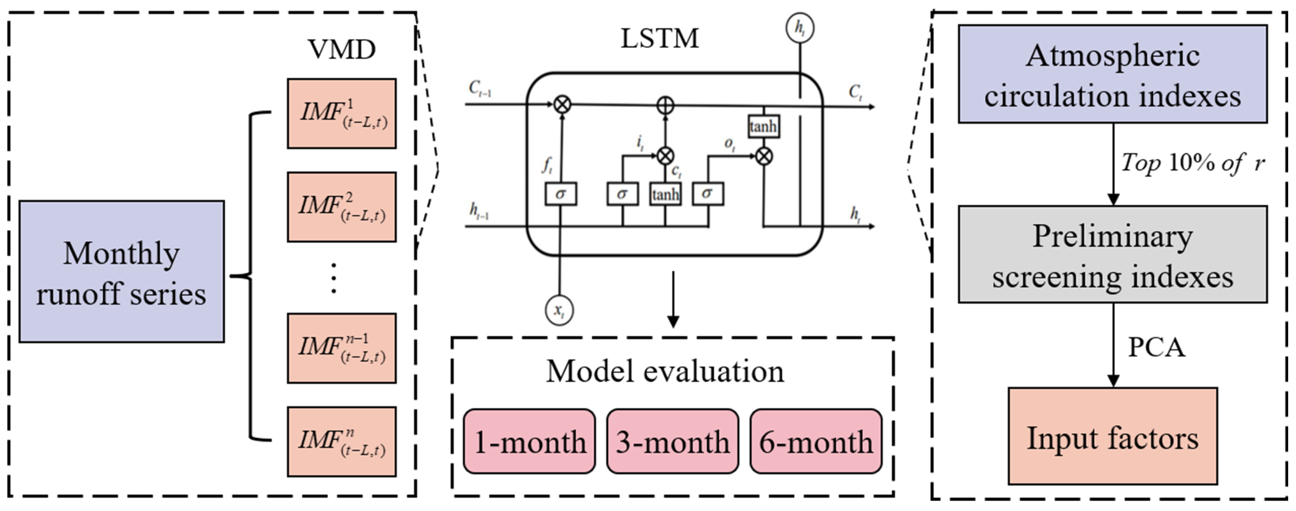
Figure 1. The process of monthly runoff prediction via the VMD-PCA-LSTM model.
Water 16 01589 g001
Figure 2. Location of the Ganjiang River Basin.
Water 16 01589 g002
Figure 3. The VMD decomposition of monthly runoff at Waizhou station.
Water 16 01589 g003
Figure 4. Heatmap of the correlation coefficient (r) between each IMF and the original runoff series under different lag times.
Water 16 01589 g004
Figure 5. Comparison of runoff prediction in different forecast periods: (a) LSTM model and VMD-LSTM model; (b) VMD-LSTM model and VMD-PCA-LSTM model.
Water 16 01589 g005
Figure 6. The monthly runoff prediction results during different forecast periods for LSTM and VMD-LSTM models: (a) 1 month; (b) 3 months; (c) 6 months.
Water 16 01589 g006
Figure 7. The monthly runoff prediction results during different forecast periods for VMD-LSTM and VMD-PAC-LSTM models: (a) 1-month; (b) 3-month; (c) 6-month.
Water 16 01589 g007
Figure 8. Comparison of predicted results for three models during different forecast periods: (ac) non-flood season; (df) flood season.
Water 16 01589 g008
Figure 9. Radar chart of the predicted and observed monthly mean runoff in different forecast periods.
Water 16 01589 g009
Table 1. Correlation coefficients of adjacent modes.
Kr1–2r2–3r3–4r4–5r5–6r6–7r7–8r8–9
20.128-------
30.0110.113------
40.0090.0710.203-----
50.0310.0350.0500.184----
60.0440.0290.0500.1740.170---
70.0760.0820.0240.0450.1700.169--
80.0920.0750.0810.0180.0420.1680.169-
90.0850.0890.0510.1530.0260.0350.1660.169
Table 2. The rank of correlation coefficient (r) between the atmospheric circulation indexes and the original runoff series in the optimal lag time.
Rank of rFactor TypeLag Time
/(Month)
6Northern Hemisphere Subtropical High Ridge Position Indexes7
3Western Pacific Subtropical High Ridge Position Indexes
10South China Sea Subtropical High Ridge Position Indexes
5Pacific Subtropical High Ridge Position Indexes
11North African-North Atlantic-North American Subtropical High Area Indexes8
13North American Subtropical High Area Indexes
9Atlantic Subtropical High Area Indexes
8North American-Atlantic Subtropical High Area Indexes
1North African Subtropical High Ridge Position Indexes
12North African-North Atlantic-North American Subtropical High Ridge Position Indexes
2Indian Subtropical High Ridge Position Indexes
7Northern Hemisphere Polar Vortex Central Intensity Indexes
4East Asian Trough Intensity Indexes
Table 3. The ranking of variance contribution for the partial components.
ComponentTotalVariance/(%)Cumulative Variance/(%)
111.1085.4285.42
20.906.9492.36
30.352.6895.04
40.171.3496.38
50.110.8397.21
60.0980.7597.96
Table 4. The performances of LSTM and VMD-LSTM model during the validation period.
Forecast PeriodModelNSERMSE/(m3/s)VE/(%)
1 monthLSTM0.5181185−0.77
VMD-LSTM0.954366−1.97
3 monthsLSTM0.43012920.76
VMD-LSTM0.9314507.81
6 monthsLSTM0.42412991.62
VMD-LSTM0.8287104.21
Table 5. Predicted results before and after integrating atmospheric circulation indexes. Note: the data on the left and right of the arrow represent the predicted results before and after integrating the atmospheric circulation indexes, respectively.
Forecast PeriodNSERMSE/(m3/s)VE/(%)
1 month0.954→0.964366→322−1.97→−1.61
3 months0.931→0.936450→4327.81→1.43
6 months0.828→0.879710→5954.21→−1.82
Table 6. Predicted results of VMD-LSTM and VMD-PCA-LSTM model for different forecast periods during the flood and non-flood seasons. Note: the data on the left and right of the arrow represent the predicted results of the VMD-LSTM and VMD-PCA-LSTM models, respectively.
SeasonForecast PeriodrRMSE/(m3/s)
non-flood season1 month0.974→0.957215→269
3 months0.940→0.923343→359
6 months0.846→0.797564→568
flood season1 month0.978→0.982469→366
3 months0.966→0.966532→491
6 months0.907→0.941833→589
Disclaimer/Publisher’s Note: The statements, opinions and data contained in all publications are solely those of the individual author(s) and contributor(s) and not of MDPI and/or the editor(s). MDPI and/or the editor(s) disclaim responsibility for any injury to people or property resulting from any ideas, methods, instructions or products referred to in the content.