Monthly Runoff Prediction for Xijiang River via Gated Recurrent Unit, Discrete Wavelet Transform, and Variational Modal Decomposition

Abstract

Neural networks have become widely employed in streamflow forecasting due to their ability to capture complex hydrological processes and provide accurate predictions. In this study, we propose a framework for monthly runoff prediction using antecedent monthly runoff, water level, and precipitation. This framework integrates the discrete wavelet transform (DWT) for denoising, variational modal decomposition (VMD) for sub-sequence extraction, and gated recurrent unit (GRU) networks for modeling individual sub-sequences. Our findings demonstrate that the DWT–VMD–GRU model, utilizing runoff and rainfall time series as inputs, outperforms other models such as GRU, long short-term memory (LSTM), DWT–GRU, and DWT–LSTM, consistently exhibiting superior performance across various evaluation metrics. During the testing phase, the DWT–VMD–GRU model yielded RMSE, MAE, MAPE, NSE, and KGE values of 245.5 m³/s, 200.5 m³/s, 0.033, 0.997, and 0.978, respectively. Additionally, optimal sliding window durations for different input combinations typically range from 1 to 3 months, with the DWT–VMD–GRU model (using runoff and rainfall) achieving optimal performance with a one-month sliding window. The model’s superior accuracy enhances water resource management, flood control, and reservoir operation, supporting better-informed decisions and efficient resource allocation.

1. Introduction

Accurate runoff forecasts play a crucial role in water resource management, flood control, and reservoir operation. While physical-based hydrological models typically involve complex computations and rely on abundant data [1], data-driven models have garnered considerable attention due to their ability to provide satisfactory forecast results even in regions with limited data availability [2].

The long short-term memory (LSTM) neural network model represents an advancement over the recurrent neural network (RNN) architecture, addressing the inherent challenge of vanishing or exploding gradients in RNNs [3,4]. LSTM is specifically designed to effectively capture and retain dependencies between input and output variables, with a focus on long-term dependency [5]. Both basic and hybrid forms of LSTM have found extensive application in runoff simulation due to their ability to accurately capture underlying patterns in time series data [6]. Recent studies have indicated that gated recurrent units (GRU), a variant of LSTM, achieve comparable performance with a simpler structure and lower computational burden compared to LSTM, extreme learning machines [7], and support vector machines (SVM) in monthly runoff prediction [8].

Wavelet transform (WT), empirical mode decomposition (EMD) [9], and variational mode decomposition (VMD) [10,11] are commonly employed to identify and separate fluctuation components (referred to as noise) in time series data to achieve satisfactory simulations [7,12,13]. WT serves as an effective data processing technique to enhance the efficiency of any network by reducing noise in model input data. Discrete WT (DWT), a type of WT, offers computational advantages over continuous WT, requiring less computational time and data. Additionally, decomposition-based methods decompose hydrological time series with high non-stationarity into sub-signals, thereby extracting useful information across multiple time scales. Mode mixing is still a concern after the EMD decomposition, but VMD demonstrates robustness to noise and effectively mitigates mode mixing to achieve satisfactory performance, albeit requiring careful parameter selection for optimal decomposition [14].

In runoff prediction, the GRU model has shown superior performance compared to the SVM model, with further enhancement in prediction accuracy observed upon incorporating sequence processing technologies [15]. For instance, the RMSE of the DWT–GRU model decreased in comparison to the single GRU model [16]; the VMD–GRU model exhibited higher prediction accuracy than the standalone GRU model for monthly runoff prediction [17]; and the CEEMDAN–FE–VMD–SVM–GRU model outperformed eight other models for the daily runoff prediction [18]. Additionally, identifying the optimal combination of input variables, typically involving rainfall and runoff measurements [19], for a DWT–VMD–GRU runoff model is crucial.

In this study, the DWT–VMD–GRU framework has been devised and is being contrasted against other models. We hold that this framework is capable of capturing the nonlinear relationships between rainfall and runoff, thereby enhancing the precision of monthly runoff forecasts. We believe it is particularly well suited for runoff prediction in regions with limited observational hydrological data. Consequently, this study first employs DWT to denoise the runoff sequence, mitigating the impact of sequence noise on model accuracy. Subsequently, by decomposing the sequence with the VMD technique, sequence features are accentuated, facilitating sequence recognition. Finally, four different input combinations are utilized as inputs for two neural network models (GRU and LSTM), with performance comparison conducted for each model.

2. Study Area and Data

The Xijiang River, serving as the principal stem of the Pearl River, assumes a pivotal socioeconomic role within South China (Figure 1). Characterized by a humid subtropical monsoon climate, the region experiences concentrated rainfall primarily from April to September, constituting around 65% of the annual total. Similarly, high runoffs predominantly transpire from June to August, accounting for approximately 57% of the yearly sum. The hydrological dynamics of this basin are profoundly influenced by shifts in seasonal climate patterns and hydrological cycles. Within this context, the intricate river network of this basin, coupled with the scarcity of historical flood data, poses challenges in acquiring comprehensive flood series. Given the anticipated increase in the frequency and intensity of floods, the accurate prediction of flood events holds paramount importance in mitigating potential losses.

Situated within the Pearl River Basin, the Wuzhou hydrological station (111.33° E, 23.46° N) occupies a strategic location in the lower reaches of the Xijiang River, specifically within the eastern region of Guangxi province. This station experiences an annual average precipitation of 1618 mm and an annual average runoff of 75,277 m³/s, with a significant drainage area of 327,006 km². The monitoring section at the station records a range of monthly average water levels, with maximum, mean, and minimum values of 20.41 m, 6.78 m, and 6.23 m, respectively. The upstream landscape has a plateau terrain, while there is a downstream expanse to the Greater Bay Area. This downstream region is characterized by a significant emphasis on flood control measures. The topography surrounding Wuzhou exhibits distinctive features, with a northwest high and southeast low configuration, marked by the intersection of mountainous and plain terrains. Notably, during episodes of concurrent flooding originating from both the main river and tributaries, the Wuzhou station consistently encounters elevated flows, large flood volumes, and prolonged flooding periods.

Our dataset encompasses a comprehensive compilation of the monthly average runoff, water level, and rainfall data from the Wuzhou Station. This dataset spans from February 2005 to December 2017, covering a total span of 155 months. The division of the training and test phases involves an 80% to 20% partitioning, where the calibration phase spans from February 2005 to May 2015 (124 months) and the subsequent test phase spans from June 2015 to December 2017 (31 months).

3. Methods

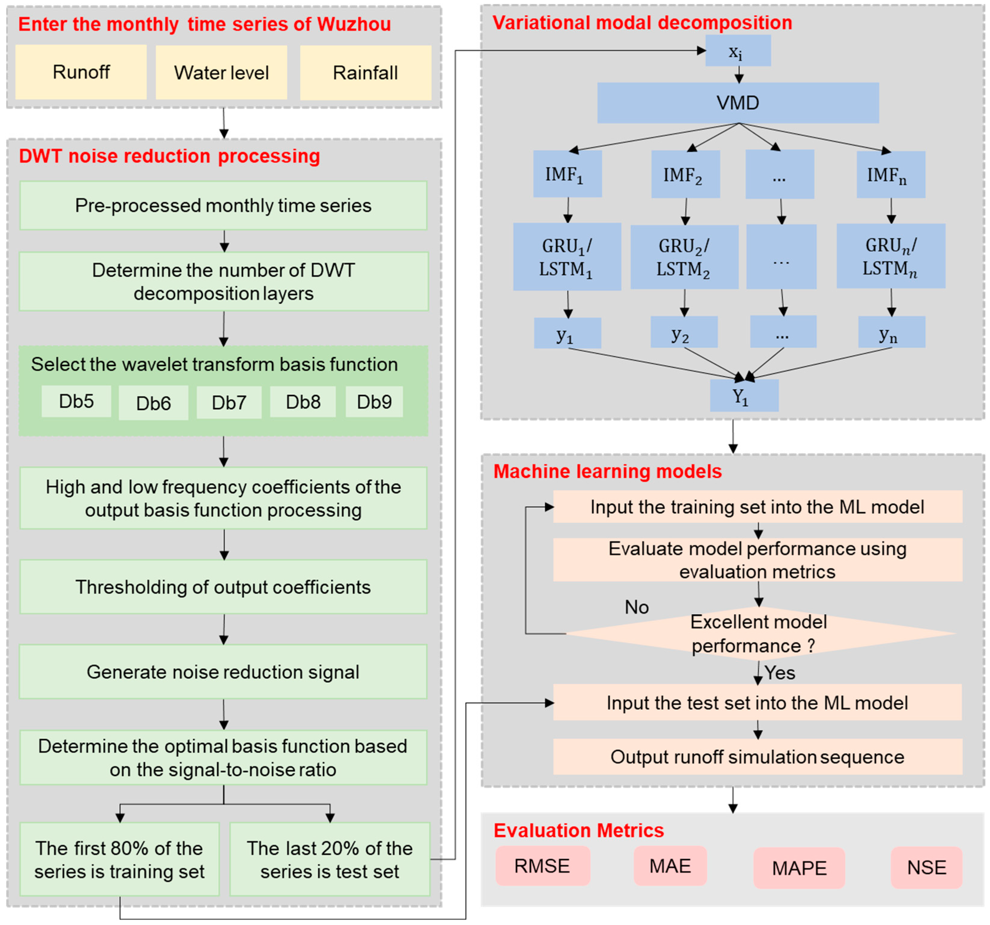
Figure 2 illustrates the research framework via a comprehensive flowchart, delineating the essential procedural stages as follows: (1) Preprocess the measured time series of the monthly runoff (Q), water level (L), and rainfall (P). (2) Denoise the original sequences using the discrete wavelet transform (DWT). (3) Decompose the above sequences into intrinsic mode functions (IMFs) using variational modal decomposition (VMD). (4) Train five models, including GRU, LSTM, DWT–GRU, DWT–LSTM, and DWT–VMD–GRU, incorporating four input combinations: antecedent Q, Q&L, Q&P, and Q&L&P, considering each subsequence (i.e., IMF₁–IMF₅). (5) Test five models and evaluate their performance, particularly the DWT–VMD–GRU model.

3.1. Discrete Wavelet Transform

Two types of wavelet transforms exist: DWT and the continuous wavelet transform. The rainfall and runoff time series inherently exhibit non-stationarity and disruptive noise. To derive meaningful insights for runoff simulation, it is imperative to subject the original series to noise reduction processing. Given the discrete nature of hydrological time series, the former is typically preferred [20]. The formulation of the DWT equation [21,22] is as follows:

$$f_{\left(g,h\right)}=\sqrt{\frac{1}{{a_0}^g}}{\sum }_{t=0}^{n-1}S\left(t\right){\phi }^{*}\left(2^{-g}t-h\right)$$

(1)

where a₀ represents the scale parameter, typically to 2; g and h are integers that determine the wavelet scaling and translation amplitudes, respectively; S(t) signifies the original series at the t-th time step; n denotes sequence length; f_(g,h) is the DWT coefficient; φ is the wavelet function; and ∗ represents the conjugate.

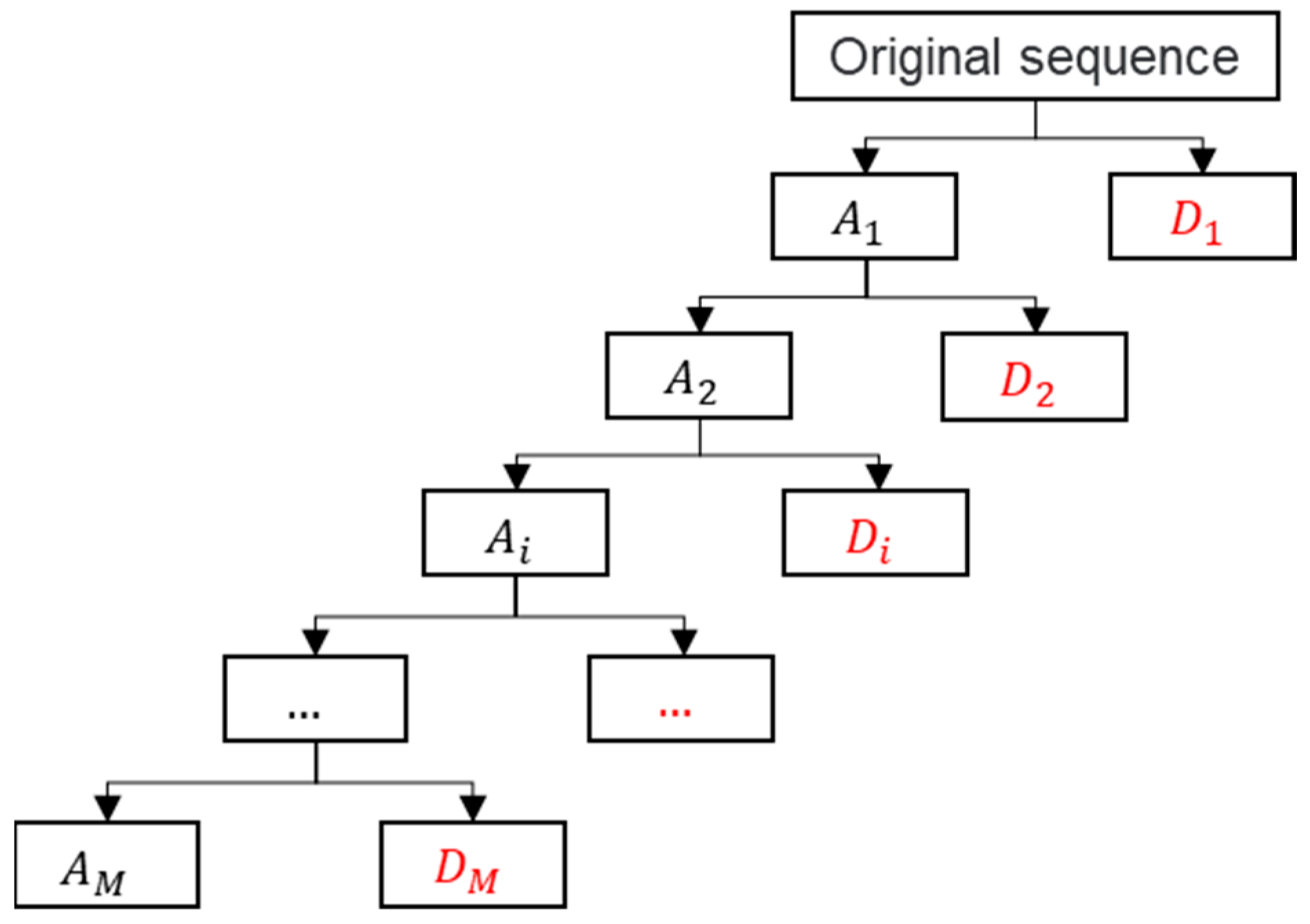
The initial sequence (i.e., noise signal) undergoes decomposition into the approximate and detail signals (Figure 3). Continuous decomposition effectively unveils concealed noisy signals present within the original sequence. While the DWT theoretically accommodates an infinite number of layers, this approach escalates computational complexity significantly. However, the number of DWT layers minimally impacts model prediction [23].

The empirical formula [24] guides the determination of the optimal number of layers:

$$M=\mathrm{int}\left({\log }_{10}n\right)$$

(2)

where M is the number of layers and int denotes the rounding function.

Noise reduction for detail signals is achieved through threshold processing on the decomposition coefficients. A decomposition coefficient (f_(g,h)) that falls below λ_i (a threshold value for the i-th decomposition layer) indicates its predominantly noise-induced nature, warranting its removal. Conversely, coefficients surpassing this threshold suggest proximity to the original signal and thus are retained.

The selection of the wavelet threshold directly influences denoising outcomes, with excessively high values inducing signal distortion and overly low values allowing noise persistence. Notably, λ_i diminishes as the number of decomposition layers increases, as proximity to the original signal heightens. The threshold determination adheres to the expression:

$${\lambda }_i=\frac{\sigma \sqrt{2\ln N_i}}{{\left(\sqrt{2}\right)}^{i-1}}$$

(3)

where i is the decomposition scale, and N_i is the signal length of the i-th layer.

The standard variance of noise (σ) is quantified as:

$$\sigma =\frac{\mathrm{Median}\left(\left|D_1\right|\right)}{0.6745}$$

(4)

where D₁ denotes the detail signal subsequent to the initial wavelet transform and 0.6745 serves as the adjustment factor.

The effectiveness of noise reduction is significantly influenced by the choice of wavelet basis function and the number of wavelet layers employed. The optimal selection of these factors facilitates an enhanced representation of noise within the detail coefficients, thereby simplifying its removal and leading to superior noise reduction outcomes. To quantitatively assess noise reduction performance, the signal-to-noise ratio (SNR) is employed. A larger SNR value corresponds to a more pronounced noise reduction effect. The calculation of SNR follows the formula:

$$\mathrm{SNR}=10\lg \left(\frac{P_1}{P_2}\right)$$

(5)

where P₁ and P₂ signify the effective powers of the original and noise signals, respectively. It is crucial to emphasize that the noise signal represents the disparity between the original and reconstructed signals.

The thresholds for DWT on the monthly runoff, water level, and rainfall sequences were computed to effectively implement this approach. Employing the wavelet toolbox, the hard thresholding method was selected to process the signals, culminating in the derivation of denoised signals.

3.2. Variational Modal Decomposition

VMD is an effective approach tailored to address nonlinear and nonstationary time series; it proficiently resolves the mode mixing problem encountered in EMD through the assignment of the total number (K) of Intrinsic Mode Functions (IMFs), which are subsequently iteratively computed. The k-th IMF is characterized within VMD as a modulation function (u_k) defined by the following expression [25]:

$$u_k\left(t\right)=A_k\left(t\right)\cos \left[{\Phi }_k\left(t\right)\right]$$

(6)

where t is the time step of IMF_k, month. A_k(t) is the upper envelope of the signal. Φ_k(t) is a non-decreasing function.

The number (K) of IMFs is commonly determined by the center frequency method. The optimal value of K is ascertained when the center frequencies of the modal components in the K-th layer and (K + 1)-th layers exhibit similarity. The fundamental principle of VMD revolves around the formulation and solution of variational problems, comprising two distinct steps. In the initial step, a variational problem is constructed. The spectrum (F_k) of the k-th IMF (IMF_k) is expressed as follows:

$$F_k=\left[\delta \left(t\right)+\frac{j}{\pi t}\right]u_k\left(t\right)$$

(7)

where δ(t) represents the Dirac distribution and j is the complex symbol (i.e., j² = −1). Subsequently, the variational problem is solved through the equation:

$$\begin{array}{c}L\left(\left\{u_k\right\},\left\{{\omega }_k\right\},\lambda \right)=\alpha {\displaystyle \sum _{k=1}^K}\Vert {\partial }_t\left\{F_k\right\}{e}^{-j{\omega }_{k}t}{\Vert }_2^2+\Vert f\left(t\right)-{\displaystyle \sum _{k=1}^K}{u}_k\left(t\right){\Vert }_2^2\\ +\langle \lambda \left(t\right),f\left(t\right)-{\displaystyle \sum _{k=1}^K}{u}_k\left(t\right)\rangle \end{array}$$

(8)

where L signifies the augmented Lagrangian function, ω_k denotes the center frequency, (Hz), λ is the Lagrangian multiplier, α represents the penalty factor; and f(t) stands for the original signal. The symbol < > represents the scalar product [26]. The iterative process entails the updating of u_k, ω_k, and λ. Upon completion of the iteration, the decomposed subsequences and ω_k are obtained.

3.3. Recurrent Neural Network

3.3.1. Gated Recurrent Unit

GRU stands as a variant of RNN distinguished by its straightforward architecture, characterized by reset and update gates (Figure 4a) [27]. The reset gate governs the extent to which newly input information aligns with preceding memory. Notably, a gating signal approaching 0 denotes a diminished correlation. Conversely, the gating signal inherent in the update gates influences the extent of past information retention. Ranging between 0 and 1, a value near 0 signifies heightened information loss, while a value closer to 1 signifies preservation [19]. The training of the GRU model was accomplished using the ‘grulayer’ function within MATLAB 2021a.

The reset gate (r_t), update gate (z_t), candidate hidden status ($h_t^{\prime }$), and ultimate hidden status (h_t) are calculated as follows [28]:

$$r_t=\sigma \left(W^{\left(r\right)}{x}_t+U^{\left(r\right)}{h}_{t-1}\right)$$

(9)

$$z_t=\sigma \left(W^{\left(z\right)}{x}_t+U^{\left(z\right)}{h}_{t-1}\right)$$

(10)

$$h_t^{\prime }=\tanh \left(W{x}_t+r_t\odot U{h}_{t-1}\right)$$

(11)

$$h_t=z_t\odot h_{t-1}+\left(1-z_t\right)\odot h_t^{\prime }$$

(12)

where σ represents the logical sigmoid function, compressing activation outcomes within [0, 1], with proximity to 0 indicating information discard; x_t represents the input sequence at time t (current moment); h_t−1 denotes the hidden status information at the moment t − 1; tanh denotes the hyperbolic tangent activation function; ⊙ symbolizes the Hadamard product operator; and W^(r), U^(r), W^(z), U^(z), W, and U correspond to the weight parameters to be learned.

3.3.2. Long Short-Term Memory

LSTM, a derivative of RNNs equipped with LSTM blocks [29], presents a more intricate architecture compared to GRU (Figure 4b). LSTM has exhibited superior performance over alternative RNNs across a diverse array of applications, including time series prediction [30]. The ‘lstmlayer’ function in MATLAB was used to train the LSTM models.

LSTM transmits the hidden state from the previous moment to the current moment, thereby enabling the learning of both short and long-term dependencies. In the LSTM architecture, every cell comprises three layers: the input layer, the recurrent layer, and the output layer. The output layer interfaces with the cell’s three gates: the input gate (i_t, regulating the influx of information from both the prior instant and the current input into the network structure), the forget gate (f_t, determining the extent of memory erasure from the preceding instant), and the output gate (o_t, governing the extent of information emission at the current instant).

$$i_t=\sigma \left(W_i·h_{t-1}+W_i·x_t+b_i\right)$$

(13)

$$f_t=\sigma \left(W_f·h_{t-1}+W_f·x_t+b_f\right)$$

(14)

$$o_t=\sigma \left(W_o·h_{t-1}+W_o·x_t+b_o\right)$$

(15)

$${\tilde{c}}_t=\tanh \left(W_c·h_{t-1}+W_c·x_t+b_c\right)$$

(16)

$$c_t=f_t\odot c_{t-1}+i_t\odot {\tilde{c}}_t$$

(17)

$$h_t=o_t\odot \tanh \left(c_t\right)$$

(18)

where i_t, f_t, and o_t are the input gate, forget gate, and output gate at time t, respectively; σ is the logical sigmoid function to compress the activation result in [0,1]; W_i, W_f, W_o, and W_c are the weight matrix; b_i, b_f, b_o, and b_c are the bias, which is used to control the activation of neurons’ states; ${\tilde{c}}_t$ is a potential vector of the cell state; c_t is the cell state; ⊙ is the Hadamard product operator; and h_t is the hidden status.

3.4. Model Development

The hydrological time series were subjected to DWT and VMD techniques to derive reconstructed sequences encompassing runoff, water level, and rainfall data. Subsequently, a GRU model was trained for simulating runoff patterns, denoted as DWT–VMD–GRU. To ascertain the optimal configuration for the GRU model, initial experimentation was conducted within a range of hidden units spanning from 10 to 30. Through systematic trial and error, the most suitable number of hidden units was identified as 28. Additionally, an exploration of sliding window parameters [31] was undertaken, considering an initial range of 1 to 10 time steps (i.e., 1 month to 10 months). For the DWT–VMD–GRU (Q&P) model, the input variables are runoff and rainfall, so the number of features n = 2; the runoff is simulated along the time series with a sliding window of 1 month, so the sliding window size (lead time) ω = 1; and the time series length is 155 and the sliding step m is set to 1, so the dataset generated after sliding 155 steps is [155,2,1].

3.5. Evaluation Metrics

To assess the effectiveness of the models, we employed a comprehensive set of indices, including the root mean square error (RMSE), mean absolute error (MAE), mean absolute percentage error (MAPE) [32], Nash–Sutcliffe Efficiency (NSE), and Kling–Gupta Efficiency (KGE) [33]. RMSE, MAE, and MAPE exhibit values within the range of (0, +∞), with proximity to 0 indicative of enhanced performance. NSE and KGE range from −∞ to 1, with higher values denoting a better agreement between the observed and predicted data (e.g., a value of 1 signifies a perfect prediction). The simulation effect of the model can be considered as satisfactory when the NSE exceeds 0.5 [34,35]. KGE provides a more comprehensive and balanced assessment by incorporating correlation, bias, and variability, whereas NSE primarily focuses on the proportion of variance [36].

4. Results and Discussion

4.1. Performance of Discrete Wavelet Transform

The application of DWT served to diminish the noise inherent within the monthly runoff, water level, and rainfall time series. Initially, the optimal decomposition layer was determined, leading to the establishment of a two-layer decomposition. Subsequently, Daubechies 5–9 were used as wavelet basis functions (WBFs) and the resulting SNR values after decomposition were computed.

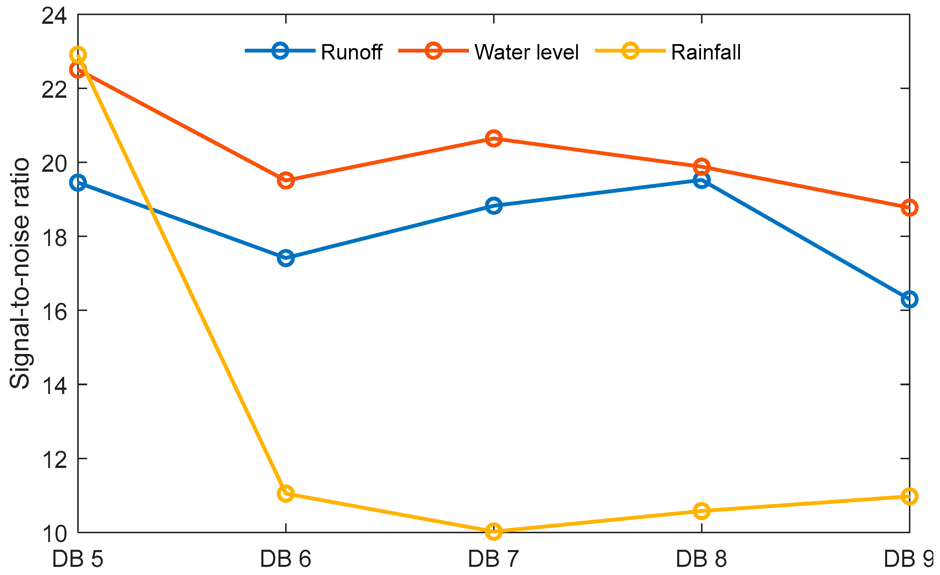
Figure 5 shows the SNR values after decomposition with different WBFs, indicating that Daubechies 5 emerged as the selected WBF for the decomposition of the monthly runoff, water level, and rainfall sequences. This selection was underpinned by the observation that the SNR values for both Daubechies 5 and Daubechies 8 amounted to 19.45 and 19.52, respectively, constituting the highest and second largest values. Furthermore, concerning the water level and rainfall time series, the employment of the Daubechies 5 wavelet consistently yielded the highest SNR values, indicating its efficacy in denoising. With the runoff sequence as the object of simulation, and in situations where SNR values are closely similar (19.45 and 19.52), the preference was for the wavelet with the slightly smaller SNR value, Daubechies 5, to preserve more informative content from the original sequence. This finding aligns with the research conducted by Song et al. (2021) [37], which also employed the WBF set to db5.

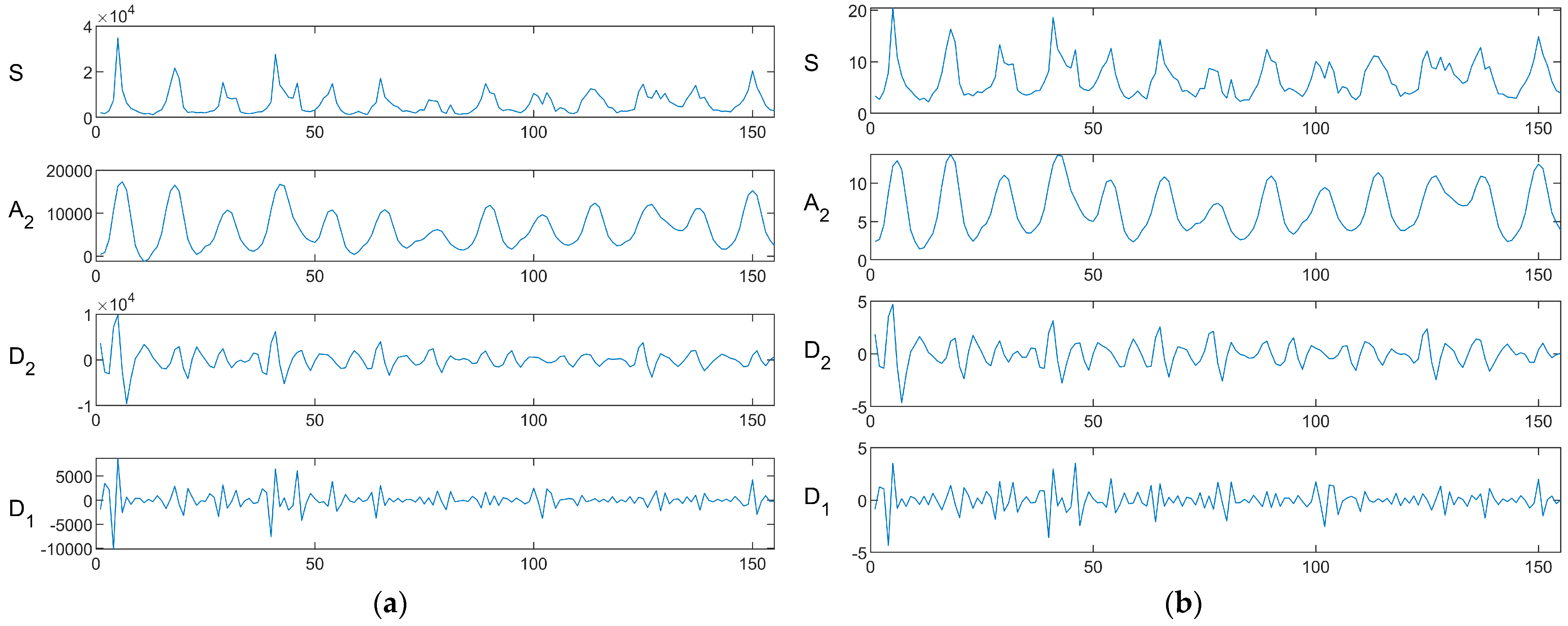
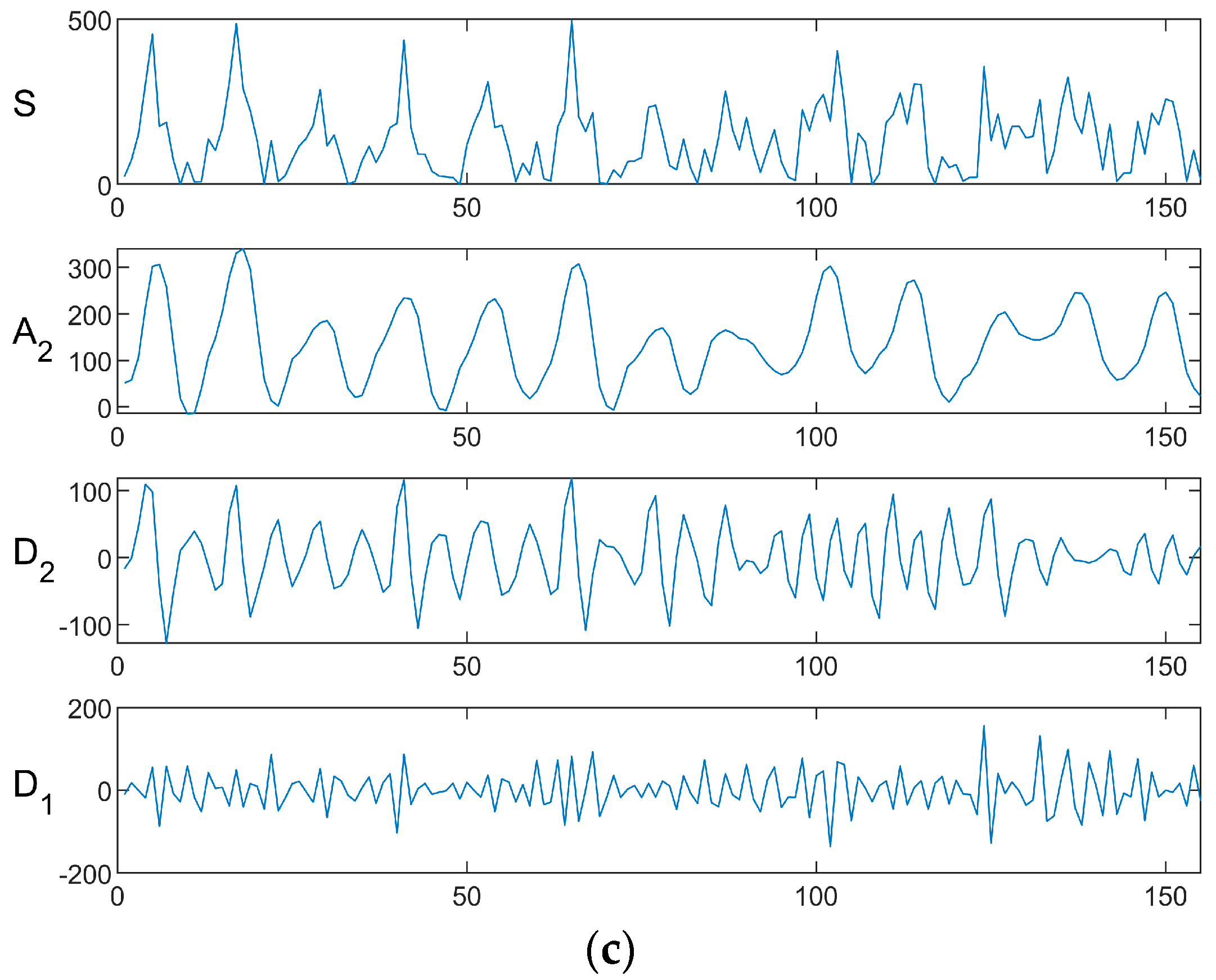
Within this framework, the original monthly runoff, water level, and rainfall sequences underwent decomposition via DWT, generating both approximate components and detail components (Figure 6). Notably, the signals attributed to D₁ exhibited considerable noise, whereas those associated with D₂ displayed comparatively reduced noise. Accordingly, we chose to further denoise the D₁ signals.

4.2. Performance of Variational Modal Decomposition

Table 1. Center frequencies of modal components in different variational modal decomposition scenarios.

Number of IMFs (K) 1	Center Frequency
	IMF1	IMF2	IMF3	IMF4	IMF5	IMF6	IMF7	IMF8
1	0.0261	n/a	n/a	n/a	n/a	n/a	n/a	n/a
2	0.0120	0.2794	n/a	n/a	n/a	n/a	n/a	n/a
3	0.0043	0.3565	0.1297	n/a	n/a	n/a	n/a	n/a
4	0.0038	0.2324	0.1142	0.4163	n/a	n/a	n/a	n/a
5	0.0035	0.2426	0.1149	0.4197	0.1376	n/a	n/a	n/a
6	0.0035	0.2237	0.1143	0.4252	0.1389	0.3253	n/a	n/a
7	0.0034	0.2241	0.1144	0.4252	0.1379	0.3324	0.0577	n/a
8	0.0034	0.2224	0.1144	0.4186	0.1363	0.3352	0.0448	0.4617

Note: ¹ IMFs denote intrinsic mode functions.

presents the outcomes of VMD applied to sequences reconstructed by DWT noise reduction. Notably, among all adjacent modal components, the central frequencies of IMF2 and IMF3 are the closest. As K increases from 6 to 8, the central frequencies of these two modal components converge. This trend suggests that starting from K = 6, the occurrence of modal overlap may become apparent. Conversely, if K is too small, insufficient decomposition may result [38]. Consequently, K = 5 is determined as the optimal count of decomposition layers for VMD.

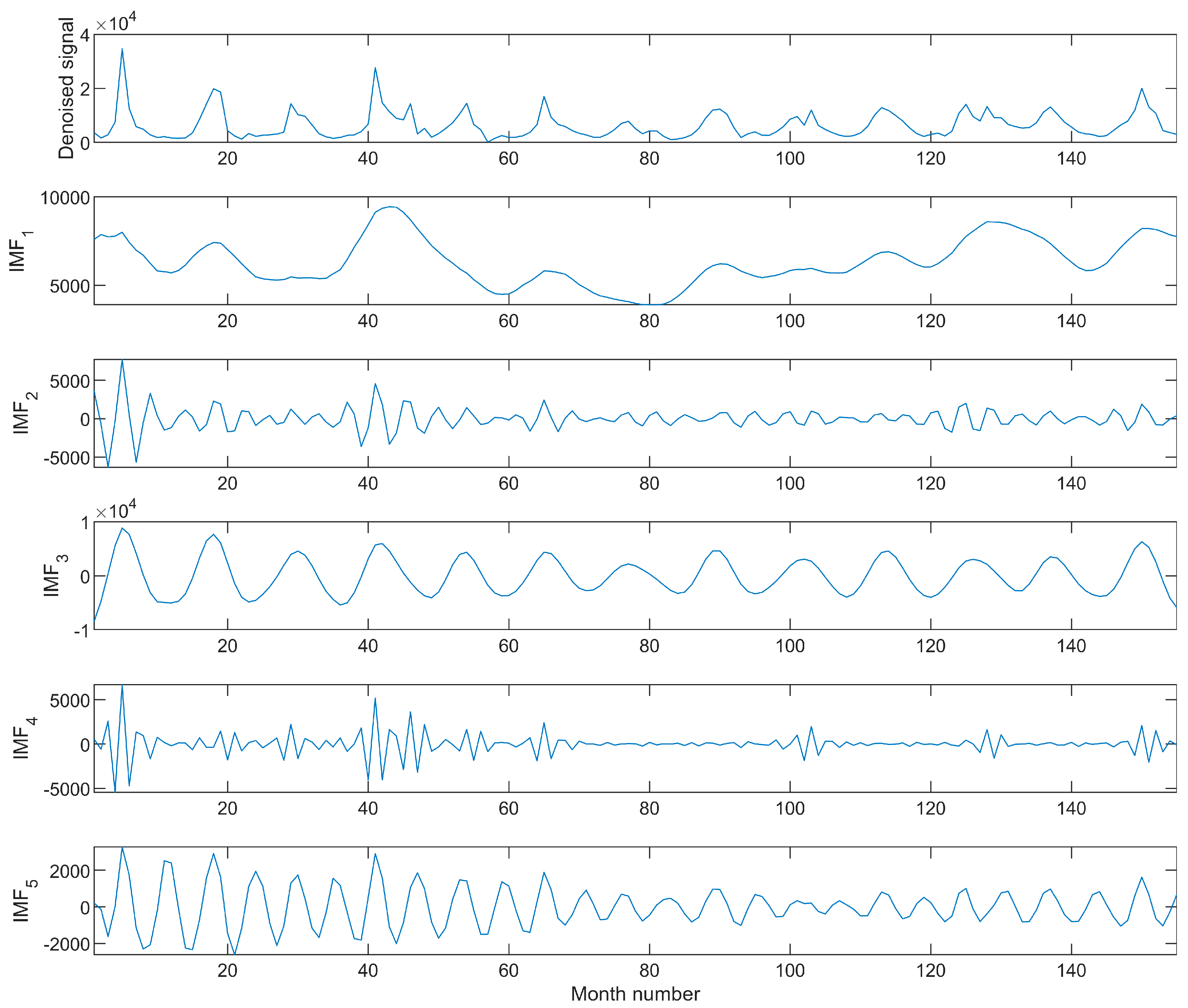
Figure 7 shows the VMD outcomes for the monthly runoff sequence, with K = 5. Evidently, VMD successfully decomposes the monthly runoff sequence into five IMFs, characterized by discernible periodic oscillations. Furthermore, each IMF demonstrates a progressive attenuation in oscillation amplitude as time elapses.

4.3. Performance of Neural Network Models

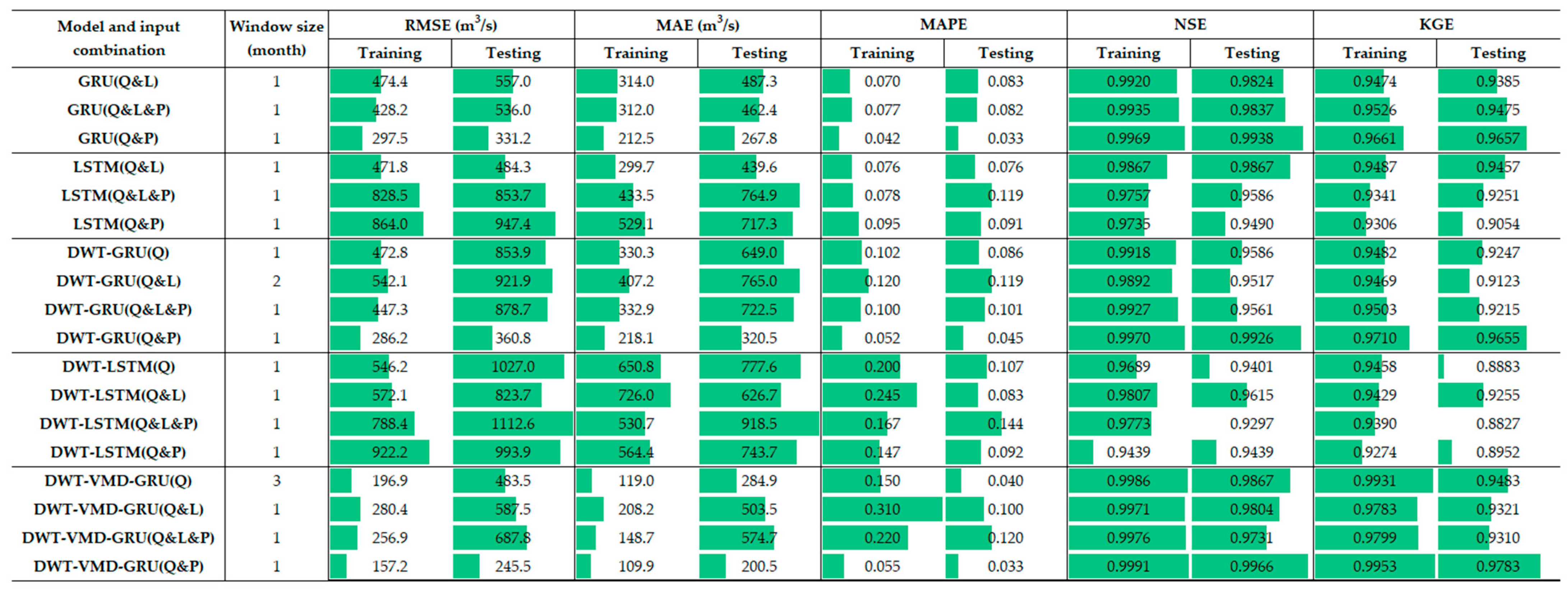
Figure 8 presents an overview of the errors observed across the GRU, LSTM, DWT–GRU, DWT–LSTM, and DWT–VMD–GRU models. Particularly noteworthy is the superior performance exhibited by the DWT–VMD–GRU model across both the training and testing phases. The main findings can be summarized as follows: (1) The DWT–VMD–GRU model, utilizing runoff and rainfall as inputs, exhibits superior generalization ability, consistently outperforming other models across diverse performance metrics. This underscores the effectiveness of the integrated denoising, decomposition, and neural network methodology. (2) Overall, GRU demonstrates superior performance compared to LSTM. However, the mere integration of DWT with the GRU or LSTM models may yield adverse effects. Incorporating VMD alongside DWT substantially improves the simulation efficacy of GRU models.

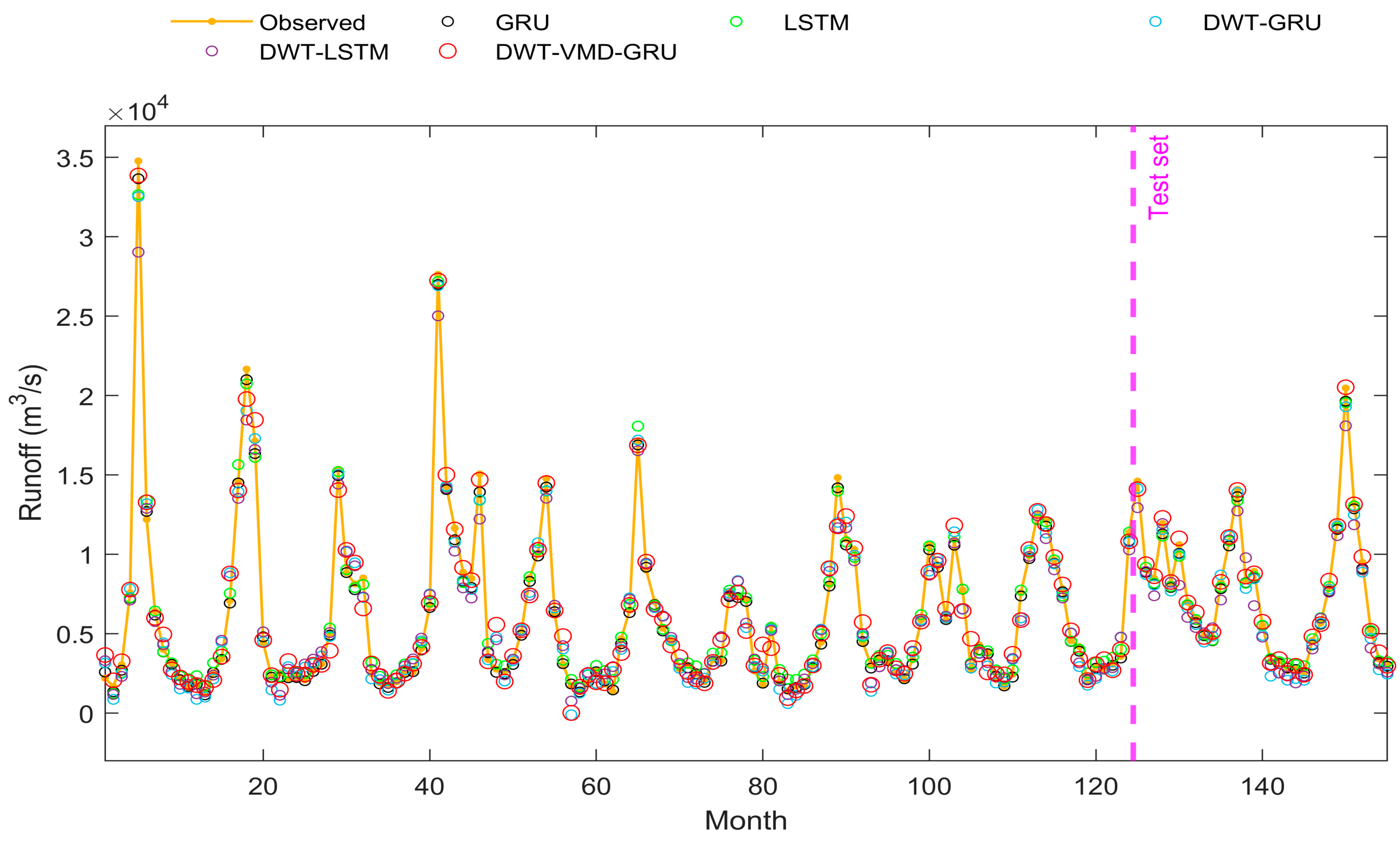
Figure 9 presents the outcomes of GRU(Q&P), LSTM(Q&P), DWT–GRU(Q&P), DWT–LSTM(Q&P), and DWT–VMD–GRU(Q&P). Analysis of the results during the testing phase highlights that DWT–VMD–GRU exhibits the most favorable simulation effect, followed by GRU, DWT–GRU, and DWT–LSTM, with LSTM displaying the least desirable effect. Hence, the following conclusions can be drawn: (1) GRU surpasses the LSTM model in simulation performance. (2) The composite model, integrating denoising, decomposition, and neural network components, exhibits superior simulation performance compared to individual models.

4.4. Window Size and Input Combinations of DWT–VMD–GRU

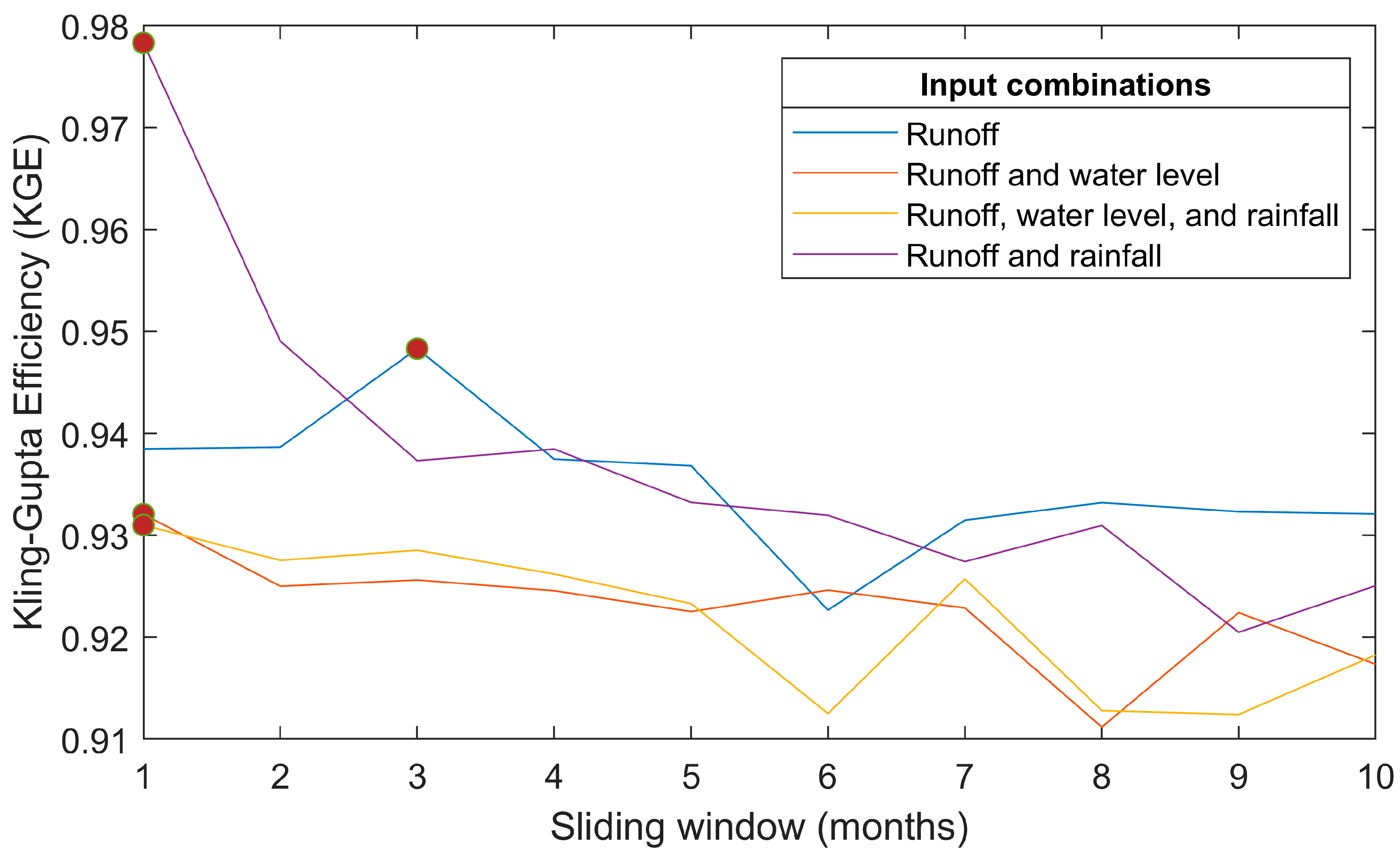
Figure 10 illustrates the KGE values of runoff prediction across various input combinations and sliding window settings. The following was observed: (1) The preferred sliding window duration for diverse combinations of input variables predominantly ranged from 1 to 3. Among the four model input combinations, a decreasing trend in KGE values was evident as the sliding window increased. It suggests that as the sliding window increases, the model performance deteriorates. This observation aligns with the findings of a study conducted by Weng et al. (2023) [39]. (2) All input combinations demonstrated good performance at each sliding window configuration, consistently achieving a KGE exceeding 0.91. Notably, the DWT–VMD–GRU (runoff and rainfall as inputs) model exhibited the highest performance when utilizing a one-month sliding window. This outcome can be attributed to the causal relationship between rainfall and runoff, rooted in physical processes, whereas the association between water level and runoff possesses quasi-linear characteristics. This finding aligns with the research by Zhang et al. (2021) [40], which emphasizes the substantial influence of input variables on the accuracy of runoff prediction using the RNN model.

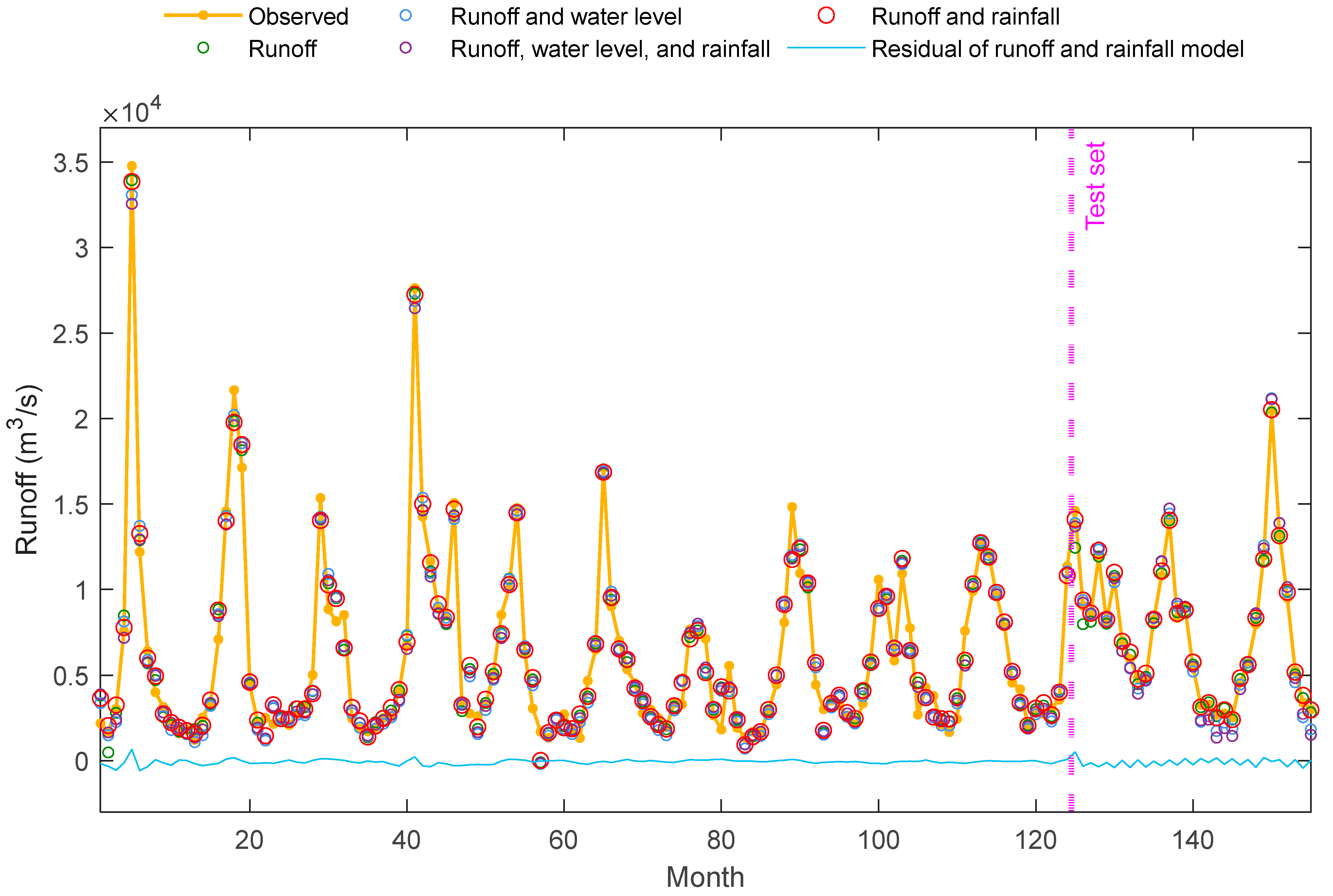
Figure 11 depicts the runoff time series simulated by the DWT–VMD–GRU model utilizing various input variables. Our analysis yields the following conclusions: (1) The examination of the residual plot indicates that the DWT–VMD–GRU model, utilizing runoff and rainfall as inputs, exhibits superior performance compared to three other input combinations, a finding consistent with Tiwari et al.’s (2022) conclusion [41]. (2) Regarding the performance in predicting the maximum annual runoff, the DWT–VMD–GRU model demonstrates that the combination of runoff and rainfall as inputs yields the best results, followed by runoff and water level, and finally, runoff alone. In summary, the model utilizing runoff and rainfall as inputs outperforms the model using only runoff as input in simulating the overall sequence.

Figure 12a depicts flow duration curves (FDCs) for various neural networks, which closely match the observed data, indicating robust performance across training and testing phases. The FDCs perform well in high-flows and less so in low-flows. In the testing phase, the DWT–VMD–GRU(Q&P) model outperforms others in low-flows, followed by the GRU(Q&P) model. Figure 12b shows the FDCs for DWT–VMD–GRU models with different input combinations, with all curves closely matching the observed series, suggesting strong overall model performance. The FDCs of the testing phase perform well in high-flow, capturing extreme flow events. The DWT–VMD–GRU (Q&P) and DWT–VMD–GRU (Q) models excel in high-flows and low-flows, respectively.

5. Conclusions

This study presents a DWT–VMD–GRU model for predicting monthly runoff and evaluates its predictive performance against alternative models. The following conclusions can be drawn: (1) The DWT–VMD–GRU model, utilizing runoff and rainfall time series as inputs, demonstrates superior generalization compared to other models including GRU, LSTM, DWT–GRU, and DWT–LSTM, consistently exhibiting better performance across various evaluation metrics. This superiority is attributed to the denoising effect of DWT, the enhanced sequential feature extraction by VMD, and the enhanced analytical capability of GRU towards the input data. (2) Optimal sliding window durations for different input combinations typically range from 1 to 3 months, with the DWT–VMD–GRU model (using runoff and rainfall) showing peak performance with a one-month sliding window.

Despite the limitations of the dataset, which was constrained by the availability of measured runoff data, this study provides a foundation for future research directions: (1) Evaluate the robustness of the DWT–VMD–GRU model across diverse hydrological stations and its capability to forecast daily and hourly runoff. (2) Evaluate the computational time and learning efficiency of neural networks, employing regularization to reduce the risk of model overfitting, and utilize GPU acceleration technology. (3) Analyze parameter sensitivity, including the hyperparameter optimization of DWT, VMD, and neural networks, as well as conduct principal component analysis [40] to determine a more rational combination of input variables. (4) Explore the integration of other signal decomposition methods, deep learning models, and probabilistic forecasting techniques.

References

1. Xie, K.; Liu, P.; Zhang, J.; Han, D.; Wang, G.; Shen, C. Physics-guided deep learning for rainfall-runoff modeling by considering extreme events and monotonic relationships. J. Hydrol. 2021, 603, 127043. [Google Scholar] [CrossRef]
2. Guo, Y.; Yu, X.; Xu, Y.P.; Chen, H.; Gu, H.; Xie, J. AI-based techniques for multi-step streamflow forecasts: Application for multi-objective reservoir operation optimization and performance assessment. Hydrol. Earth Syst. Sci. 2021, 25, 5951–5979. [Google Scholar] [CrossRef]
3. Yin, H.L.; Guo, Z.L.; Zhang, X.W.; Chen, J.J.; Zhang, Y.N. RR-Former: Rainfall-runoff modeling based on Transformer. J. Hydrol. 2022, 609, 127781. [Google Scholar] [CrossRef]
4. Yin, H.L.; Wang, F.D.; Zhang, X.W.; Zhang, Y.N.; Chen, J.J.; Xia, R.L.; Jin, J. Rainfall-runoff modeling using long short-term memory based step-sequence framework. J. Hydrol. 2022, 610, 127901. [Google Scholar] [CrossRef]
5. Xu, W.X.; Chen, J.; Zhang, X.C.J.; Xiong, L.H.; Chen, H. A framework of integrating heterogeneous data sources for monthly streamflow prediction using a state-of-the-art deep learning model. J. Hydrol. 2022, 614, 128599. [Google Scholar] [CrossRef]
6. Khatun, A.; Sahoo, B.; Chatterjee, C. Two novel error-updating model frameworks for short-to-medium range streamflow forecasting using bias-corrected rainfall inputs: Development and comparative assessment. J. Hydrol. 2023, 618, 129199. [Google Scholar] [CrossRef]
7. Wang, W.C.; Cheng, Q.; Chau, K.W.; Hu, H.; Zang, H.F.; Xu, D.M. An enhanced monthly runoff time series prediction using extreme learning machine optimized by salp swarm algorithm based on time varying filtering based empirical mode decomposition. J. Hydrol. 2023, 620, 129460. [Google Scholar] [CrossRef]
8. Zhao, X.H.; Lv, H.F.; Lv, S.J.; Sang, Y.T.; Wei, Y.Z.; Zhu, X.P. Enhancing robustness of monthly streamflow forecasting model using gated recurrent unit based on improved grey wolf optimizer. J. Hydrol. 2021, 601, 126607. [Google Scholar] [CrossRef]
9. Li, B.J.; Yang, J.X.; Luo, Q.Y.; Wang, W.C.; Zhang, T.H.; Zhong, L.; Sun, G.-L. A Hybrid Model of Ensemble Empirical Mode Decomposition and Sparrow Search Algorithm-Based Long Short-Term Memory Neural Networks for Monthly Runoff Forecasting. Front. Environ. Sci. 2022, 10, 909682. [Google Scholar] [CrossRef]
10. Zuo, G.G.; Luo, J.G.; Wang, N.; Lian, Y.N.; He, X.X. Decomposition ensemble model based on variational mode decomposition and long short-term memory for streamflow forecasting. J. Hydrol. 2020, 585, 124776. [Google Scholar] [CrossRef]
11. He, M.; Wu, S.F.; Kang, C.X.; Xu, X.; Liu, X.F.; Tang, M.; Huang, B.B. Can sampling techniques improve the performance of decomposition-based hydrological prediction models? Exploration of some comparative experiments. Appl. Water Sci. 2022, 12, 175. [Google Scholar] [CrossRef]
12. Zhang, X.; Duan, B.; He, S.; Wu, X.; Zhao, D. A new precipitation forecast method based on CEEMD-WTD-GRU. Water Supply 2022, 22, 4120–4132. [Google Scholar] [CrossRef]
13. Wang, X.; Zhang, S.; Qiao, H.; Liu, L.; Tian, F. Mid-long term forecasting of reservoir inflow using the coupling of time-varying filter-based empirical mode decomposition and gated recurrent unit. Environ. Sci. Pollut. R. 2022, 29, 87200–87217. [Google Scholar] [CrossRef] [PubMed]
14. Xie, T.; Zhang, G.; Hou, J.; Xie, J.; Lv, M.; Liu, F. Hybrid forecasting model for non-stationary daily runoff series: A case study in the Han River Basin, China. J. Hydrol. 2019, 577, 123915. [Google Scholar] [CrossRef]
15. Sibtain, M.; Li, X.; Azam, M.I.; Bashir, H. Applicability of a Three-Stage Hybrid Model by Employing a Two-Stage Signal Decomposition Approach and a Deep Learning Methodology for Runoff Forecasting at Swat River Catchment, Pakistan. Pol. J. Environ. Stud. 2021, 30, 369–384. [Google Scholar] [CrossRef]
16. Liu, B.C.; Chen, J.L.; Guo, X.L.; Wang, Q.S. Study on NO2 concentration prediction in Tianjin based on DWT-GRU model. Environ. Sci. Technol. 2020, 43, 94–100. [Google Scholar]
17. Xu, Z.; Zhou, J.; Mo, L.; Jia, B.; Yang, Y.; Fang, W.; Qin, Z. A Novel Runoff Forecasting Model Based on the Decomposition-Integration-Prediction Framework. Water 2021, 13, 3390. [Google Scholar] [CrossRef]
18. Dong, J.; Wang, Z.; Wu, J.; Cui, X.; Pei, R. A Novel Runoff Prediction Model Based on Support Vector Machine and Gate Recurrent Unit with Secondary Mode Decomposition. Water Resour. Manag. 2024, 38, 1655–1674. [Google Scholar] [CrossRef]
19. Gao, S.; Huang, Y.F.; Zhang, S.; Han, J.C.; Wang, G.Q.; Zhang, M.X.; Lin, Q.S. Short-term runoff prediction with GRU and LSTM networks without requiring time step optimization during sample generation. J. Hydrol. 2020, 589, 125188. [Google Scholar] [CrossRef]
20. Apaydin, H.; Sibtain, M. A multivariate streamflow forecasting model by integrating improved complete ensemble empirical mode decomposition with additive noise, sample entropy, Gini index and sequence-to-sequence approaches. J. Hydrol. 2021, 603, 126831. [Google Scholar] [CrossRef]
21. Abebe, S.A.; Qin, T.L.; Zhang, X.; Yan, D.H. Wavelet transform-based trend analysis of streamflow and precipitation in Upper Blue Nile River basin. J. Hydrol. Reg. Stud. 2022, 44, 101251. [Google Scholar] [CrossRef]
22. Alizadeh, F.; Gharamaleki, A.F.; Jalilzadeh, M.; Akhoundzadeh, A. Prediction of River Stage-Discharge Process Based on a Conceptual Model Using EEMD-WT-LSSVM Approach. Water Resour. 2020, 47, 41–53. [Google Scholar] [CrossRef]
23. Ba, H.; Hu, T.; Yuan, Y.; Zhang, S.; Liang, Y. Monthly Runoff Forecast of the Three Gorges Reservoir Based on Wavelet Transform and Artificial Neural Network Model. Water Resour. Power 2022, 40, 10–13+49. [Google Scholar]
24. Amininia, K.; Saghebian, S.M. Uncertainty analysis of monthly river flow modeling in consecutive hydrometric stations using integrated data-driven models. J. Hydroinformatics 2021, 23, 897–913. [Google Scholar] [CrossRef]
25. Seo, Y.; Kim, S.; Singh, V.P. Machine Learning Models Coupled with Variational Mode Decomposition: A New Approach for Modeling Daily Rainfall-Runoff. Atmosphere 2018, 9, 251. [Google Scholar] [CrossRef]
26. Kwak, J.; Lee, J.; Jung, J.; Kim, H.S. Case Study: Reconstruction of Runoff Series of Hydrological Stations in the Nakdong River, Korea. Water 2020, 12, 3461. [Google Scholar] [CrossRef]
27. Zou, Y.S.; Wang, J.; Lei, P.; Li, Y. A novel multi-step ahead forecasting model for flood based on time residual LSTM. J. Hydrol. 2023, 620, 129521. [Google Scholar] [CrossRef]
28. Xu, C.; Wang, Y.; Fu, H.; Yang, J. Comprehensive Analysis for Long-Term Hydrological Simulation by Deep Learning Techniques and Remote Sensing. Front. Earth Sci. 2022, 10, 875145. [Google Scholar] [CrossRef]
29. Fan, J.S.; Liu, X.F.; Li, W.D. Daily suspended sediment concentration forecast in the upper reach of Yellow River using a comprehensive integrated deep learning model. J. Hydrol. 2023, 623, 129732. [Google Scholar] [CrossRef]
30. Park, K.; Jung, Y.; Seong, Y.; Lee, S. Development of Deep Learning Models to Improve the Accuracy of Water Levels Time Series Prediction through Multivariate Hydrological Data. Water 2022, 14, 469. [Google Scholar] [CrossRef]
31. Li, G.; Zhu, H.; Jian, H.; Zha, W.; Wang, J.; Shu, Z.; Yao, S.; Han, H. A combined hydrodynamic model and deep learning method to predict water level in ungauged rivers. J. Hydrol. 2023, 625, 130025. [Google Scholar] [CrossRef]
32. Huan, S. A novel Interval Decomposition Correlation Particle Swarm Optimization-Extreme Learning Machine model for short-term and long-term water quality prediction. J. Hydrol. 2023, 625, 130034. [Google Scholar] [CrossRef]
33. Kling, H.; Fuchs, M.; Paulin, M. Runoff conditions in the upper Danube basin under an ensemble of climate change scenarios. J. Hydrol. 2012, 424, 264–277. [Google Scholar] [CrossRef]
34. Moriasi, D.N.; Arnold, J.G.; Van Liew, M.W.; Bingner, R.L.; Harmel, R.D.; Veith, T.L. Model Evaluation Guidelines for Systematic Quantification of Accuracy in Watershed Simulations. Trans. ASABE 2007, 50, 885–900. [Google Scholar] [CrossRef]
35. Moriasi, D.N.; Gitau, M.W.; Pai, N.; Daggupati, P. Hydrologic and Water Quality Models: Performance Measures and Evaluation Criteria. Trans. ASABE 2015, 58, 1763–1785. [Google Scholar]
36. Knoben, W.J.M.; Freer, J.E.; Woods, R.A. Technical note: Inherent benchmark or not? Comparing Nash-Sutcliffe and Kling-Gupta efficiency scores. Hydrol. Earth Syst. Sc. 2019, 23, 4323–4331. [Google Scholar] [CrossRef]
37. Song, C.; Chen, X.H.; Wu, P.; Jin, H.Y. Combining time varying filtering based empirical mode decomposition and machine learning to predict precipitation from nonlinear series. J. Hydrol. 2021, 603, 126914. [Google Scholar] [CrossRef]
38. Luan, C. Jiyu VMD-LSTM de heliu liuliang yuce fangfa [River flow prediction method based on VMD-LSTM]. Water Resour. Hydropower Northeast. China 2024, 42, 23–29. [Google Scholar]
39. Weng, P.; Tian, Y.; Liu, Y.; Zheng, Y. Time-series generative adversarial networks for flood forecasting. J. Hydrol. 2023, 622, 129702. [Google Scholar] [CrossRef]
40. Zhang, J.W.; Chen, X.H.; Khan, A.; Zhang, Y.K.; Kuang, X.X.; Liang, X.Y.; Taccari, M.L.; Nuttall, J. Daily runoff forecasting by deep recursive neural network. J. Hydrol. 2021, 596, 126067. [Google Scholar] [CrossRef]
41. Tiwari, D.K.; Tiwari, H.L.; Nateriya, R. Runoff modeling in Kolar river basin using hybrid approach of wavelet with artificial neural network. J. Water Clim. Change 2022, 13, 963–974. [Google Scholar] [CrossRef]
Figure 1. Study site.
Water 16 01552 g001
Figure 2. Flowchart of monthly runoff simulation based on sequence preprocess techniques and machine learning (ML) models. Discrete wavelet transform, DWT; gate recurrent unit, GRU; long short-term memory, LSTM; mean absolute error, MAE; mean absolute percentage error, MAPE; Nash–Sutcliffe Efficiency, NSE; root mean square error, RMSE; variational modal decomposition, VMD.
Water 16 01552 g002
Figure 3. Diagram of discrete wavelet transform (DWT). Approximate components, Ai; detail components, Di. i and M are the serial number and total number of decomposed layers.
Water 16 01552 g003
Figure 4. Architectures of (a) gated recurrent unit and (b) long short-term memory. σr and σz stand for the logical sigmoid function of the reset gate and the update gate. σf, σi, and σo stand for the logical sigmoid function of the forget, input, and output gates at t-th time step.
Water 16 01552 g004
Figure 5. Signal-to-noise ratio after decomposition with various basis functions. Daubechies, DB.
Water 16 01552 g005
Figure 6. Discrete wavelet transform coefficient of (a) runoff, (b) water level, and (c) rainfall time series. Ai, i-th approximate component; Di, i-th detail component; S, original signal.
Water 16 01552 g006aWater 16 01552 g006b
Figure 7. Decomposition monthly runoff series by variational modal decomposition with K = 5. It includes the denoised sequence and intrinsic mode functions (IMFs).
Water 16 01552 g007
Figure 8. Error and optimal sliding window size of GRU, LSTM, DWT–GRU, DWT–LSTM, and DWT–VMD–GRU models. Discrete wavelet transform, DWT; gate recurrent unit, GRU; Kling–Gupta Efficiency, KGE; long short-term memory, LSTM; mean absolute error, MAE; mean absolute percentage error, MAPE; Nash–Sutcliffe Efficiency, NSE; root mean square error, RMSE; variational modal decomposition, VMD. Note: runoff as inputs, Q; runoff and water level as inputs, Q&L; runoff, water level, and rainfall as inputs, Q&L&P; runoff and rainfall as inputs, Q&P.
Water 16 01552 g008
Figure 9. Observed monthly runoff series and predicted series by neural network models. The input variables for all models encompass monthly runoff and rainfall series. Discrete wavelet transform, DWT; gate recurrent unit, GRU; long short-term memory, LSTM; variational modal decomposition, VMD.
Water 16 01552 g009
Figure 10. Kling–Gupta Efficiency values of DWT–VMD–GRU in predicting monthly runoff with different input combinations and sliding windows. Discrete wavelet transform, DWT; dots illustrate the optimal number of sliding Windows for each input combination; gate recurrent unit, GRU; variational modal decomposition, VMD.
Water 16 01552 g010
Figure 11. Monthly runoff predicted by DWT–VMD–GRU models with different input combinations. Discrete wavelet transform, DWT; gate recurrent unit, GRU; variational modal decomposition, VMD.
Water 16 01552 g011
Figure 12. Flow duration curves: (a) optimal models: GRU, LSTM, DWT–GRU, DWT–LSTM, and DWT–VMD–GRU; (b) DWT–VMD–GRU models with various input combinations. Solid lines indicate flow duration curves across both training and testing phases; dashed lines illustrate flow duration curves specifically for the testing phase. Discrete wavelet transform, DWT; gate recurrent unit, GRU; long short-term memory, LSTM; variational modal decomposition, VMD. Q, L, and P denote runoff, water level, and precipitation time series, respectively.
Water 16 01552 g012