Article

Socio-Spatial Analysis of Water Affordability at Small Scales: A Needs-Based Approach

1
Geography Department, Campus UAB, Autonomous University of Barcelona, Plaça del Coneixement, 08193 Bellaterra, Spain
2
Institut Metròpoli, Plaça del Coneixement, Campus UAB, Autonomous University of Barcelona, 08193 Bellaterra, Spain
3
Catalan Institute for Water Research (ICRA-CERCA), Edifici H2O, Girona University, C/Emili Grahit, 101, 17003 Girona, Spain
4
Geography Department, Campus Barri Vell, Girona University, Edif. St. Domènec ll, Plaça Ferrater i Mora, 1, 17004 Girona, Spain
*
Author to whom correspondence should be addressed.
Water 2024, 16(11), 1496; https://doi.org/10.3390/w16111496
Submission received: 28 April 2024 / Revised: 21 May 2024 / Accepted: 22 May 2024 / Published: 24 May 2024
(This article belongs to the Special Issue Socio-Economics of Water Resources Management)

Abstract

:
Water affordability as a dimension of water poverty is becoming an increasing source of concern in cities of the Global North. Studies on water affordability are either based on water wants and not needs or tend to use spatial scales too large for effective analyses of local inequities that can truly guide policy actions. In this contribution, we calculate and map a Water Affordability Index (WAI) based on the minimum water requirement of 100 litres/person/day at the scale of the census tract for the Metropolitan Area of Barcelona. We also apply global and local spatial autocorrelation analyses to investigate spatial relationships between the WAI and poverty-related sociodemographic variables. Results show that, even though average WAI values are moderate, the distribution pattern of higher and lower values tends to be clustered in some districts and neighbourhoods of the study area. Bivariate correlations indicate that water affordability is not only related to poverty variables but also to the diversity of water prices. Findings exemplify how the constructed index can complement existing affordability indicators, revealing and mapping important risk groups struggling to meet the costs of essential water needs. Water affordability could be mitigated by supportive water pricing policies for vulnerable households in water poverty hotspots.

1. Introduction

1.1. Theoretical Framework

The concept of water poverty achieved international recognition when the United Nations declared access to water and sanitation a human right [1]. Individuals, communities, regions, and countries could be defined as water-poor if they failed to comply with at least one of the five dimensions of the human right to water and sanitation, namely that water must be safe, acceptable, sufficient, physically accessible, and affordable [2,3,4]. Safe, sufficient, and physically accessible water represents a major problem in many developing countries [5]. Although access to water is by no means universally safe and secure in the Global North [6,7], for most water-poor people in rich countries, affordability, or the inability to pay for water, remains the main problem [6,8,9]. This ushers in water security concerns even in affluent societies enjoying extensive network coverage and sophisticated treatment systems [9]. Since our focus is on the Global North, in this paper we have understood water poverty as, primarily but not exclusively, an affordability question [8] and have attempted to estimate water affordability in quantitative terms using as an example the Metropolitan Area of Barcelona (MAB). We have employed a needs-based approach considering only those uses of water satisfying minimum standards of living according to the literature [10,11]. The scale chosen for analysis is relatively rare in Europe where most studies select data at the national, regional or in some cases municipal levels but rarely at submunicipal units such as census tracts (CTs), for which detailed sociodemographic information is increasingly available in many European countries. Through a fine-grained spatial analysis, our study attempts to shed light on the relationship between poverty and water affordability. In disentangling the relationships between water affordability and poverty, we have identified spatial clusters of unaffordability and have tested the relationships of water affordability with variables such as income, gender, migration, or age. All these calculations may be of interest to guide the application of policy actions specifically tailored to the different socio-spatial realities found in urban areas across the Global North. This approach would complement analyses based on household-level surveys collecting information on water affordability (e.g., the European Survey on Income and Living Conditions [EU-SILC]), allowing us to detect where, and in some sense also why, water affordability may be a problematic social issue. Results at the submunicipal scale may assist in the design of site-specific policies for helping households face an issue of growing concern and social impacts.
Given the multifactorial nature of water poverty [12], the main goal of the paper is to build an affordability index based not only on income but also on household data and water prices and taxes. Moreover, and to avoid superfluous uses, we developed an index that includes essential water uses only. The first objective of the paper was to provide a quantitative estimation of household water affordability at the CT level based on this index. The water affordability index is understood as the proportion of the economic cost (in EUR) of water for essential uses as reflected in the water bills over the total household income. Due to the disparity of affordability thresholds and the wide variety of methods and criteria to define a household as water-poor [9,13], we did not seek to establish such a threshold or to make comparisons with other thresholds. Rather, our interest lay in finding possible associations of water affordability with sociodemographic variables used in poverty and deprivation studies at appropriate scales such as gender [14], population at risk of poverty [15], foreign-born population [16] or economic inequality [17]. Along this line, the second and third objectives included, respectively, the identification of spatial clusters of water affordability, and the comparison of affordability with sociodemographic variables used in poverty studies.
The paper is organised as follows. After this introduction, we reviewed the literature on water affordability with an emphasis on the Global North. In this review, we paid attention to the debate on the selection of the appropriate threshold to define water-poor households, particularly on the figure of 3 percent of available household income spent on water which remains the most cited benchmark for defining water-poor households [9]. The following section presents the materials and methods of analysis. As stated above, our study area was the Metropolitan Area of Barcelona (MAB), but our scale of work was the CT for which information on the economic cost of water and household income, as well as other sociodemographic variables, was available. After calculating the water affordability index (WAI) for each CT, spatial autocorrelation analyses were developed to test the robustness of the resulting spatial clusters of water affordability which we then related to several sociodemographic variables. In the results section, we present the main findings on water affordability in the MAB and its internal dynamics. Results were discussed in terms of their possible relation with other studies such as the Survey of Income and Living Conditions conducted in the MAB, and especially, regarding the possible relationships between water affordability and variables traditionally associated with poverty. Finally, in the conclusions, we summarise the most relevant aspects of the research, assess possible limitations of the study, and propose some possible avenues for future research on this topic.

1.2. Water Poverty as an Affordability Problem: An Emerging Field of Study

The literature on water poverty as an affordability problem in the Global North is extensive [11,18]. Many contributions focus on the United States where water poverty has grown worse in recent years as water prices have risen above the capacity to pay for low-income households [6,13,19,20,21]. In Europe, water poverty has been studied in countries such as the UK [22], France [23]; Italy [24], Belgium [10], Portugal [9], Spain [8,25,26,27,28], and the so-called transition countries [29]. Most studies work with household data although the scale of statistical aggregation is usually much larger (city or metropolitan area and more frequently region or country). To our knowledge, water affordability studies using CT data are rare in Europe in contrast with the US where the use of this spatial unit is more common [21].
Most of the contributions aim at finding quantitative thresholds for affordability from which a condition of water poverty can be defined. Usually, the threshold is the quotient, represented by an index or a percentage defined as the Water Affordability Index, between the economic cost of water for households and household income. In Europe, the most common threshold for defining a household in a condition of water poverty is when the economic cost of water represents 3 percent or more of household income [9,13,30]. It is acknowledged that such an economic effort is high enough to force households to refrain from spending money on other basic needs [19]. The figure of 3 percent has become the standard benchmark for international comparability in water poverty studies [30]. However, both the numerator (water expenditure) and denominator (household income) have been criticised for possibly masking large water consumption by rich households (lawns, gardens, and swimming pools) based on wants and not on needs [19]. Perhaps more significantly, when using averaged aggregated data at the regional or national level of household water expenditure and income in Global North countries, the 3 percent threshold appears to be too high to rule out the presence of households under these conditions. Although the WAI in Global North countries is lower because of higher average incomes, the higher cost of living may mask cases of water poverty masked by lower WAIs than those of other countries. According to Smets [30], the average values of the WAI for 14 countries of Western Europe oscillate between 0.6 and 1.8 percent with an average value of 1.1 percent. For Eastern European transition countries, the range is between 1.5 and 4.6 percent with an average value of 2.6 percent or more than twice the figure for Western Europe. Hence, the selection of the threshold appears to be related to the level of development. Thus, and rather convincingly, other authors argue that the 3 percent threshold would be more meaningful for developing rather than developed countries [24].
The identification of the water-poor at the level of households using the 3 percent benchmark is only possible through specific survey work such as Martins [9] for Portugal or Domene [31] for the Metropolitan Area of Barcelona. When aggregated data are used, the most extreme values tend to dissolve among averages. The European Survey on Income and Living Conditions [32] includes data from interviews at the household level that may be extrapolated to national, regional, or provincial scales but not to urban or suburban units. Therefore, for large urban agglomerations, the lack of disaggregated data on water- and energy-poor households, may impede the identification of spatial clusters of water poverty. Cluster identification facilitates the location of vulnerable areas in terms of water affordability.
To make visible water-poor households, more refined methods of estimation can be found in the literature [11,13]. First, for the numerator, it has been proposed that the economic cost of water for households includes only the cost of essential uses (drinking, cooking, personal hygiene). Some authors have produced very precise estimations of the water satisfying these basic needs [10,33], although substantial variations may be found between and within countries. Other authors have estimated essential water uses from the proportion of this water statistically determined to be inelastic and therefore essential [34] while others have opted for using a fixed figure such as the 100 L/person/day (lpd) of the OECD considered to cover basic needs for households in Global North countries [35]. As to the denominator, some approaches use income subgroups, usually defined as those receiving a fraction of average income such as the lowest income quintile in the United States [20] or the 40 and 60 percent of the average income in certain European countries [10,30]. In Western Europe, when considering only the household group with an average income of 40 percent or less than the national average income, the WAI climbs to 2.75 percent [30]. At any rate, values above 3 percent remain rare, making evident the need for other approximations to water poverty beyond this criterion.

2. Materials and Methods

2.1. Case Study: The Metropolitan Area of Barcelona (MAB)

The Metropolitan Area of Barcelona (MAB), one of the most populated conurbations of Southern Europe, is located in the northeast of the Iberian Peninsula, The MAB (636 km2) includes 36 municipalities and more than 3.3 million people, combining highly compact areas with low-density enclaves [8]. Moreover, the MAB concentrates on important poverty hotspots and water prices that are among the highest in Spain [36,37]. Average domestic water consumption in the MAB was around 105 lpd in 2018, with averages at the municipal level varying from 85 to 140 lpd, these differences are mostly explained by urban density and income levels in the different municipalities [31].
The MAB may be an interesting setting for studying the spatial distribution of water affordability, given the presence of strong spatial segregation patterns in terms of income and other variables defining socioeconomic status [38], the diversity in the number of companies providing the water supply services, and the differences in water prices according to water companies and municipalities. In 2018, average household incomes ranged from EUR 27,367/year in the poorest municipality to EUR 61,718/year in the wealthiest (refer to Table A1 in Appendix A); average household size oscillates between 1.9 and 3.44 persons per household while the municipal population density in 2021 ranged from 21,406 inh/km2 to 133 inh/km2.
In 2020, one in four inhabitants of the MAB was at risk of poverty, defined as the population with an income 60 percent or less than the average income of the MAB. This figure had risen by 23 percent in comparison with the figure before the COVID-19 pandemic. Furthermore, 12 percent of the metropolitan population was at risk of extreme poverty, defined as the population with an income 30 percent or less than the average income of the MAB [39]. Data from the Spanish Survey on Income and Living Conditions (EU-SILC) showed that, using the 3 percent benchmark, around 10 percent of MAB households (125,300) were in water poverty in 2019 [40]. If only households at risk of poverty were considered, this figure rose to 83 percent of the total. Water prices also show important variations among the municipalities. For an average consumption of 12 m3/month, in 2022 some residents paid EUR 1.49/m3 while others paid EUR 3.27/m3 [41].
If households are granted the status of “vulnerable” by municipal social services they are eligible for discounts on the water bill [8]. However, it is not possible to introduce subsidies in this study due to the lack of data at an appropriate scale.

2.2. Calculation of the Water Affordability Index at the Census Tract Level

We defined the Water Affordability Index (WAI) as the percentage of household income allocated to the payment of essential water uses. We did not include the total amount of the water bill but only the cost of the water for fulfilling basic needs such as drinking, cooking, personal hygiene and washing. In our case, we selected the standard figure of 100 L/person/day (lpd) proposed by the OECD to cover all these basic needs [35]. As to the other component of the index, we used the average household income of the area estimated at the CT level [34]. The CT scale allowed us to work on a small spatial scale and at the same time comparable with other similar spatial units that contain the same type of information for other European countries such as Belgium (Statistical Sector), France (Statistical Block), or Italy (Census District) [42]. Unfortunately, the structure of Spanish statistical data [32] precluded refining this variable to include only households at risk of poverty (households with an income of 60 percent or less than the average metropolitan income).
In order to calculate the WAI for the 2146 CTs of the MAB, two sets of data were prepared. First and for the year 2018, we obtained sociodemographic and economic data at the CT level (population, number of households, average size of households, and average household income) for the 36 municipalities included in the MAB. The data were provided by the Spanish Statistical Institute [43] together with data concerning the rest of the sociodemographic variables used in the study. The second set of data concerned the cost of the water bill in each municipality. Both sets of data require information at different levels of disaggregation, which is generally available in many European countries. Currently, 23 of the 36 municipalities are supplied by “ABEMCIA”, a public–private company (80 percent of the shares are owned by the private company “Aigües de Barcelona”) while the rest are served by other public–private companies, private companies, or public companies (the latter only 2 out of the 36 municipalities). The amount of the water bill presents differences between municipalities according to the items included (water supply and sanitation, and several taxes). We obtained information on the water price from the “Catalan Observatory Water Prices” [41]. The Catalan Water Agency provides an online tool to calculate the monthly amount of the water bill for each municipality according to different monthly consumptions (from 1 m3 to 30 m3). The amount of the invoice is broken down into different concepts: the water supply rate, the sewerage fee, and the regional water fee. In this case, the total cost included the price of water plus these three components, plus VAT. Moreover, to this basic structure, some municipalities such as Barcelona add an extra item which is the domestic waste fee. Given the complexity of the water bill we provide below a basic formula with all the components included in the bill:
TWBA = WSF + SF + RWT + VAT
where:
  • TWBA is the total amount of the bill (in EUR).
  • WSF is the Water Supply Fee, including the Fixed Consumption Fee, the Variable Consumption Fee, and the Water Meter fee. The Fixed Consumption Fee depends on the number of water-using devices present in homes (taps, baths, toilets, etc.), and, in the case of ABEMCIA (the largest water company in the MAB) ranges from EUR 2.6/month (one tap, one toilet) to EUR 64/month, (households with several bathrooms and a garden and swimming pool). The Variable Consumption Fee includes the cost of the water consumed, which is priced according to a progressive block structure. On average, the fixed fee may represent up to 25 percent of the cost of the water supplied to households and a smaller proportion depending on the amount of the different taxes collected.
  • SF is the Sewerage Fee.
  • RWT is the Regional Water Tax. This tax also varies according to consumption blocks.
  • VAT, which is generally 10% of the total bill except for the water meter fee, which is 21%.
For the purposes of this paper, we calculated the average water consumption of households based on the 100 lpd benchmark, multiplying the amount consumed by the average household size of each CT. We are aware that this method may overestimate water consumption and expenditure in the household regarding essential needs due to economies of scale, such as the use of washing machines. However, by excluding non-essential uses, we were able to gain a more realistic perspective on households with affordability issues. Subsequently, figures in litres/household/day were converted into cubic metres per household per month, with final quantities oscillating between 7 and 9 cubic metres. This total water consumption per household was then multiplied by theoretical costs in the water bill of each municipality, considering that these costs included the fixed components, the variable components, and the different taxes in each municipality and we obtained the total water bill amount (TWBA). Once the TWBA was obtained for each CT, it was divided by the average net income of each household (AHI) in that same CT and multiplied by 100 to obtain the percentage (WAI).
W A I = T W B A H I × 100
where:
  • WAI is the Water Affordability Index (in %).
  • TWBA is the total amount of the bill (in EUR).
  • AHI is the Average Household Income (in EUR).
From this data, we calculated the value of the following variables at CT and MAB levels (Table A1): (1) Average water spending (EUR/year), (2) Average Water Affordability Index (WAI) and (3) Percentage of CTs above the Average WAI.

2.3. Spatial Autocorrelation Analyses

Spatial autocorrelation analysis was used to identify patterns of spatial clustering or spatial dispersion of the WAI across different census tracts. The analysis helped to determine whether the values of WAI were spatially dependent and provided important insights into the spatial distribution and patterns of the water affordability index, which can aid policymakers in making informed decisions and developing effective local-scale policies. To carry out the spatial analysis of the WAI in the MAB, we used the software Geoda (1.22.0.6 version) [44]. Concretely, we applied four types of autocorrelation analysis: Global Univariate Spatial Autocorrelation (Univariate Moran’s I); Global Bivariate Spatial Autocorrelation (Bivariate Moran’s I); Local Spatial Autocorrelation (LISA), and the Bivariate Local Spatial Autocorrelation (BLISA).
To assess local spatial associations, the software clusters spatial entities such as CTs providing some weight to the locational pull (spatial compactness) of the observations, although this is by no means binding. In a second approach, the problem is turned into a form of multi-objective optimisation, where both the objective of attribute similarity and the objective of geographical similarity (co-location) are weighted so that a compromise between the two can be achieved [44,45]. Once weights are created, Global Spatial Autocorrelation (Univariate or Bivariate) allows to reject the null hypothesis of spatial randomness in favour of clustering. Such clustering is a complete spatial pattern descriptor and does not provide an indication of the location of the clusters [45]. Local Spatial Autocorrelation (Univariate–LISA or Bivariate–BLISA) is a statistical measure used in spatial analysis to assess the local spatial correlation between one variable (LISA) or two different variables (BLISA) across a given geographic area. This method helps identify clusters of areas where the values of one variable are correlated with the values of another variable in nearby areas. This measure provides a statistic for each location with an assessment of significance, and it establishes a proportional relationship between the sum of the local statistics and a corresponding global statistic [45].
In the study case, the program clusters those CTs with a statistically significant “High” and/or “Low” WAI depending on the co-location relations between the entities. This spatial autocorrelation can be statistically strong or weak depending on the distribution of the data. If the data are spatially concentrated in a non-random way, following some type of spatial clustering, the autocorrelation and therefore Moran’s I will be high. Moran’s Index indicates the existence of statistical spatial autocorrelations and their strength, with a scale that goes from 0 to 1, being 0 the perfectly random spatial distribution, and 1 the perfectly non-random spatial distribution. This index is represented in a scatterplot, where Moran’s I is the slope of the bivariate regression line of the variable at each location going back from the mean of values in neighbouring spatial entities. The 0 value in the plot indicates the sample mean, and the units on both the X and Y axes are measured in standard deviations. The formula for Moran’s Index, often denoted as I, calculates the degree of spatial autocorrelation by comparing the value of a variable at each location with the values of the same variable at neighbouring locations. The formula is as follows:
I = n W   i = 1 n j = 1 n   ω i j ( x i x ¯ ) ( x j x ¯ ) i = 1 n ( x i x ¯ ) 2
where:
  • n is the number of spatial units (census tracts).
  • W is the sum of the spatial weights.
  • x i and x j are the values of the variable at locations i and j , respectively.
  • x ¯ is the mean value of the variable across all locations.
  • ω i j represents the spatial weigh between locations i and j .
Although the CT is the most disaggregated spatial scale at which this methodology can be used, it may still include in some cases thousands of people, due to the high population density of some municipalities of the MAB. This tends to mask the most extreme values where households suffering from water poverty may be found. Although we did not define a threshold for households at risk of water poverty, we attempted to identify CTs in which the WAI relates to variables associated with social vulnerability. To estimate the possible associations between WAI and poverty, we carried out bivariate spatial statistical comparisons (BLISA) between the distribution of the WAI and the following variables: (1) Percentage of population at risk of poverty expressed as population with an average income 60 percent or below the MAB average income; (2) Percentage of women at risk of poverty expressed as women with an average income 60 percent or below the MAB average income; (3) Percentage of men at risk of poverty expressed as men with an average income 60 percent or below the MAB average income; (4) Percentage of residents born in Global South countries; (5) Percentage of underaged population (below 18 years of age); (6) Percentage of elderly population (above 65 years), and (7) Gini Index. All this information was obtained from the National Institute of Statistics of Spain [32] for the year 2018. The map processing was carried out using the results obtained in the Geoda software (1.22.0.6 version) and the symbolisation in the QGIS software (3.28.2 version).

3. Results

The average WAI value for CTs in the MAB was 0.79 (std. dev. = 0.22). That is, on average, 0.79 percent of household income in the MAB was spent on essential water uses. The lowest WAI values found were around 0.5%, and the highest were around 2%. Table A1 (Appendix A) provides a summary of the CT results at the municipal level. While it is not clear that private management leads to higher water prices [46,47], the two public water companies were among the five municipalities with the lowest water cost in the MAB. Figure 1 shows the spatial distribution of the WAI in the CTs of the MAB, reflecting the polarisation characteristic of the area in terms of water affordability.

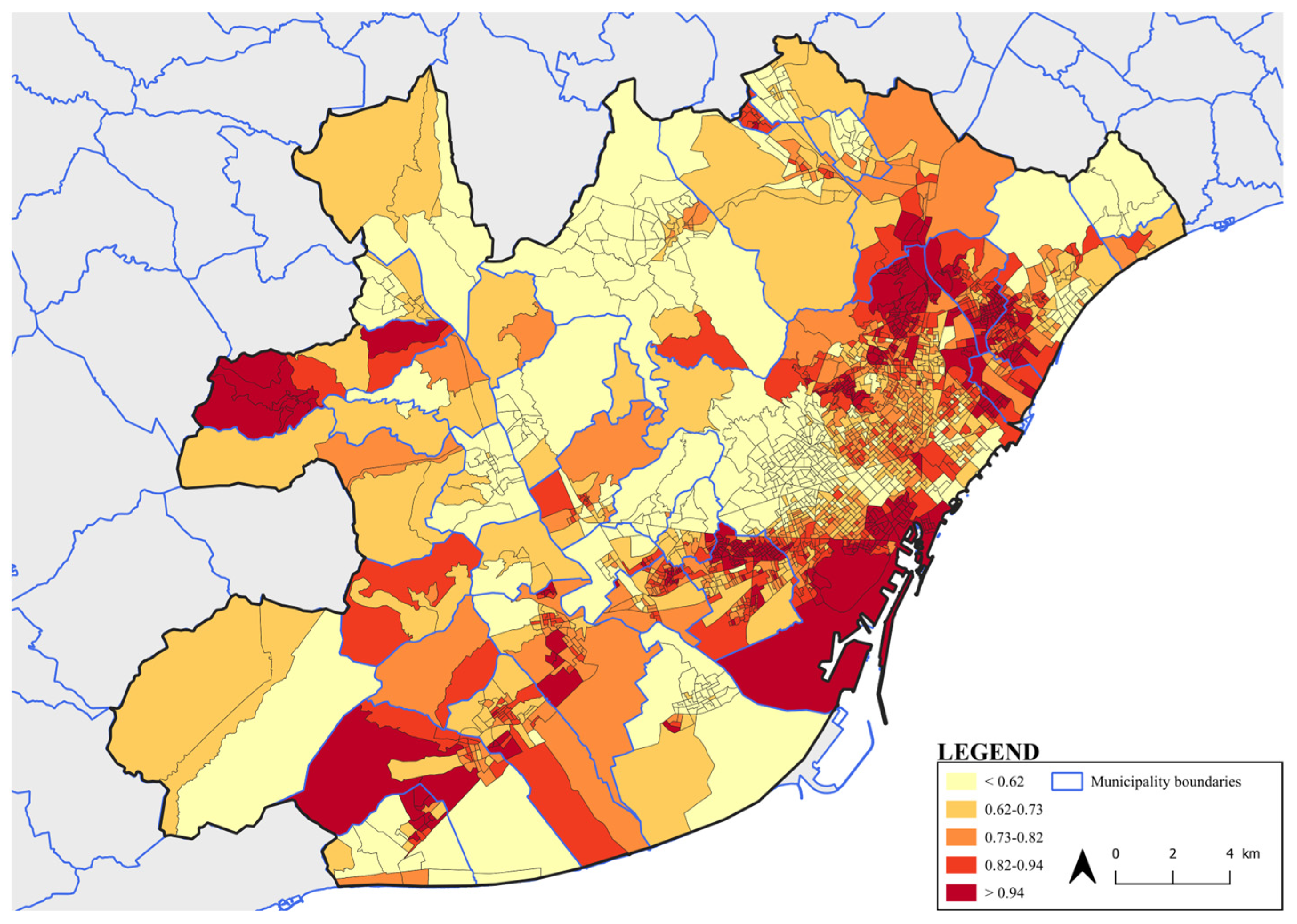
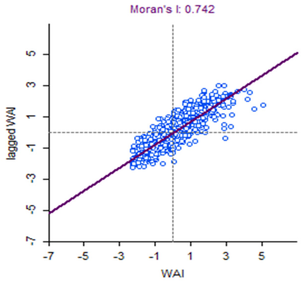
3.1. Global and Local Spatial Autocorrelation of WAI

The results of the statistical analysis regarding the spatial distribution of the WAI indicated that there was a spatial correlation of CTs having a strong and positive statistical relationship of high and low values (at a 0.05 significance level), as shown by the Global Moran’s I results (Moran’s I = 0.742) (Figure 2).
To evaluate possible heterogeneity in the data at the CT level and to locate the different patterns of autocorrelation at the local level, LISA analyses (the local version of Global Moran’s I) were conducted. The resulting LISA map (Figure 3) identified four types of CT clusters. First, CTs having a high WAI and being surrounded by CTs also having a high WAI (labelled as “High-High”). Second, CTs having a low WAI and being surrounded by CTs also having a low WAI (labelled as “Low-Low”). Third, CTs having high WAI values but that are surrounded by CTs having low WAI (labelled as “High-Low”), and fourth, CTs having low WAI but that are surrounded by CTs with high values of WAI (labelled as “Low-High”).
After applying the local Moran’s I indicator, if results were not statistically significant at the 0.05 level, CTs were excluded from the LISA map. Of the total CTs analysed, 379 CTs belonged to the High-High cluster type (18% of the total), 425 CTs to the Low-Low type (20% of the total), 11 CTs to the Low-High cluster and 13 CTs to the High-Low type (0.5 and 0.6% of the total, respectively). The remaining CTs (61%) were classified as “non-significant”. LISA clusters showed a clear spatial aggregation within different CT values for WAI (Figure 3).
The results for LISA autocorrelation shown in the LISA Map (Figure 3) enabled us to identify the CTs forming the WAI High-High clusters. These clusters mostly, but not exclusively, pertained to low-income neighbourhoods of Barcelona and other highly populated municipalities of the MAB, basically located in four areas: two in the east and northeast of the MAB; one in the Ciutat Vella or the historical downtown district of the city of Barcelona, and another one in the northern zone of l’Hospitalet de Llobregat, in the southwest of the MAB. Smaller clusters could be found in other low-income districts of Barcelona, in very dense metropolitan cities. However, one “High-High” cluster has been found in low-density and high-income suburban areas toward the west of the metropolitan area (see Corbera del Llobregat in Table A1). In contrast with High-High spatial clusters, large extensions of the MAB could be classified under the Low-Low cluster typology. These areas included some of the wealthiest districts of Barcelona in the north and northwest of the city as well as in several high-income towns of the north, northwest, southwest and extreme southeast of the MAB. However, also some of the municipalities with the lowest income in the metropolitan area are clustered in the Low-Low typology in the north of the study area (see Ripollet and Barberà del Vallès in Table A1).
It is also interesting to highlight the CTs clustered around the High-Low type. These CTs were located in municipalities with diverse socioeconomic characteristics and their clusters were small (from one to three CTs). The same trend could be found in the Low-High group.
More than 60% of the CTs had a “non-significant” statistical autocorrelation for WAI, meaning that there was no significant spatial clustering or dispersion of WAI values across the study area. As shown in (Table 1), the High-High CTs cluster group represented only 5.11 percent of the CTs of the MAB area but concentrated 17.50 percent of the total population. Approximately the same proportion of the population could be found in the Low-Low cluster which occupied, however, over a third of the MAB area.

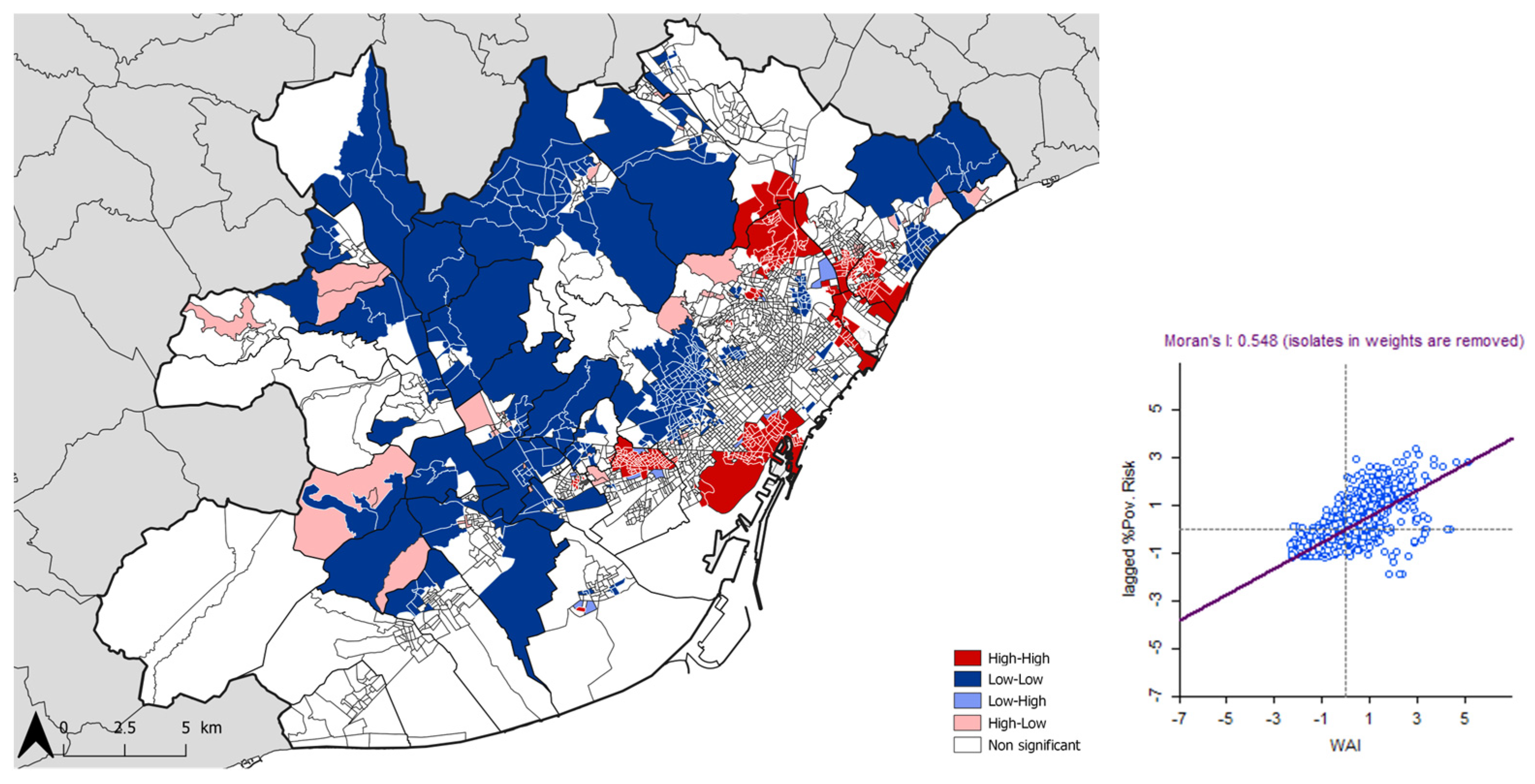
3.2. Bivariate Correlations: WAI and Population at Risk of Poverty

In the same way as in the former auto-correlation analysis (LISA), bivariate analysis (BLISA) identifies those CTs with high values for both variables (WAI and population at risk of poverty) that are surrounded by CTs with the same pattern (that is, with high values for both variables). The Bivariate Global Moran’s I at the CT level was calculated for the variables WAI and population at risk of poverty. Results indicated a moderate to strong spatial autocorrelation between these variables (Moran’s I = 0.548) in MAB municipalities (Figure 4).
High-High clusters, or spatially clustered CT with high values of both variables, were found in the four areas described in the previous section. The main differences between the WAI LISA autocorrelation map (Figure 3) and BLISA maps occurred in the Low-Low cluster type. The area occupied by this cluster type was significantly smaller in BLISA Maps (low values for both variables in clustered CTs), as some metropolitan municipalities and some northern districts of Barcelona saw most of their CTs changing to statistically “non-significant”. In these cases, therefore, no statistical similarity between those CTs and their neighbours could be found, since the variable percentage of the population at risk of poverty was also considered for each CT. However, it is important to note that the “High-High” cluster located in the western MAB low-density and high-income suburban area (Corbera del Llobregat) has also changed to “non-significant”. When we compared the WAI LISA autocorrelation map with the bivariate correlation map of the population at risk of poverty, we saw some differences that could indicate in some cases an increased vulnerability of households to water poverty vulnerability combined with high percentages of the population at risk of poverty. Accordingly, in these CTs water prices likely exerted an important influence on water affordability.

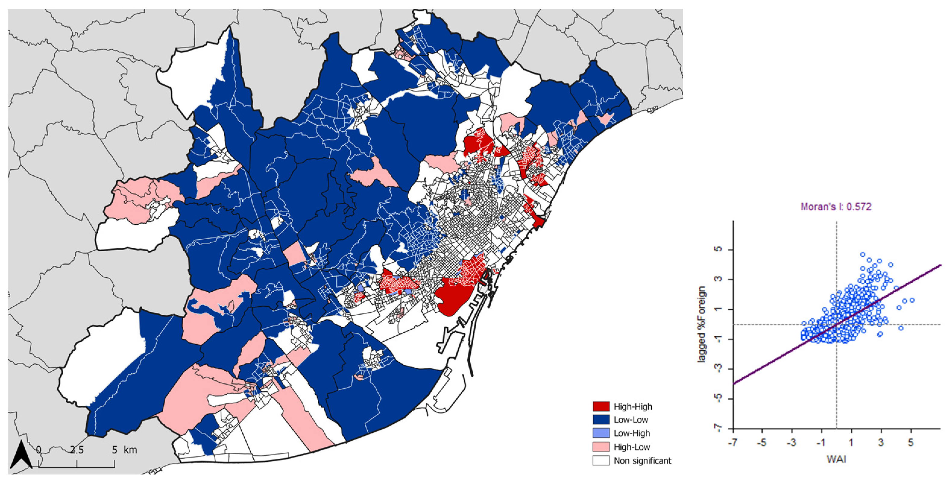
3.3. WAI, Gender and Residents Born in Global South Countries

The comparison between WAI values and the percentage of women and men (separately) at risk of poverty yielded no significant differences between women (Moran’s I = 0.519) and men (Moran’s I = 0.527) (Figure 5). In contrast, the Bivariate Global Moran’s between WAI and the percentage of the population born in countries of the Global South showed a positive and strong spatial correlation (Moran’s I = 0.572) (Figure 6). This indicated that high WAI values tended to be located close to CT having a high proportion of residents from these countries. The clusters shown on the Bivariate LISA cluster map (Figure 6) for these residents highlight similar spatial groupings. The High-High category indicated once again a spatial aggregation in the same four areas mentioned in previous sections. In this case, however, the High-High clusters included fewer CT than the WAI autocorrelation (294 vs. 379). Some of the small clusters located outside the four main areas in the WAI LISA autocorrelation map disappeared and the extension of these main clusters diminished.

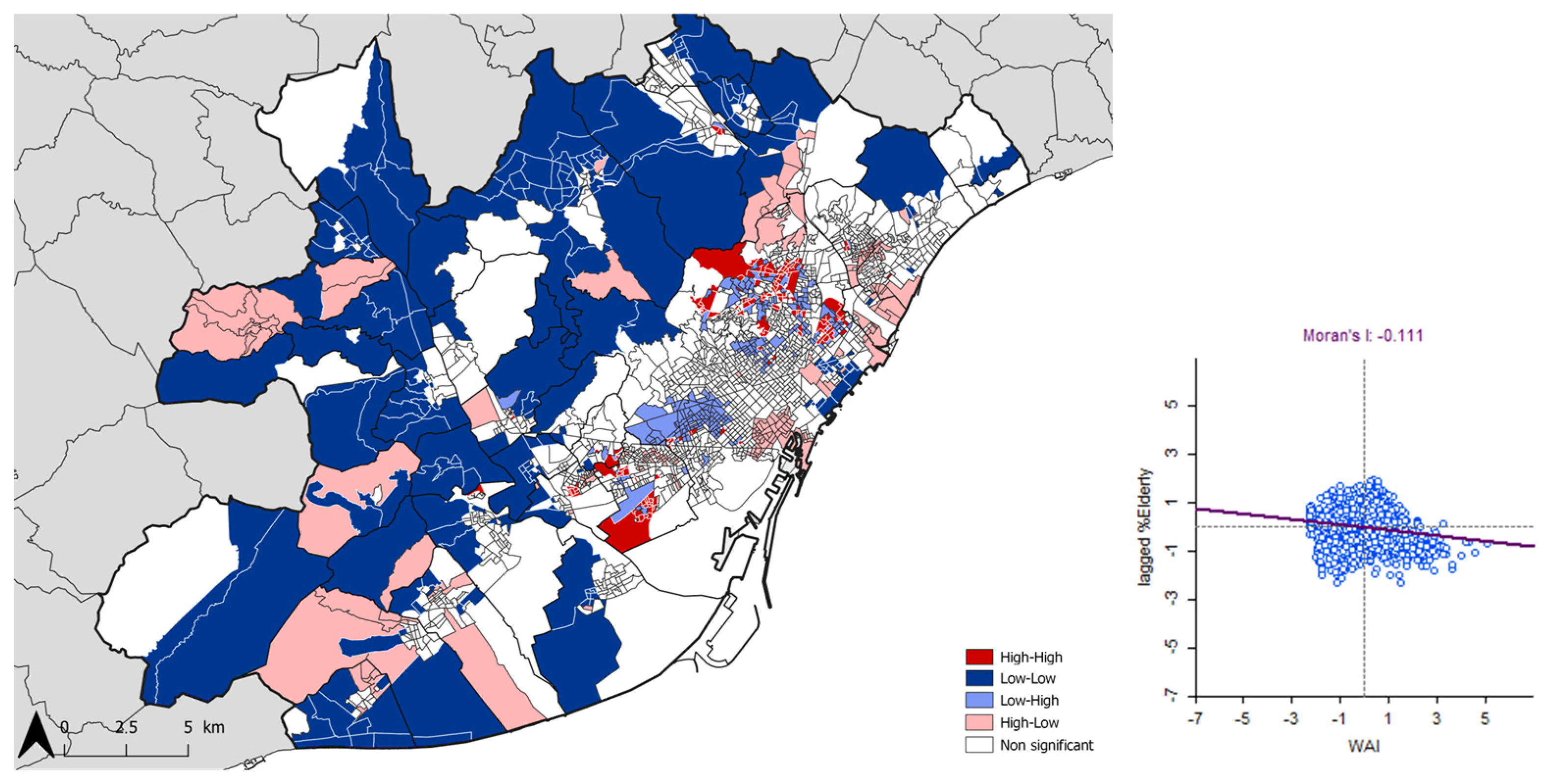
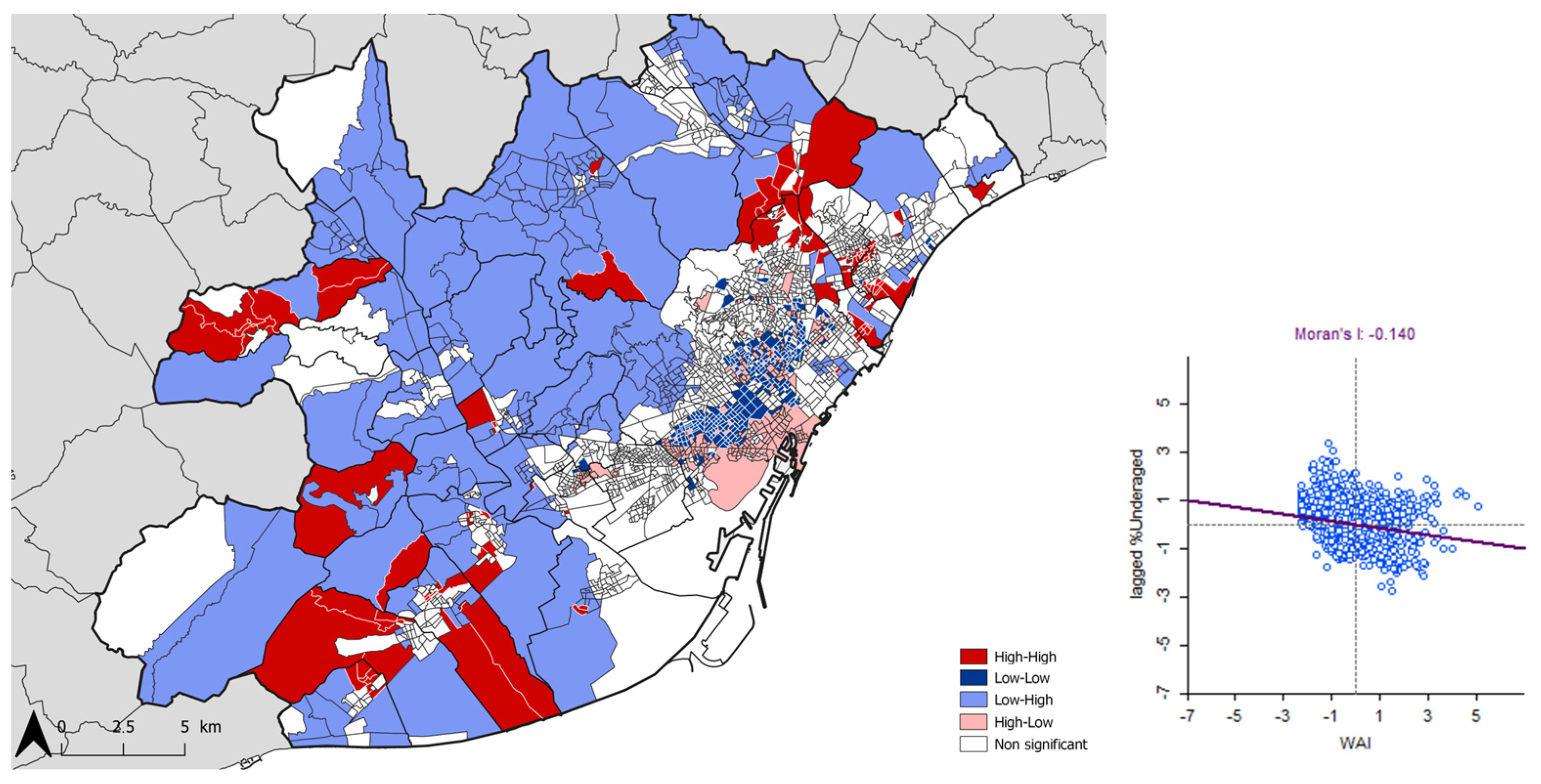
3.4. Bivariate Correlation: WAI and Percentage of Elderly and Underaged Population

The application of Bivariate Global Moran’s I at the CT level to calculate the statistical correlation between WAI and the percentage of the elderly population (over 65 years) showed a negative and weak spatial correlation (Moran’s I = −0.111) (Figure 7). Something similar occurred when we calculated the statistical correlation with the percentage of the underaged population (18 years or younger), observing also a negative and weak (Moran’s I = −0.140) but significant at the 0.05 level spatial correlation (Figure 8).
Despite this weak spatial correlation, the Bivariate LISA cluster maps (Figure 7 and Figure 8) deserve some comments. In the case of the population over 65 years (Figure 7), there was a clear correlation in the Low-Low cluster category. Most of the northern MAB areas previously categorised as Low-Low in the WAI autocorrelation found themselves in a similar situation for this variable (low WAI values and low percentage of this population group). The four main cluster areas described in the previous sections remained clustered although with lesser CTs than previously. In this case, however, all CTs changed to High-Low, indicating high values for WAI and low values for the proportion of the population 65 years old or older. Some other CTs in the same municipalities near these four main areas were categorised as High-High. Here, the most important aggregations belonged to the dense, low-income, and peripheral districts of Barcelona and its neighbouring municipalities.
In the case of the population 18 years old or younger, the Bivariate LISA cluster map (Figure 8) showed a completely different pattern. In this case, only three of the four areas mentioned previously were significant. Both clusters in the northeast were categorised as High-High, meaning that high WAI values and a high proportion of the population 18 or younger were present. In the Ciutat Vella district of Barcelona, the cluster was catalogued as High-Low, since the proportion of young people was statistically low. Most of the northern MAB municipalities and the Barcelona affluent neighbourhoods were part of the Low-High cluster typology. This situation indicated that the majority of these mostly wealthy municipalities had low WAI values and a high proportion of underaged residents, except for some specific CTs and the western cluster previously highlighted (Corbera del Llobregat), where values for WAI were also statistically High.

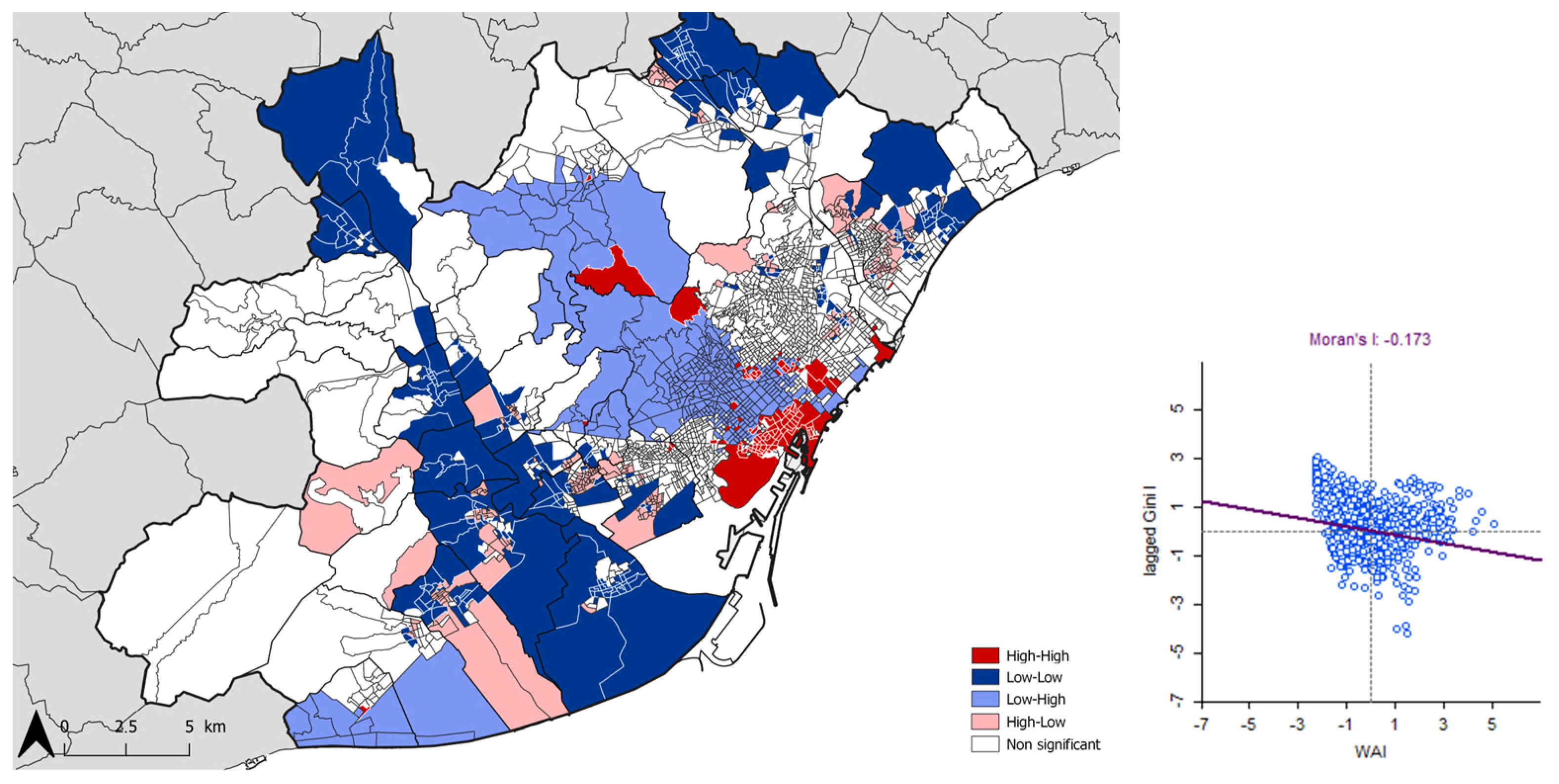
3.5. Bivariate Correlation: WAI and Gini Index

The Gini Index has been used to represent economic inequality. This Index typically ranges from 0 to 1, where 0 represents perfect equality (everyone has the same income or wealth) and 1 represents perfect inequality (one person or household has all the income or wealth, while others have none). The spatial comparison of the relations between WAI and the Gini Index produced a negative and weak correlation (Global Moran’s I = −0.173) (Figure 9). This indicated a tendency to find lower WAI values associated with higher Gini I values.
As the Bivariate LISA cluster map (Figure 9) shows, these clusters differed significantly compared to the other cluster maps. In this case, the southwest of the MAB was mostly occupied by the Low-Low CTs cluster typology, pointing at a spatial aggregation of CTs with low WAI values and less income inequality. A similar pattern could be detected in eastern and northeastern municipalities. The two municipalities having a public water supply company fell in the Low-Low category while wealthy municipalities and neighbourhoods of Barcelona city had a significant Low-High type. In the Ciutat Vella District of Barcelona, the High-High type was found in most of the area.

4. Discussion

Next, we discuss the results obtained in both methodological and empirical terms in light of the debates on water poverty. Regarding the methodology used, and especially the definition of a threshold to highlight water-poor households, and in agreement with Smets [30], Miniaci [24], and Vanhille [10], we acknowledged that, at least in the context of Western Europe, the threshold of 3 percent of household income spent on the water bill to define water poor households is too restrictive. This holds true even at relatively disaggregated scales such as CTs. Universal benchmarks are hard to establish because of the highly contextual socioeconomic conditions governing affordability [13]. Identifying water-poor households using the 3 percent threshold seems most feasible through survey methodologies that analyse households as individual units and extrapolate the findings to the desired scale, as demonstrated in the studies conducted by Martins [9] in Portugal and Domene [31] in the MAB. The main problem with the latter approach is that results are then aggregated at scales (national or regional) that do not allow precise socio-spatial assessments of the magnitude and characteristics of this type of poverty, serving as input to policy initiatives based on fine-grained analyses.
As some US-based studies have shown [13,20,21], working at the CT scale may not yield estimations of water-poor households based on a fixed relation between expenditure and income at the household level. However, working at this scale allows for the recognition of differences in the cost of essential water uses for households at a very disaggregated scale. Furthermore, this methodology may provide a clearer picture of the relationships between affordability and other sociodemographic variables related to poverty. By abandoning the 3% debate and focusing instead on comparing the water affordability index with other variables at the CT scale, we coincide with some of the results obtained in USA studies on water poverty. Water affordability may reveal important relationships not only with income but also with other sociodemographic data, most notably the population born in developing countries [13]. Likewise, we have found that variations in the economic cost of water as reflected in the bills exert a distinctive effect on affordability, especially in cases where the same and usually high water prices apply to areas with highly different income levels. In contrast with the European studies, USA studies such as that by Mack and Wrase [21] do not work with the cost of basic water requirements but with the cost of total water consumption. Considering basic needs, and although some corrections may apply, it can be argued that the spending effort made by households in low-income areas may be comparatively much larger than the equivalent for high-income households. This appears to be especially true when regional and municipal taxes are added to the bill. Thus, municipalities supplied by the same company may produce water bills that are substantially different and that may increase or decrease WAI values even in low-income metropolitan areas (Table A1). In our case, 34 out of 36 municipalities in the MAB are supplied with water from companies totally or partially private.
Our quantification of the WAI using a needs-based approach introduces a spatial dimension (CT) absent in most European work where the scale of analysis is generally national [24]; regional [10] or municipal [34]. Even performing the analysis at the metropolitan scale, figures would not suggest affordability problems for the MAB where, on average, water expenses represent 2.3 percent of household income [40]. In our study case, high WAI values were unevenly distributed across the study area (Figure 1). Spatially, the strong relationship with income was evident and expected in most cases but when considering the average size of households or, especially, the cost of water, some differences appeared. For example, the only two municipalities where water supply is managed by a public company required a smaller effort in the payment of water bills. For a monthly consumption of 8 m3, the water cost in these two municipalities represented 66 percent of the water cost of the municipality of Barcelona (EUR 1.7/m3 and EUR 2.57/m3, respectively). On the opposite side, in certain peripheries of the MAB, some municipalities recorded higher WAI values than expected according to their income. In the most extreme case, water was managed privately, and the cost rose to EUR 3.46/m3.
Local Spatial Autocorrelation Analysis allowed for the identification of CTs spatially clustered by WAI values and identified the areas where the index of essential water affordability was higher, indicating a higher spending effort reflected in the water bill. Even though most of the High-High WAI autocorrelation clusters were mostly located in high-density, historically deprived cities and neighbourhoods, we could also appreciate some clusters located in wealthier municipalities due to high water prices (see Table A1). Most of the High-High-clustered low-income neighbourhoods were built between the 1950s and the 1970s to accommodate the thousands of families from other regions of Spain arriving in the Barcelona Metropolitan Area. Decades later they became the home for many of the Global South immigrants arriving in the area since the year 2000. In 80 percent of the High-High CTs, the population density stands above 25,000 inh./km2. This population usually live in small flats in high-rise residential buildings, conforming to the low water consumption pattern characteristic of this urban model [27]. Average municipal per capita water consumption in these areas usually falls below the 100 lpd threshold, with consumptions as low as 92.9 lpd, and often around 95 lpd [48]. These quantities mean that at least, part of the population in the four areas with high WAIs might not be fulfilling entirely its basic water needs as determined by the 100 lpd threshold. Thus, our results can be compared with those of Vanhille [10] in that we do not only provide an indication of water affordability but also give an indication of the population with consumptions below the threshold of 100 lpd. Finally, we compared some of our results with those of the European Survey of Income and Living Conditions for the specific case of the Metropolitan Region of Barcelona [31,32]. According to survey results in the MAB, on average, 2.35 percent of household income went to pay for the satisfaction of minimum water requirements, but in households at risk of poverty, this proportion jumped to 7.46%. Surveys may offer a more precise picture of the extent of water poverty in the area [8] but cannot be meaningfully extrapolated to the municipal or submunicipal level within the MAB.
All bivariate correlations provided additional information on the relationships between water affordability and sociodemographic vulnerability. When comparing WAI with variables such as the percentage of the population at risk of poverty or the percentage of the population coming from Global South countries, the spatial correlations were strong and positive. These results concurred with data from recent reports stating that almost half of foreign-born Spanish residents lived under precarious economic conditions. This proportion is twice the equivalent for those born in Spain [36]. Comparing High-High CTs (high values for WAI and high social vulnerability) with the WAI autocorrelation map (Figure 3), similar cluster areas were generated. In fact, of the 294 CTs categorised as High-High in the WAI spatial autocorrelation, 231 were also categorised as High-High in the bivariate spatial correlation analyses (population at risk of poverty and population born in developing countries) (Figure 3). Those 231 CTs concentrate more than 357,000 people or about 11 percent of the population of the MAB. Therefore, the water affordability index developed in this research was useful for locating, at a highly disaggregated spatial scale, areas in which social and economic deprivation is related to water affordability, showing how the distribution pattern of low affordability does not occur randomly but tends to cluster in areas already suffering from poverty conditions [13,49,50] and with average municipal water consumptions per capita below 100 lpd.
Regarding relationships between the WAI and age, in both groups (65 years or more and 18 years or less) correlations were weaker but still statistically significant. The results obtained show diverse demographic realities in the metropolitan area. Thus, the spatial bivariate correlation map between WAI and the percentage of the underaged population (Figure 8) reflected the higher percentages of this population group at both ends of the social spectrum. The demographic cohorts of young people were more present in low-income areas heavily populated by immigrants but also in the affluent districts and especially suburbs of Barcelona where the number of young professionals with children is growing. The same pattern could be found in the districts of Barcelona where the proportion of the underaged population in the more affluent areas tended to be higher than in certain traditional middle- and lower-class neighbourhoods and suburbs increasingly dominated by older demographic groups [31]. Regarding the Gini Index, the spatial correlation obtained showed a weak and negative correlation, which concurs with the trend that differences in income tend to be higher in higher-income areas than in lower-income areas. From the BLISA map (Figure 9) comparison with the LISA map (Figure 3), only the historical downtown district of Barcelona showed a statistically significant High-High cluster meaning that in these CTs economic inequality is high. This was probably caused by gentrification processes common to old and degraded areas in certain European historical city centres [51].
It is also important to mention some limitations of the study. First, although CTs are the most disaggregated scale for which data could be obtained, it is still an aggregated unit that may hide extreme values. Second, it would have been more convenient in the calculation of the WAI to use as income the average income of the population at risk of poverty (i.e., population with an income of 60% or less than the average income of the MAB). However, as explained in the text, this has not been possible due to the peculiar structure of Spanish statistics in this regard. The selection of 100 lpd as representative of the quantity able to fulfil essential uses is also open to criticism because, among other problems, it ignores economies of scale in water consumption. Finally, some households with difficulties in paying their water bills are benefitting from subsidies by the water companies or local/regional governments influencing in this way affordability issues. Some issues remain for future work such as, for example, the possibility of considering the cost of bottled water (highly present in many low-income households) in affordability estimates; the need to attend to the specific cases of households with members sick or disabled, and the effects of the introduction of subsidies to attenuate the impacts of high water costs.

5. Conclusions

This paper has evaluated water affordability for essential uses in the Metropolitan Area of Barcelona with the aim of assessing its relevance and relationships with poverty-related variables. The main contributions of the paper can be summarised as follows. First, in the literature review, we noticed a certain “Atlantic divide” between European studies using a basic needs approach for estimating household expenditures on water, and North American studies in which the use of total water expenditure is more common. In contrast, US-based studies provide a much more spatially detailed analysis of water affordability than European contributions, taking advantage of the rich data historically available at disaggregated scales such as CT. Our study attempts to bridge both approaches in that we use the basic needs approach and perform our analysis at the scale of the CT even though the data available are not as complete as in the USA cases. Some data at this scale may be difficult to obtain. However, national statistical services, at least in most European countries, are increasingly able to provide basic sociodemographic information at small scales. In this regard, our study might be one of the first to use spatially disaggregated units to investigate water affordability in Europe. Second, and in line with the US contributions we have also provided results at the scale of the CTs on the relations between water affordability and several sociodemographic variables common in the studies on poverty such as income and income inequality, population born in countries of the Global South, or age. Third, following American and some European references [9,19,30] we have stressed the important role of water prices in determining affordability. Some contributions tend to emphasise the income variable, deflecting the attention away from prices. Water prices and the myriad of other items included in the water bills of households in the Metropolitan Area of Barcelona rose significantly during the decade after the economic crisis beginning in 2007 amid growing unemployment and general income stagnation or decline. In this respect, the WAI indicator may also be used to simulate the effects of alternative, more just tariff structures on water affordability. Moreover, our study could help in designing public policies more attentive to correct high water costs at least for the more vulnerable households. Finally, we may also conclude that the selection of a universal threshold such as 3 percent of available income to calculate and identify water-poor households is very problematic and probably of little practical use due to several reasons such as the highly contingent nature of data aggregation. Therefore, studies on vulnerability to water poverty may find useful methodologies such as the one employed in this study.

Author Contributions

Conceptualisation, G.R.-G., E.D. and D.S.; methodology, G.R.-G. and X.G.; software, G.R.-G. and X.G.; validation, E.D., H.Y. and D.S.; formal analysis, G.R.-G.; investigation, D.S. and G.R.-G.; writing, G.R.-G. and D.S.; review, D.S., X.G. and E.D.; project administration, D.S.; funding acquisition, G.R.-G. and D.S. All authors have read and agreed to the published version of the manuscript.

Funding

This research was funded by the Ministry of Science, Innovation and Universities, Spain (PRE2020-094096 and PID2019-104456RB-C21).

Data Availability Statement

The raw data supporting the conclusions of this article will be made available by the authors on request.

Conflicts of Interest

The authors declare no conflicts of interest.

Appendix A

Table A1. Results obtained for each municipality in MAB area.
MunicipalityTotal PopulationAverage Household Income (EUR/Year)Supply CompanyAverage Essential Water Spending (EUR/Year)Average WAI (%)CTs with WAI Values Higher than MAB Average Values (%)Population Living in CTs with WAI Values Higher than MAB Average Value (%)
MAB3,222,65437,546-273.730.794743.66
Badalona218,53831,745ABEMCIA251.200.845955.30
Badia Del Vallès13,38727,367SOREA242.760.89100100
Barberà Del Vallès32,74535,670Aigües de Barberà *207.190.5900
Barcelona1,595,74739,678ABEMCIA279.400.774140.51
Begues706551,243ABEMCIA338.470.6600
Castellbisbal12,35939,231AICSA242.000.6200
Castelldefels65,71145,091ABEMCIA320.880.785042.98
Cerdanyola Del Vallès56,69340,866ABEMCIA268.580.702726.27
Cervelló883743,271SOREA298.290.6900
Corbera De Llobregat14,52543,474SOREA418.640.999193.08
Cornellà Del Llobregat87,89832,062ABEMCIA267.690.866755.57
Esplugues De Llobregat46,19443,493ABEMCIA272.390.702829.79
Gavà46,55736,683ABEMCIA284.870.806153.80
Hospitalet De Llobregat262,36530,249ABEMCIA270.930.927776.83
La Palma De Cervelló291741,991ACAT251.470.6000
Molins De Rei25,79539,164AQUALIA201.100.5200
Montcada I Reixac35,85133,440ABEMCIA273.270.845050.12
Montgat11,97038,078ABEMCIA286.350.762526.69
Pallejà11,27542,475ABEMCIA277.400.6700
El Papiol413139,581ABEMCIA273.530.7000
El Prat De Llobregat63,86734,337Aigües del Prat *199.980.6053.95
Ripollet38,56131,763SOREA190.530.6100
Sant Adrià De Besòs36,74528,854ABEMCIA279.491.037973.04
Sant Andreu De La Barca27,18335,553AQUALIA211.460.6000
Sant Boi De Llobregat82,72533,671ABEMCIA269.390.825450.47
Sant Climent De Llobregat410740,511ABEMCIA322.620.805046.72
Sant Cugat Del Vallès88,96661,718SOREA323.680.56105.83
Sant Feliu De Llobregat44,43037,825ABEMCIA270.760.744030.43
Sant Joan Despí33,89240,022ABEMCIA272.360.703628.22
Sant Just Desvern17,28760,551ABEMCIA268.130.48115.32
Santa Coloma De Cervelló809343,866ABEMCIA291.090.6700
Santa Coloma De Gramanet117,93428,497ABEMCIA280.731.019392.36
Sant Vicenç Dels Horts27,68134,501SVH181.390.5300
Tiana871656,547SOREA272.950.4900
Torrelles De Llobregat597842,174ABEMCIA323.060.775041.45
Viladecans66,14435,706ABEMCIA276.960.795349.47
Note: * Public management.

References

  1. United Nations General Assembly (UN). The Human Right to Water and Sanitation: Resolution/Adopted by the General Assembly. Available online: https://www.refworld.org/legal/resolution/unga/2010/en/76535 (accessed on 22 February 2024).
  2. Langford, M. The United Nations Concept of Water as a Human Right: A New Paradigm for Old Problems? Int. J. Water Resour. Dev. 2005, 21, 273–282. [Google Scholar] [CrossRef]
  3. Anand, P.B. Right to water and access to water: An assessment. J. Int. Dev. 2007, 19, 511–526. [Google Scholar] [CrossRef]
  4. Pérez-Foguet, A. Broadening the Water Affordability Approach to Monitor the Human Right to Water. Cities 2023, 143, 104573. [Google Scholar] [CrossRef]
  5. United Nations General Assembly (UN). Transforming Our World: The 2030 Agenda for Sustainable Development. Available online: https://www.refworld.org/legal/resolution/unga/2015/en/111816 (accessed on 15 July 2023).
  6. Meehan, K.; Jepson, W.; Harris, L.M.; Wutich, A.; Beresford, M.; Fencl, A.; London, J.; Pierce, G.; Radonic, L.; Wells, C.; et al. Exposing the Myths of Household Water Insecurity in the Global North: A Critical Review. WIREs Water 2020, 7, e1486. [Google Scholar] [CrossRef]
  7. Ezbakhe, F.; Giné-Garriga, R.; Pérez-Foguet, A. Leaving No One behind: Evaluating Access to Water, Sanitation and Hygiene for Vulnerable and Marginalized Groups. Sci. Total Environ. 2019, 683, 537–546. [Google Scholar] [CrossRef] [PubMed]
  8. Yoon, H.; Domene, E.; Sauri, D. Assessing Affordability as Water Poverty in Metropolitan Barcelona. Local Environ. 2021, 26, 1330–1345. [Google Scholar] [CrossRef]
  9. Martins, R.; Quintal, C.; Cruz, L.; Barata, E. Water Affordability Issues in Developed Countries—The Relevance of Micro Approaches. Util. Policy 2016, 43, 117–123. [Google Scholar] [CrossRef]
  10. Vanhille, J.; Goedemé, T.; Penne, T.; Van Thielen, L.; Storms, B. Measuring Water Affordability in Developed Economies. The Added Value of a Needs-Based Approach. J. Environ. Manag. 2018, 217, 611–620. [Google Scholar] [CrossRef]
  11. Goddard, J.J. Measuring Drinking Water Affordability and Sustainability; UC Berkeley: Berkeley, CA, USA, 2019. [Google Scholar]
  12. Sullivan, C.; Meigh, J. Considering the Water Poverty Index in the Context of Poverty Alleviation. Water Policy 2003, 5, 513–528. [Google Scholar] [CrossRef]
  13. Goddard, J.J.; Ray, I.; Balazs, C. Water Affordability and Human Right to Water Implications in California. PLoS ONE 2021, 16, e0245237. [Google Scholar] [CrossRef]
  14. Petrova, S.; Simcock, N. Gender and Energy: Domestic Inequities Reconsidered. Soc. Cult. Geogr. 2021, 22, 849–867. [Google Scholar] [CrossRef]
  15. Middlemiss, L. Who Is Vulnerable to Energy Poverty in the Global North, and What Is Their Experience? WIREs Energy Environ. 2022, 11, e455. [Google Scholar] [CrossRef]
  16. Oliveras, L.; Artazcoz, L.; Borrell, C.; Palència, L.; López, M.J.; Gotsens, M.; Peralta, A.; Marí-Dell’Olmo, M. The Association of Energy Poverty with Health, Health Care Utilisation and Medication Use in Southern Europe. SSM-Popul. Health 2020, 12, 100665. [Google Scholar] [CrossRef] [PubMed]
  17. Galvin, R. Letting the Gini out of the Fuel Poverty Bottle? Correlating Cold Homes and Income Inequality in European Union Countries. Energy Res. Soc. Sci. 2019, 58, 101255. [Google Scholar] [CrossRef]
  18. Fagundes, T.S.; Marques, R.C.; Malheiros, T. Water Affordability Analysis: A Critical Literature Review. AQUA-Water Infrastruct. Ecosyst. Soc. 2023, 72, 1431–1445. [Google Scholar] [CrossRef]
  19. Teodoro, M.P. Measuring Household Affordability for Water and Sewer Utilities. J. AWWA 2018, 110, 13–24. [Google Scholar] [CrossRef]
  20. Teodoro, M.P.; Saywitz, R.R. Water and Sewer Affordability in the United States: A 2019 Update. AWWA Water Sci. 2020, 2, e1176. [Google Scholar] [CrossRef]
  21. Mack, E.A.; Wrase, S. A Burgeoning Crisis? A Nationwide Assessment of the Geography of Water Affordability in the United States. PLoS ONE 2017, 12, e0169488. [Google Scholar] [CrossRef] [PubMed]
  22. Bradshaw, J.; Huby, M. Water Poverty in England and Wales. J. Poverty Soc. Justice 2013, 21, 137–148. [Google Scholar] [CrossRef]
  23. Reynaud, A. Assessing the Impact of Public Regulation and Private Participation on Water Affordability for Poor Households: An Empirical Investigation of the French Case; LERNA, University of Toulouse: Toulouse, France, 2006. [Google Scholar]
  24. Miniaci, R.; Scarpa, C.; Valbonesi, P. Measuring the Affordability of Basic Public Utility Services in Italy. G. Degli Econ. Ann. Econ. 2008, 67, 185–230. [Google Scholar]
  25. March, H.; Garcia, X.; Domene, E.; Saurí, D. Tap Water, Bottled Water or In-Home Water Treatment Systems: Insights on Household Perceptions and Choices. Water 2020, 12, 1310. [Google Scholar] [CrossRef]
  26. March, H.; Saurí, D. When Sustainable May Not Mean Just: A Critical Interpretation of Urban Water Consumption Decline in Barcelona. Local Environ. 2017, 22, 523–535. [Google Scholar] [CrossRef]
  27. Domene, E.; Saurí, D. Urbanisation and Water Consumption: Influencing Factors in the Metropolitan Region of Barcelona. Urban Stud. 2006, 43, 1605–1623. [Google Scholar] [CrossRef]
  28. Yoon, H.; Saurí, D. ‘No More Thirst, Cold, or Darkness!’—Social Movements, Households, and the Coproduction of Knowledge on Water and Energy Vulnerability in Barcelona, Spain. Energy Res. Soc. Sci. 2019, 58, 101276. [Google Scholar] [CrossRef]
  29. Fankhauser, S.; Tepic, S. Can Poor Consumers Pay for Energy and Water? An Affordability Analysis for Transition Countries. Energy Policy 2007, 35, 1038–1049. [Google Scholar] [CrossRef]
  30. Smets, H. Quantifying the Affordability Standard: A Comparative Approach. In The Human Right to Water: Theory, Practice and Prospects; Russell, A.F.S., Langford, M., Eds.; Cambridge University Press: Cambridge, UK, 2017; pp. 225–275. ISBN 978-0-511-86260-1. [Google Scholar]
  31. Domene, E.; Garcia, X.; Garcia, M. La Pobresa Hídrica i Energètica a L’àrea Metropolitana de Barcelona; Institut Metropoli: Barcelona, Spain, 2018. [Google Scholar]
  32. National Statistical Institute of Spain (INE); Méndez Martín, J.M. The Spanish Survey of Living Conditions (ES-SILC). Characteristics and Methodological Development. Span. J. Stat. 2019, 1, 41–56. [Google Scholar] [CrossRef]
  33. Gleick, P.H. Basic Water Requirements for Human Activities: Meeting Basic Needs. Water Int. 1996, 21, 83–92. [Google Scholar] [CrossRef]
  34. García-Valiñas, M.A.; Martínez-Espiñeira, R.; González-Gómez, F. Affordability of Residential Water Tariffs: Alternative Measurement and Explanatory Factors in Southern Spain. J. Environ. Manag. 2010, 91, 2696–2706. [Google Scholar] [CrossRef]
  35. Bartram, J.; Howard, G. 14—Drinking-Water Standards for the Developing World. In Handbook of Water and Wastewater Microbiology; Mara, D., Horan, N., Eds.; Academic Press: London, UK, 2003; pp. 221–240. ISBN 978-0-12-470100-7. [Google Scholar]
  36. Fernández Maíllo, G. VIII Informe Sobre Exclusión y Desarrollo Social en España 2019; Fundación FOESSA Cáritas española editores: Madrid, Spain, 2019; ISBN 978-84-8440-772-0. [Google Scholar]
  37. Oficina de los Consumidores (OCU). Precio del Agua en España. Available online: https://www.ocu.org/alimentacion/agua/informe/el-precio-del-agua (accessed on 5 December 2023).
  38. Porcel, S. Desigualdad Social y Segregación Residencial: Una Relación Compleja; Fundación Foessa: Madrid, Spain, 2020; ISBN 978-84-8440-823-9. [Google Scholar]
  39. Institut Metròpoli (IERMB). La Metròpoli (Post)-COVID: Impactes, Escenaris i Reptes. (Post-COVID Metropolis: Impacts, Scenarios and Challenges). Anuari Metropolità de Barcelona 2020. Available online: https://www.institutmetropoli.cat/ca/anuari/metropoli-post-covid-impactes-escenaris-reptes/ (accessed on 12 November 2023).
  40. Institut Metròpoli (IERMB). Cap a la Metròpoli 2030. Reptes Emergents, Coneixements Innovadors. (Towards the Metropolis 2030. Emerging Challenges, Innovative Knowledge). Anuari Metropolità de Barcelona 2021. Available online: https://www.institutmetropoli.cat/ca/anuari/anuari-2021/ (accessed on 7 January 2024).
  41. Agència Catalana de l’Aigua (ACA). Preu per Municipis i Evolució (Municipal Water Prices and Trends). Available online: http://aca.gencat.cat/ca/laca/observatori-del-preu-de-laigua/Preu-per-municipis-i-evolucio/ (accessed on 9 February 2024).
  42. Eurostat Database General and Regional Statistics. Available online: https://ec.europa.eu/eurostat/data/database (accessed on 7 January 2024).
  43. Instituto Nacional de Estadística (INE). (National Statistics Institute) Censo de Población y Viviendas 2021 (Populations and Housing Census 2021). Available online: https://www.ine.es/dynt3/inebase/es/index.htm?padre=9805&capsel=9809 (accessed on 15 February 2024).
  44. Anselin, L.; Syabri, I.; Kho, Y. GeoDa: An Introduction to Spatial Data Analysis. In Handbook of Applied Spatial Analysis: Software Tools, Methods and Applications; Fischer, M.M., Getis, A., Eds.; Springer: Berlin/Heidelberg, Germany, 2010; pp. 73–89. ISBN 978-3-642-03647-7. [Google Scholar]
  45. Anselin, L. An Introduction to Spatial Data Science with GeoDa: Volume 1: Exploring Spatial Data; Chapman and Hall/CRC: New York, NY, USA, 2024; ISBN 978-1-00-327491-9. [Google Scholar]
  46. Benito, B.; Guillamón, M.-D.; Ríos, A.-M. Public Management Versus Private Management in the Provision of Drinking Water: What Is the Cheapest? Lex Localis-J. Local Self-Gov. 2018, 16, 271–292. [Google Scholar] [CrossRef]
  47. Porcher, S.; Saussier, S. Public Versus Private Management in Water Public Services: Taking Stock, Looking Ahead. SSRN Electron. J. 2018, 64, 4–31. [Google Scholar] [CrossRef]
  48. Tarifas de Suministro—Web Oficial—La Gestió Responsible. Available online: https://www.aiguesdebarcelona.cat/es/servicio-agua/factura-y-tarifas-agua/tarifas-de-suministro (accessed on 15 April 2024).
  49. Gutiérrez, A.; Delclòs, X. The Uneven Distribution of Evictions as New Evidence of Urban Inequality: A Spatial Analysis Approach in Two Catalan Cities. Cities 2016, 56, 101–108. [Google Scholar] [CrossRef]
  50. Gaber, N.; Silva, A.; Lewis-Patrick, M.; Kutil, E.; Taylor, D.; Bouier, R. Water Insecurity and Psychosocial Distress: Case Study of the Detroit Water Shutoffs. J. Public Health 2021, 43, 839–845. [Google Scholar] [CrossRef] [PubMed]
  51. Anguelovski, I.; Connolly, J.J.T.; Masip, L.; Pearsall, H. Assessing Green Gentrification in Historically Disenfranchised Neighborhoods: A Longitudinal and Spatial Analysis of Barcelona. Urban Geogr. 2018, 39, 458–491. [Google Scholar] [CrossRef]
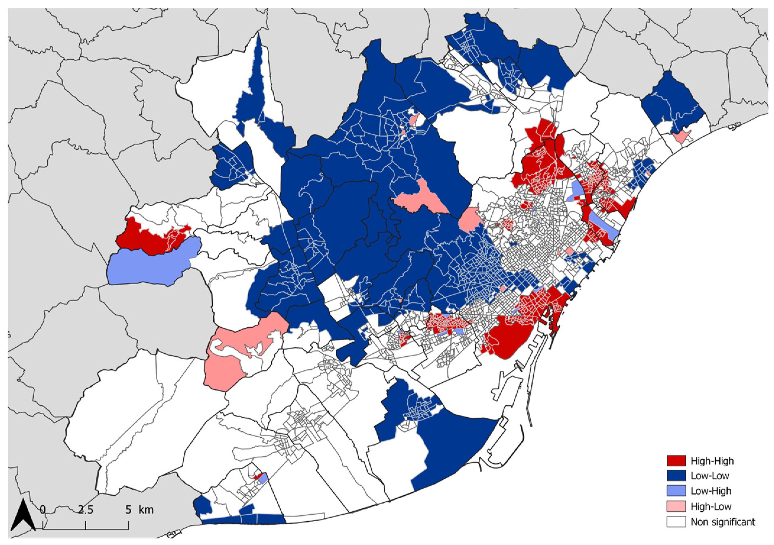
Figure 1. Distribution of the Water Affordability Index in the Metropolitan Area of Barcelona for the year 2018. The variable values are represented in quintiles.
Water 16 01496 g001
Figure 2. Global Moran’s I univariate scatter plot for WAI.
Water 16 01496 g002
Figure 3. Univariate LISA cluster map for WAI.
Water 16 01496 g003
Figure 4. WAI and population at risk of poverty BLISA cluster map and scatter plot.
Water 16 01496 g004
Figure 5. Global Moran’s I bivariate scatter plot for Gender and Water Affordability Index: (a) % of men at poverty risk and WAI; (b) % of women at poverty risk and WAI.
Water 16 01496 g005
Figure 6. WAI and percentage of population born in Global South countries BLISA cluster map and scatter plot.
Water 16 01496 g006
Figure 7. WAI and percentage of elderly (>65 years) population BLISA cluster map and scatter plot.
Water 16 01496 g007
Figure 8. WAI and percentage of underaged (<18 years) population BLISA cluster map and scatter plot.
Water 16 01496 g008
Figure 9. WAI and Gini Index BLISA cluster map and scatter plot.
Water 16 01496 g009
Table 1. LISA Autocorrelation Clusters summary for WAI variable.
Cluster CategoryMAB CTs (%)MAB Surface (%)Population (Inhabitants)Population (%)
High-High17.745.11563,56917.50
Low-Low19.8933.62691,15521.46
Low-High0.521.8719,8610.62
High-Low0.612.3318,8130.58
Non-significant61.2557.071,926,65359.83
Disclaimer/Publisher’s Note: The statements, opinions and data contained in all publications are solely those of the individual author(s) and contributor(s) and not of MDPI and/or the editor(s). MDPI and/or the editor(s) disclaim responsibility for any injury to people or property resulting from any ideas, methods, instructions or products referred to in the content.

