Optimization of Elbow Draft Tubes for Variable Speed Propeller Turbine

Abstract

The design of the elbow draft tubes is challenging due to the complexity of the flow. The whole turbine unit’s power output strongly depends on the draft tube function, especially for the low-head turbines. The article presents a novel approach to optimizing elbow draft tubes for a variable-speed propeller turbine designed for low-head applications. First, the study addresses the specifics of the propeller variable speed turbine by comparing the classical Kaplan turbine. Then, the grid scaling test is conducted to evaluate the uncertainty of the pressure regeneration. Further, a new approach to parameterising the elbow draft tube geometry is introduced. The study employs ANSYS CFX 2021 R1 software for numerical simulation to optimise the elbow draft tube geometry in the CAESES environment. After the sensitivity test and deselecting the non-sensitive parameters, we perform multi-objective genetic algorithm (MOGA) optimization. The optimization process results in a Pareto front of optimised elbow draft tube shapes with the best pressure regeneration for different draft tube construction heights, enabling the selection of suitable candidates for various locations. Minimal difference in the performance of the selected elbow draft tube shapes with the simple straight draft tube confirms a high-quality draft tube optimization achievement.

1. Introduction

Thanks to modern methods such as numerical optimization, large water turbines’ peak efficiencies are approaching physical limits, and researchers are mainly improving efficiencies in a wide range of operating points [1,2]. In the area of small hydro and especially micro hydro, the situation is slightly different. In addition to the efficiency of the machines and the power output, it is necessary to look at several criteria, such as mechanical simplicity and cost-effective solutions. For this reason, a fixed-blade propeller turbine with variable revolutions was developed for low heads (approx. up to 10 m) regulated by guide vane control and the variable speed of a runner [3,4]. Variable speed propeller turbine is mechanically simpler than the Kaplan turbine and, at the same time, allows for good discharge regulation. In this article, we will deal with optimizing the elbow draft tube (EDT) for this turbine and its specifics. The performance and efficiency of the turbine, especially of the low-head turbine, greatly depend on the properties of the draft tube (DT). The main goal of the draft tube is to convert residual kinetic energy back into pressure and minimize the hydraulic losses in the draft and the energy losses at the exit profile [5]. According to Mosonyi [6], the kinetic energy that can be turned back into pressure can reach up to 50% of the total energy for turbines with extra high specific speeds n_q (extra low heads). Simultaneously, the importance of the DT increases for discharges greater than discharge in the point with the highest efficiency BEP [7].

For a straight conical draft tube (SDT), the shape is clearly defined. Various types of DTs were historically used for vertical turbine units (e.g., hydraucone, Moody’s DT [8]). Today, elbow draft tubes (EDTs) are exclusively used for vertical turbines, although often with an inappropriate shape that needs to be adjusted (e.g., sharp-heeled EDT [9]). The EDT is basically a divergent tube with a change of centreline from vertical to horizontal, where the circular inlet profile (exit profile of the runner chamber) transitions to the rectangular cross-section of the outlet profile of the DT. The efficient conversion of kinetic energy depends on the shape of the velocity field at the entrance to the DT and the shape of the DT itself. Each DT is, therefore, original in itself, and for a high-quality DT design, it is necessary to use CFD assessment and better optimization.

With the gradual development of CFD tools and computer technology, it is possible to perform not only routine steady-state RANS calculations but also more demanding unsteady simulations using turbulent models solving a more significant portion of the turbulent spectrum—SAS, LES, DES [5]. These days, unsteady calculations of fewer design points (geometries) are possible [10]. However, in optimization loops where hundreds or thousands of calculations must be performed, it is incredibly time-consuming to use a more advanced approach to calculate a more significant part of the turbulent spectrum. Steady-state RANS calculations are still the only way to offer relatively high-quality results with less computational effort [9]. Most authors optimize DT for the operation of the given turbine unit—for a single operation point [11,12,13] or for multiple operation points [14]. The key for multiple operation points optimization, is to assign weight to each operating point, which is understandable for optimisation where hydrological parameters are known. There are also authors such as Ciocan et al. [15] who deal with how the velocity field at the DT inlet should look to improve DT behaviour. End goal optimisation is simultaneously optimizing the runner and the DT [2]. However, this method requires high-performance hardware, and at the same time, it is necessary to significantly limit the number of parameters defining the shapes of the runner and DT so that the design space would not be too large.

The velocity field at the exit from the runner is often taken from a detailed CFD simulation of the entire turbine with the primary conical draft tube due to the limited computing resources. Several authors confirm the reliability of this method for optimisation [11,14,16].

When optimizing draft tubes in general, genetic algorithms are probably used the most. There are usually more objective functions—these algorithms are called MOGA (Multi-objective genetic algorithms). McNabb et al. [14] address the use of genetic algorithms in the optimization of draft tubes. The disadvantage of using genetic algorithms is the evaluation of a large number of variants and, thus, the total computing time. Lyutov et al. [2] reported that the entire optimization process consisted of 60 generations, each generation having 120 individuals. In total, there were 7200 calculations.

The use of surrogate models in the optimisation of draft tubes is not yet very widespread. Exceptions are the doctoral thesis of D. Marjavaar [17], article by Demirel et al. [18] or Sikirica et al. [19]. Recently, publications using response surface methodology have appeared more frequently for the optimisation of the draft tubes. Let us mention here, for example, the paper of Orso et al. [12]. In the early stages of our work, however, we discovered that the style of our optimisation (respectively, parameterisation of EDT geometry) does not allow the use of surrogate models since the correlations of individual input parameters (defining the geometry) and objective functions are close to zero. Thus, we proceeded without surrogate models, using MOGA optimisation and creating a final set of the best candidates (Pareto front).

2. Paper Overview

The presented article focuses on optimizing the EDT of a propeller turbine with double regulation by guide vanes and the variable speed of a runner. This particular turbine was previously optimised for a unit runner (1-m diameter) with a gross head equal to 4 m [4]. In this mentioned article, the optimisation of the entire hydraulic profile of the turbine, especially the runner, except for the draft tube, was carried out. As a follow-up to this optimisation, this article aims to use the final shape of the turbine unit and optimise just the EDT.

The novelty contributions of the article and the main results are:

• An approach to the shape parameterisation of the elbow draft tube—changing the cross-section area along the centreline.
• EDT optimisation for the variable speed propeller turbine.
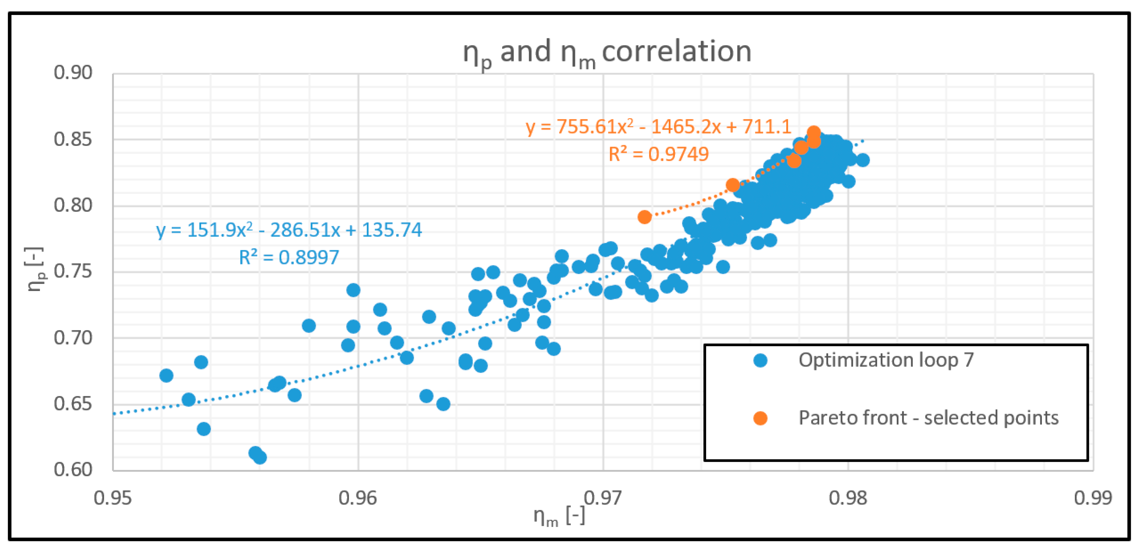
• Relationships between pressure regeneration efficiency and flow inhomogeneity.
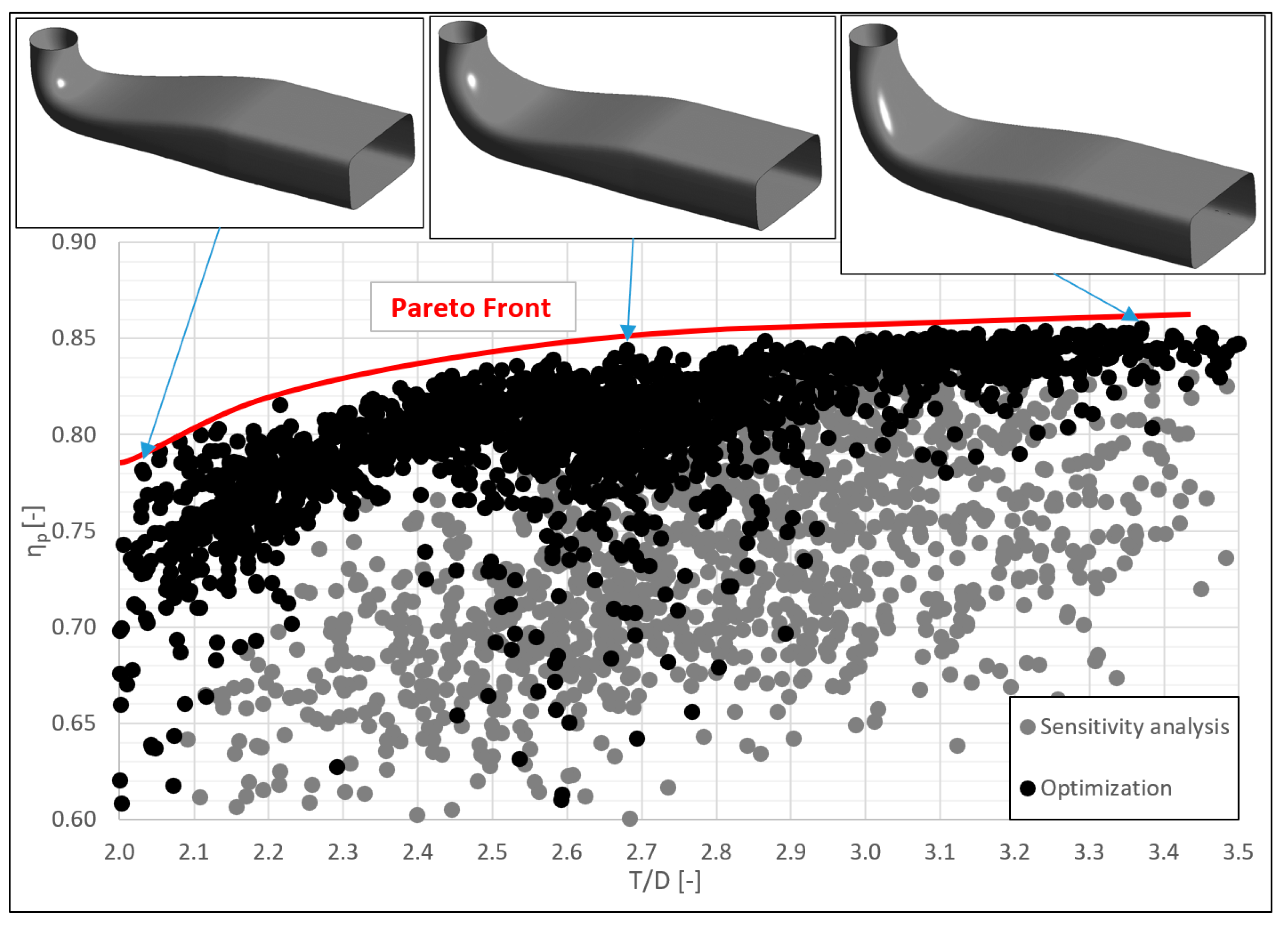
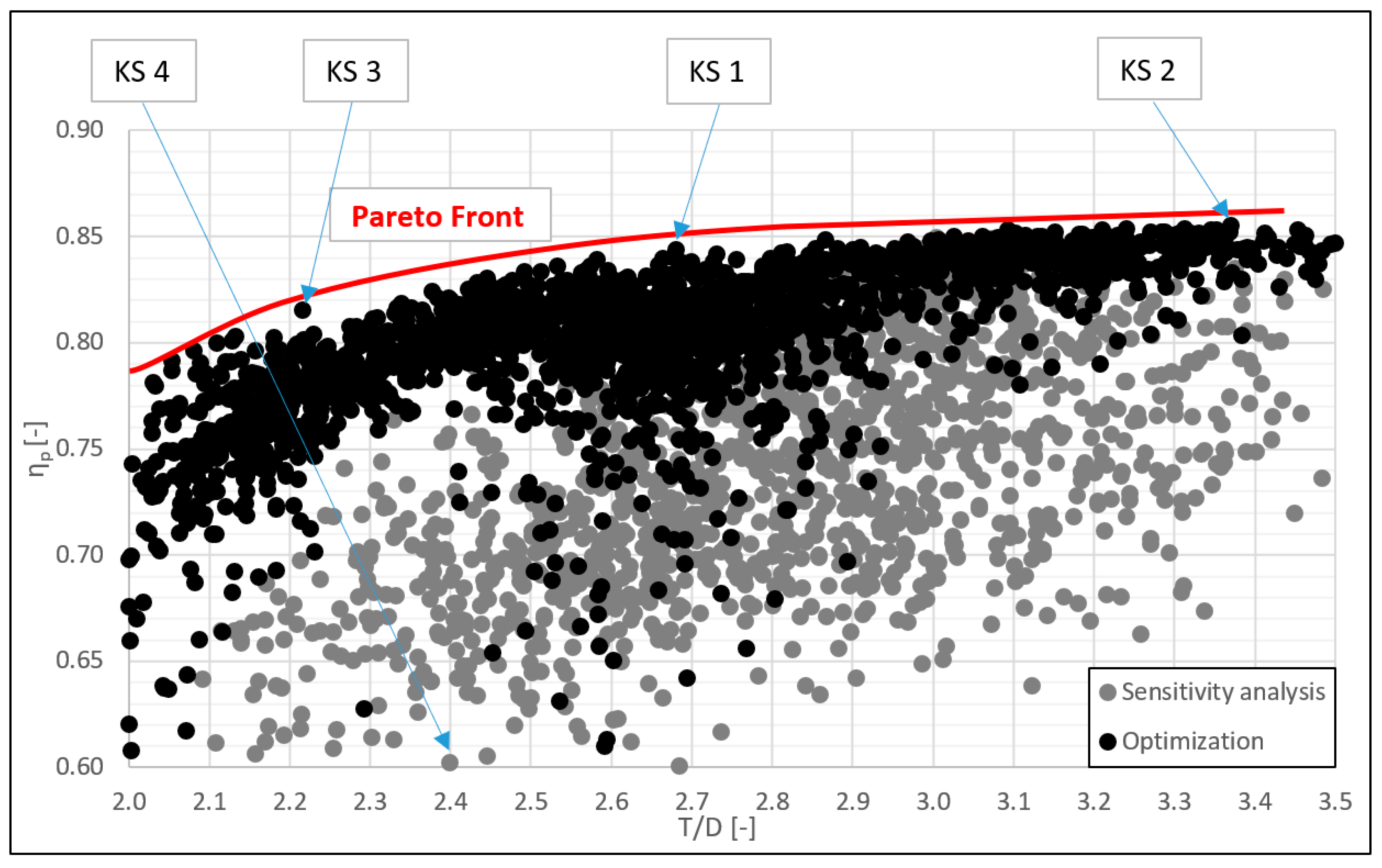
• The resulting set of candidates (Pareto front) with the highest pressure regeneration efficiency and different elbow draft tube heights.
• Performance comparison of the turbine with different elbow draft tubes and with straight draft tube.

The primary objective of this paper is to create a Pareto front of EDT shapes with different construction heights and the highest-pressure regeneration efficiency (further discussed in Section 4.1) using the CFD optimisation methods. This approach enables the selection of EDT for different locations, which is essential because the height of the EDT plays a crucial role in the construction price. The price increases with increasing construction height more than linearly—we expect roughly with the second power.

3. Variable Speed Propeller Specifics

The shape of the velocity field at the inlet of the DT is fundamental for the EDT’s behaviour and optimisation itself. Compared to the classic Kaplan turbine [16], the residual rotation of the variable speed propeller turbine’s velocity field at the exit of the runner is minimal, especially in the range of 80–130% of Q_BEP (Figure 1). Residual rotation can be described by the Swirl number [20]:

$${\mathrm{S}}_{\mathrm{n}}=\frac{\int {\mathrm{v}}_{\mathrm{ax}}\times {\mathrm{v}}_{\tan }\times \mathrm{r} \mathrm{dS}}{\mathrm{R}\times \int {\mathrm{v}}_{\mathrm{ax}}^2 \mathrm{dS}}$$

(1)

where $v_{ax}$ [m/s], $v_{tan}$ [m/s] are the axial and tangential velocities at the inlet profile to DT, r [m] is the radius of the point velocity, and R [m] is the inlet profile radius.

4. Optimisation Process

4.1. Methodology for Draft Tube Assesment

To evaluate the proposed EDT designs, we use two objective functions that are partially contradictory. The first function expresses the rate of kinetic energy recovery of EDT. The second function considers the height of EDT and the associated construction costs.

Usually, the maximization of pressure recovery factor c_p [13] is usually used to assess the efficiency of the conversion of the kinetic energy at the inlet of the DT. Other papers deal with the minimization of hydraulic losses in EDT. A combination of those attitudes is most frequent [11,12]. Our article uses a modified c_p criterion, which we call the pressure regeneration efficiency η_p (Equation (2))—our main output parameter. It evaluates the precise conversion of kinetic energy into pressure, as it is calculated with the actual kinetic energy, including the influence of non-uniformity and not only with the velocity head itself.

$${\mathsf{\eta }}_{\mathrm{p}}=\frac{{\mathrm{c}}_{\mathrm{p}}}{\mathsf{\alpha }}=\frac{{\overline{\mathrm{p}}}_{\mathrm{s};\mathrm{out}}-{\overline{\mathrm{p}}}_{\mathrm{s};\mathrm{in}}}{\mathsf{\alpha }\times \frac{\mathsf{\rho }}{2}\times {(\frac{\mathrm{Q}}{{\mathrm{A}}_{\mathrm{in}}})}^2}$$

(2)

where ${\overline{p}}_{s;in} \left[\mathrm{Pa}\right], {\overline{p}}_{s;out} \left[\mathrm{Pa}\right]$ are the area-averaged values of the static pressure at the inlet or outlet profile of the DT, α [-] coefficient for non-uniformal axial velocity profile [21] (sometimes called Coriolis coefficient [2]), $\mathsf{\rho }$ [kg.m⁻³] is water density (in our case 999.9 kg.m⁻³), Q [m³.s⁻¹] is the volumetric discharge, and A_in [m²] is the cross-section area at the entrance to the DT. Coefficient α is calculated as follows:

$$\mathsf{\alpha }=\frac{{\int }_{\mathrm{A}}{\mathrm{u}}^3\mathrm{dA}}{\overline{{\mathrm{U}}^3}\mathrm{A}}$$

(3)

where $u$ [m.s⁻¹] is the normal component of the point velocity, $\overline{U}$ [m.s⁻¹] is the area-averaged normal velocity, and $A$ [m²] is the cross-sectional area.

The difference between the actual value of the dynamic pressure (kinetic energy) at the DT inlet and the simple velocity head depends on the unevenness of the velocity profile, i.e., the coefficient α. For example, in our case, in the DT inlet for Q_max is equal to 1.12.

Another option for defining the primary objective function is minimizing hydraulic losses [12] (maximizing the “efficiency” of the DT [7]). In our case, we fixed the area of the exit profile. In that case, the values of hydraulic losses and η_p correlate closely, and there is no need for two identical objective functions. However, we evaluated this function, taking into account the energy losses in the draft tube. We call it η_m:

$${\mathsf{\eta }}_{\mathrm{m}}=(1-\left(\frac{{\overline{\mathrm{p}}}_{\mathrm{t};\mathrm{in}}-{\overline{\mathrm{p}}}_{\mathrm{t};\mathrm{out}}}{\mathsf{\rho }\times \mathrm{g}\times \mathrm{H}}\right))$$

(4)

where ${\overline{p}}_{t;in} \left[\mathrm{Pa}\right] a {\overline{p}}_{t;out} \left[\mathrm{Pa}\right]$ is the mean value of the total energy (static + dynamic) on the inlet and outlet profiles of the draft tube, respectively, ρ [kg.m⁻³] is water density, g [m.s⁻²] is the gravitational acceleration (in our case 9.80665 m.s⁻² and H [m] is the net head of the turbine (according to the IEC 62006 standard [22]).

The second output parameter is the construction height T (respectively the ratio of the runner diameter to the construction height T/D), which is defined by the choice of shape parameters of the EDT. F. de Siervo and F. de Leva [23] evaluated the T/D ratio for more than 130 EDTs of classic Kaplan turbines, which ranged from 1.6 to 3.2, with an average of 2.2. Based on their research, they claim that the construction height of the EDT is independent of the specific speed of the turbine. Unfortunately, it is impossible to conclude such an extensive analysis from their research, as we need to determine the exact characteristics of the examined EDTs (such as c_p values).

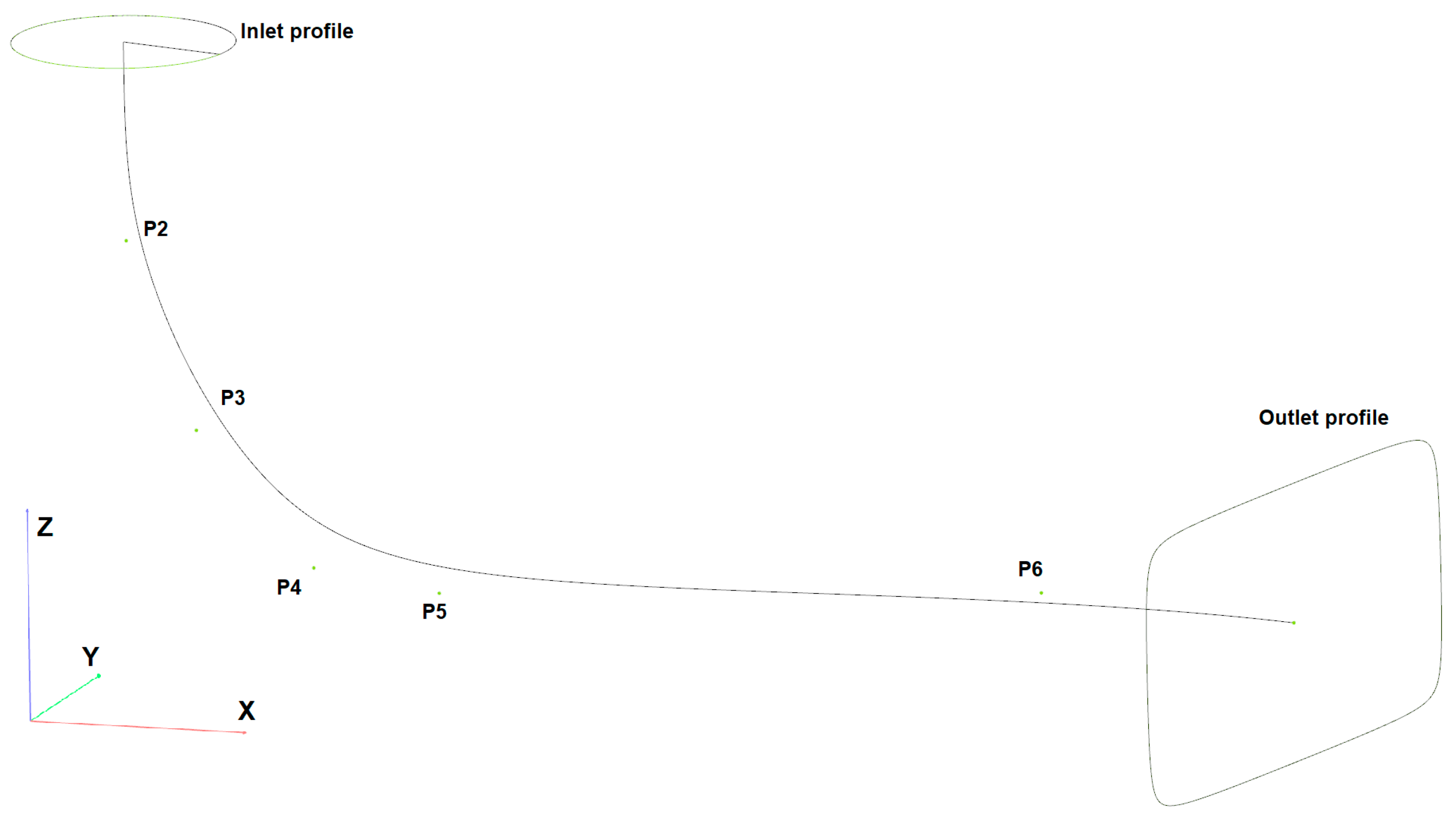
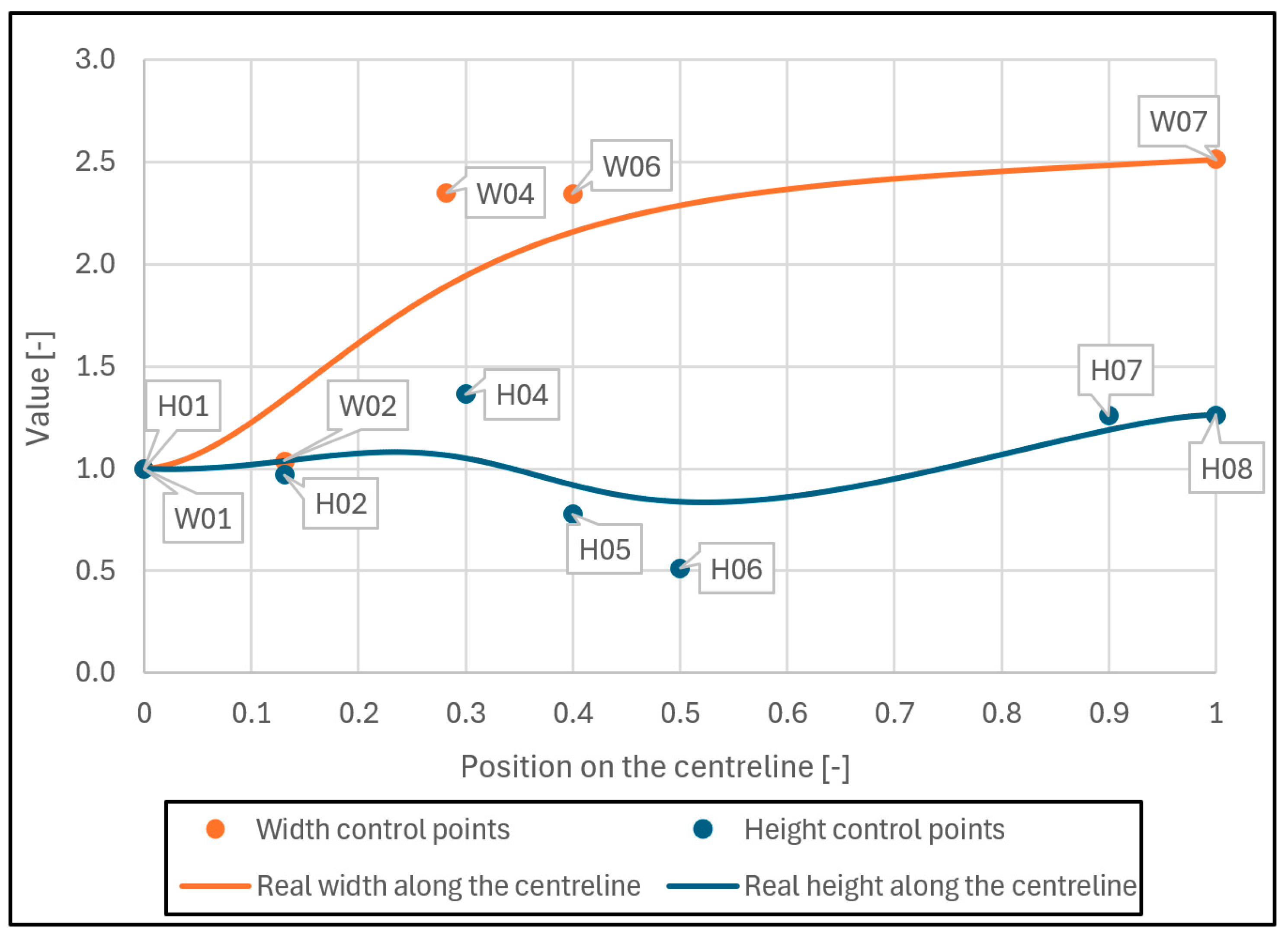
4.2. Geometry Shape Parametrisation

The existing literature does not present any uniform view of the parameterisation of the EDT geometry. For example, Gubin [24] states that there are 20 parameters that can be used to describe EDT. Other authors like Mun et al. [13] or Lyutov et al. [2] describe EDT using 9 independent parameters.

In this study, geometry parametrization was performed in the CAESES 4.2.1 software [25]. In shortcut, our approach is following:

• The fixed inlet profile of EDT (outlet profile of runner chamber)
• The fixed shape of the outlet profile (rectangle with rounded corners; rectangle aspect ratio is 2:1). The position of the outlet profile can change.
• The shape of EDT is defined by the centreline. The height and width change along the length of the centreline.
• The symmetry of EDT—centreline lies in the vertical plane.

The EDT centreline (Figure 2) is defined by seven parameters—points through which the five-degree polynomial spline is fitted. The first point is the centre of the inlet profile and is fixed. The next P2 to P6 have fixed X and Y positions, but their Z coordinate allows to mode and therefore changes the height of the draft tube (see coordinate direction in Figure 2). The last point on the centreline is the centre of the rectangle outlet profile and allows movement in the Z position. After the sensitivity analysis was carried out, the number of parameters was set to 5—named shift in Z direction of P2, P3, P4, P5, and shift of P5 in X direction—overall five parameters describing a centreline. The parameters are bundled together to minimize the invalid shapes of individual EDT shapes.

The cross-section area is defined by changing the height and width along the length of the centreline. The changing of height and width of the cross-section profile along the centreline is defined by a polynomial of the fifth degree, which passes through the points, i.e., the parameters. In Figure 3, there are five parameters defining the width of a cross-section along the centreline. The first and last W01 and W07 parameters are fixed and defined by the inlet and outlet profiles, respectively. There were originally two more parameters (W03 and W05), but these parameters were removed during the first sensitivity analysis. These two parameters contributed minimally to increasing η_p, but they unnecessarily expanded the design space. The remaining parameters sufficiently ensured the shape’s flexibility. Overall, the final parameter η_p was not too sensitive to width changing along the centreline. In the final optimisation, only three width parameters, W02, W04, and W06, were changed. In Figure 3, seven parameters define the cross-section height along the centreline. Again, the first and last parameters are fixed by inlet and outlet profile height. Four parameters, H02, H04, H05, and H06, were allowed to change in the final optimisation. It is worth noting that the position of width and height is related to the normalized value of the centreline length (start is 0, end is 1). Overall, the shape of EDT was defined by twelve parameters (

Table 1. Table of shape parameters minimum and maximum values.

Table of Geometry Parameters	Height Definition				Width Definition			Centreline Definition
	H02	H04	H05	H06	W02	W04	W06	P2_Z	P3_Z	P4_4	P5_Z	P5_X
	[m]	[m]	[m]	[m]	[m]	[m]	[m]	[m]	[m]	[m]	[m]	[m]
Minimum	0.900	0.601	0.500	0.300	0.900	2.000	2.200	0.050	−0.350	−0.400	−0.479	−1.000
Maximum	1.100	1.499	0.900	0.750	1.100	2.500	2.650	0.469	0.200	0.550	−0.051	−1.999

)—five for the definition of centreline, three for width definition, and four for height definition. This setting enabled both the modification of the shape and a significant change in the global height of the EDT and simultaneously retained a reasonable number of parameters.

4.3. Grid Scaling Test

Extensive testing of the grid was performed for the initial shape of the EDT. Grids were created in the ICEM CFD software 2021 R1 [26]. Significant inspiration was taken from sensitivity analysis on EDT grids given by Devals et al. [27]. Concerning the computational complexity, various grids were tested, with the usage of the wall functions (average y+ around 60). The grid testing was performed for the shape of the EDT, which emerged from the first sensitivity analysis (Figure 4). The discretization error estimation using the Grid convergence index (GCI) method described by Celik et al. [28] was used. In the table below (

Table 2. GCI parameters evaluation.

Grid no.1	N1 (mil.)	5.15
Grid no.2	N2 (mil.)	1.07
Grid no.3	N3 (mil.)	0.47
Grid refinement factor 12	r21	1.69
Grid refinement factor 23	r32	1.32
ηp grid no.1	ηp1	80.85%
ηp grid no.2	ηp2	81.92%
ηp grid no.3	ηp3	83.07%
Apparent order	p	1.854
Extrapolated value	η21p ext (-)	80.20%
Approximate relative error	ea21	0.0133
Extrapolated relative error	eext21	0.0080
Grid convergence index grid 1 and 2	GCI21 fine	0.0101
Grid convergence index grid 2 and 3	GCI32 medium	0.0269

), we present computed parameters of the GCI method to evaluate the numerical uncertainties and extrapolated value of η_p. An extrapolated value of η_p equal to 80.20% was calculated for a grid with infinitely small elements. However, to enable effective optimisation, a structured grid with 1.07 million was used for further optimisation. That was a necessary trade-off to speed up the optimisation.

4.4. Numerical Setup

The point with high load (Q_max of our variable speed turbine “Mohelka” with Q₁₁ = 1.99 m³.s⁻¹, n₁₁ = 178 rpm—see Figure 5a was chosen to optimise the EDT. This operating point is very close to the maximum unit power P₁₁ of the turbine.

The steady-state RANS CFD model was calculated in ANSYS CFX [26], an established commercial package with high accuracy and high-quality prediction of the behaviour of the given hydraulic problem. The turbulent k-ω SST model, initially introduced by Menter [29], was used. In these days, this model is by far the most widely used in CFD analysis of turbines and DTs [7,12,13,30]. The “High-resolution” advection scheme [31] was used, which allows automatic switching between the second- and first-order numerical scheme. The upper boundary condition was given as velocities in cylindrical sections [14], turbulence kinetic energy k, and turbulence eddy dissipation ε. Figure 5b explains the shape of the velocity profile used for the optimisation. The lower boundary condition was the average value of the static pressure. The condition of achieving the standard deviation of the monitored η_p at the outlet of the EDT for the last 50 iterations was chosen as a convergence criterion. At the same time, the RMS (root-mean-squared) residuals of pressure, mass momentum, and turbulence parameters were checked if holds were below 10⁻⁴.

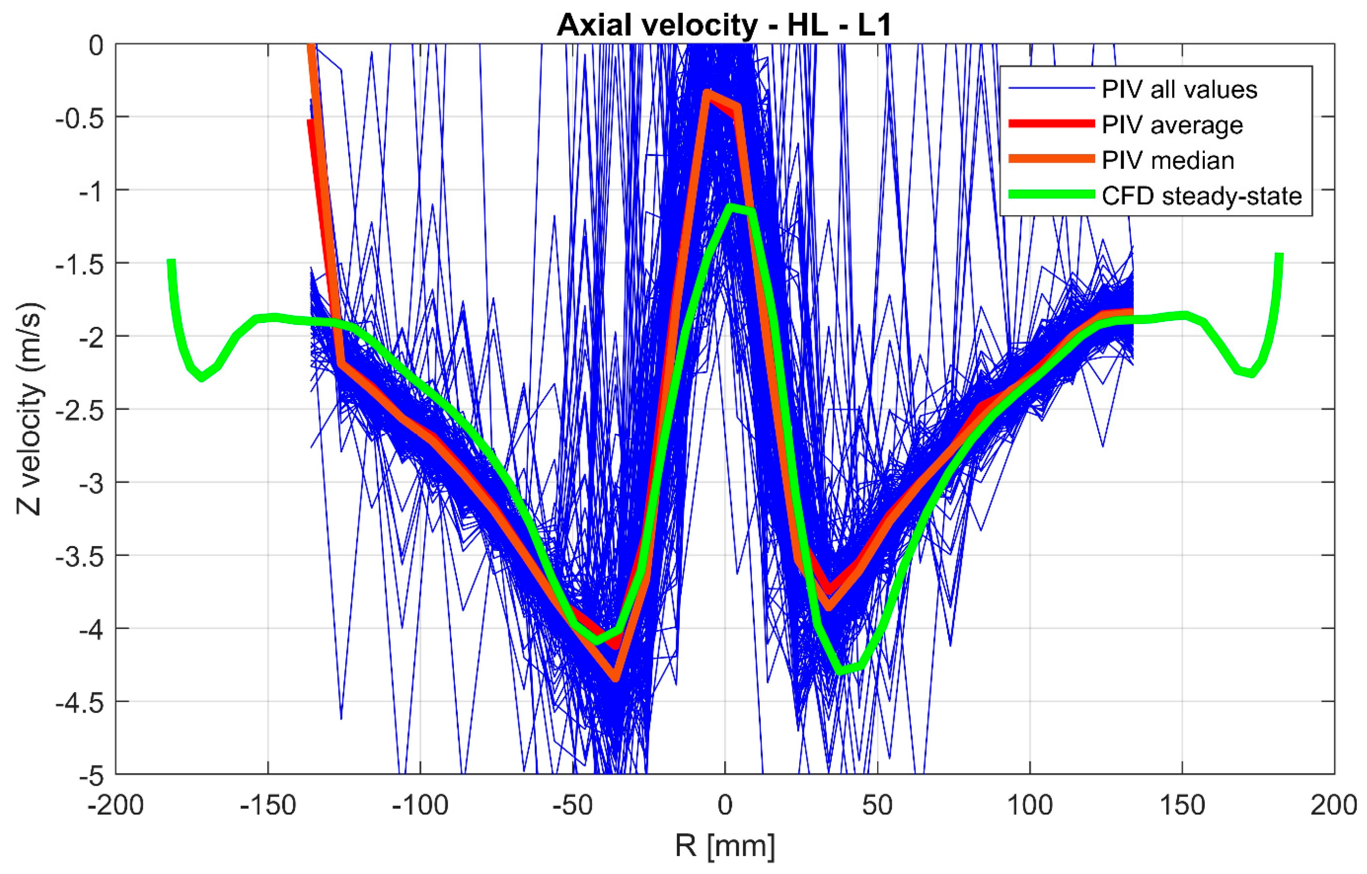
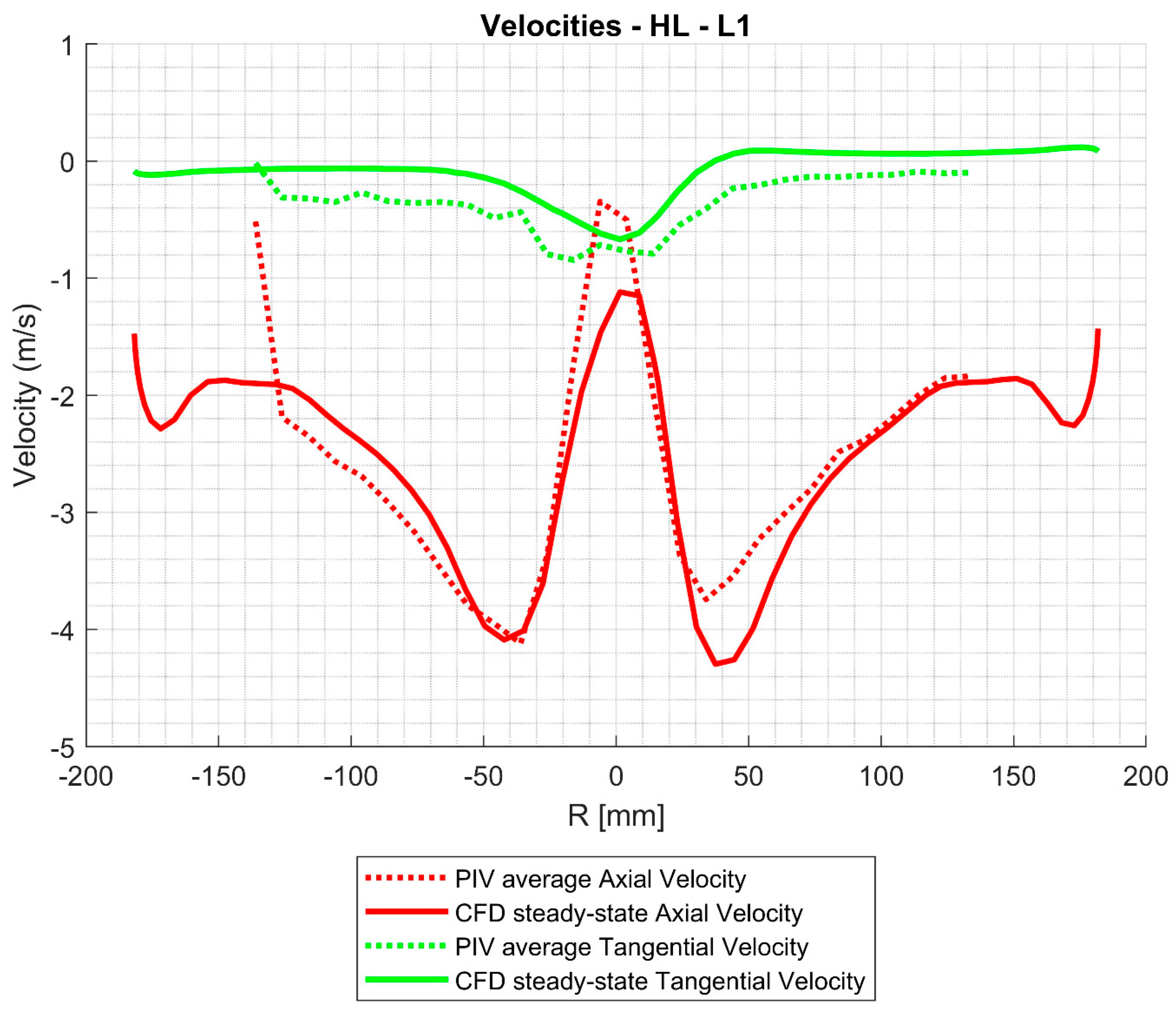
4.5. Validation of Numerical Model

Since it was a design stage, the calculations could not be verified experimentally. However, previous work regarding the same concept of variable speed turbines (Bílková et al. [3]) compared the CFD and measured data of manufactured turbines. Since the measurement was done in situ without complying with the values specified in the standard IEC 62006, the precise error values are unknown. Unfortunately, we could not find open data files for the propeller or at least the Kaplan turbine regarding measuring velocity fields behind the runner. The closest available and reliable data for our optimisation was the Francis 99 project [32]. Grids were taken from the Francis 99 project, and the analysis of numerical settings’ influence on the results was carried out using the same setting for the optimisation of the EDT. The calculations were performed with the use of rotational symmetry. The model overpredicts the efficiency for all calculation points (

Table 3. Comparison of numerical and experimental results of whole turbine unit hydraulic efficiency.

	PL	BEP	HL
	[%]	[%]	[%]
Francis 99	90.1	92.4	91.7
Our CFD sim.	93.6	94.2	93.0
Difference	3.5	1.8	1.3

)—part load (PL), best efficiency point (BEP), and high load (HL), and the numerical model underestimates the losses in the turbine. This fact partially corresponds with the results of Trivedi et al. [31].

We further examined the velocity profiles in profile L1 at the beginning of the EDT (for PIV measurement and other info, see [32]). In Figure 6 can be seen the example of the evaluation of PIV-measured axial velocities (from the Francis 99 website) and numerical ones from our CFD analysis (green line) for high load. Figure 7 compares axial and tangential velocities for averaged PIV values and CFD steady state.

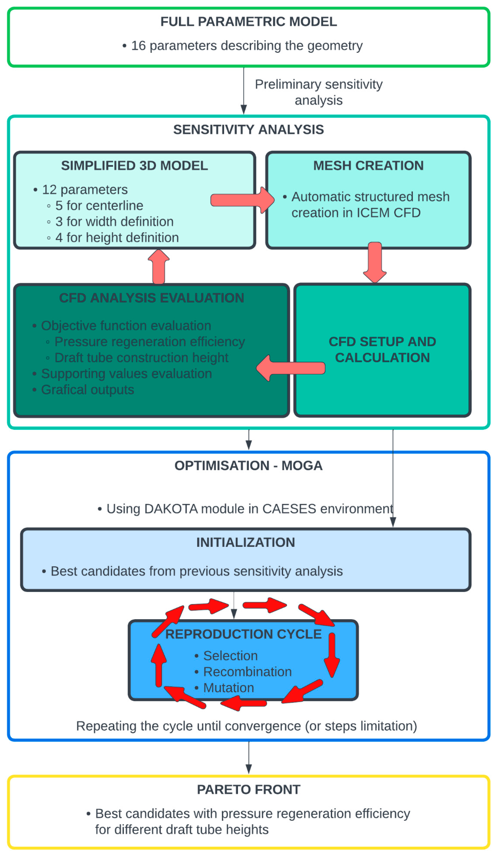
4.6. Sensitivity Analysis and Optimisation

First, a sensitivity analysis was performed for a more extensive range and number of parameters to obtain an initial description of the design space. Two target objective functions are the pressure regeneration efficiency η_p and the ratio of the runner diameter to the elbow draft tube construction height T/D. As previously mentioned, the EDT inlet’s velocity field corresponds to the point of maximum turbine discharge Q_max. This is the point with the highest velocities and the least favourable condition for EDT. The direction and magnitude of the velocity field rotation for our variable speed turbine is similar in the range of about 80–130% Q_BEP (Figure 8). Therefore, the single-point optimisation was performed as we expected that multipoint optimisation would not bring significant benefits. The benefit of the EDT for small discharges is insignificant, especially from the global point of view on energy production.

Tests were performed to eliminate insensitive parameters. Finally, the number of free parameters settled at twelve. The definition of the cross-section utilizes seven free parameters, and the definition of the EDT centreline utilizes five parameters.

After the initial sensitivity analysis, several optimisations using genetic algorithms (MOGA) [33] were performed in the areas with the best η_p and T/D ratios. The procedure was such that we selected the best candidates at the Pareto front from prior sensitivity analysis—the boundary of the best T/D and η_p combinations. These candidates served as starting points for subsequent MOGA optimisations. This procedure proved to be very effective for describing a narrower design space in the selected areas of the construction height T.

The total number of simulations performed was around 4000. For the simulations, the already mentioned high-quality structured grid (approx. 1 million elements) was used, and therefore, the velocity and pressure field in the EDT were sufficiently well described.

5. Optimisation Results

Figure 9 shows all performed simulations. The Pareto front is made up of candidates with the best pressure regeneration efficiency η_p for a given construction draft tube height T/D. It allows a selection of suitable candidates for our type of turbine and any location.

It can be seen from the graph that for EDTs with a considerable height (approx. T/D > 3), there is only a very slight increase in η_p at the cost of a more significant height of the EDT. At the same time, at a low height of the EDT (approx. T/D < 2.2), there is a significant decrease in the efficiency of pressure regeneration η_p.

Improving the EDT characteristics results in an energy production increase that can be roughly calculated as:

$$dP\cong P\times \mathsf{\beta }\times d{\eta }_p \left[\%\right]$$

(5)

where dP [kW] is an increase in the performance of the unit, P [kW] is the original power output of the turbine unit before EDT optimisation, β [%] is the kinetic head ratio [6] (ratio of the kinetic energy leaving the runner on the net head H) and dη_p is an increase in the pressure regeneration efficiency.

For our turbine at the point of Q_max, the kinetic head ratio β equals 32%. On the Pareto front shown in the range T = 2.0 to 3.5, there is a difference in maximal reachable η_p of 7%, which in our case, where with β equals 32%, corresponds to a gain in power output dP of about 2.3%. The Pareto front curve enables the selection of a suitable candidate—it depends on the economic analysis of the price of the construction and excavation works and the benefit of the EDT with higher η_p, respectively, turbine power output.

Figure 10 illustrates the dependence of the pressure regeneration efficiency η_p and the value of the coefficient α in the outlet profile of optimised EDTs. After fitting the points, the coefficient of determination shows a very strong dependence, especially for the chosen shapes on the Pareto front. It can be said, that the more suitable the shape of the EDT, the higher the pressure regeneration efficiency η_p and the more even the velocity distribution in EDT and the outlet profile. These facts are indicated in Lyutov et al. [2].

Below (Figure 11) is presented the correlation η_p and η_m both for one selected optimisation loop and the correlation for several randomly selected draft tube shapes located on the Pareto front. Especially for EDTs located on the Pareto front, the correlation η_p and η_m according to the coefficient of determination R² is very high.

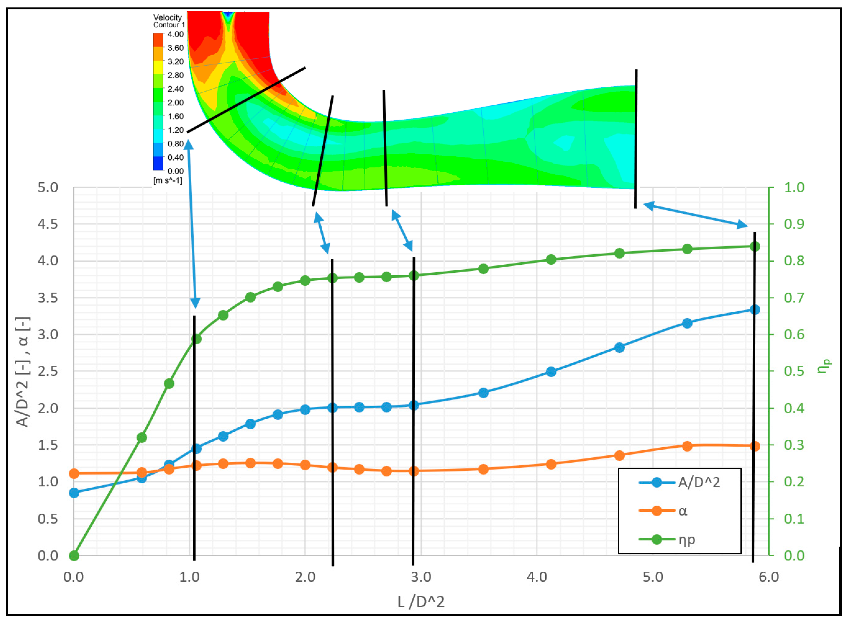
6. Characteristics of Chosen Candidate

For a more detailed analysis, a candidate with a construction height of T/D = 2.68 was selected (further

Table 4. Characteristics of the chosen candidate.

cp	ηp	α	T/D
[%]	[%]	[-]	[-]
94.0	84.1	1.49	2.68

—KS1). This EDT has η_p equal to 84.1%, which corresponds to c_p = 94.0%. This high value is similar to the best results from the literature for the elbow draft tubes of Kaplan turbines (e.g., Orso et al. [12]), moreover, when the ratio of inlet and outlet profile of draft tube A₃/A₄ is only about 0.25 (Orso about 0.20) and at the same time operating our turbine for the Q_max point.

The graph below (Figure 12 and Figure 13) shows the values of the cross-sectional area, the Coriolis number α, and the pressure regeneration efficiency η_p along the centreline length of the selected optimised EDT. Most of the kinetic energy is recovered in about the first third of the length of the EDT. Also, in contrast to some EDTs from the existing literature [14], there is no significant decrease in the cross-section area behind the point of transition to the horizontal direction (between values 2 and 3 of L/D²).

7. Comparison of Different Draft Tubes

Next, Figure 14, we proceeded to compare the selected shapes of draft tubes—previously presented KS1, then high elbow draft tube (KS2), low height draft tube (KS3), and inappropriately shaped KS4.

Concurrently, they were compared with a selected simple conical draft tube (straight draft tube—SDT)-see Figure 15. The SDT shape is defined as follows:

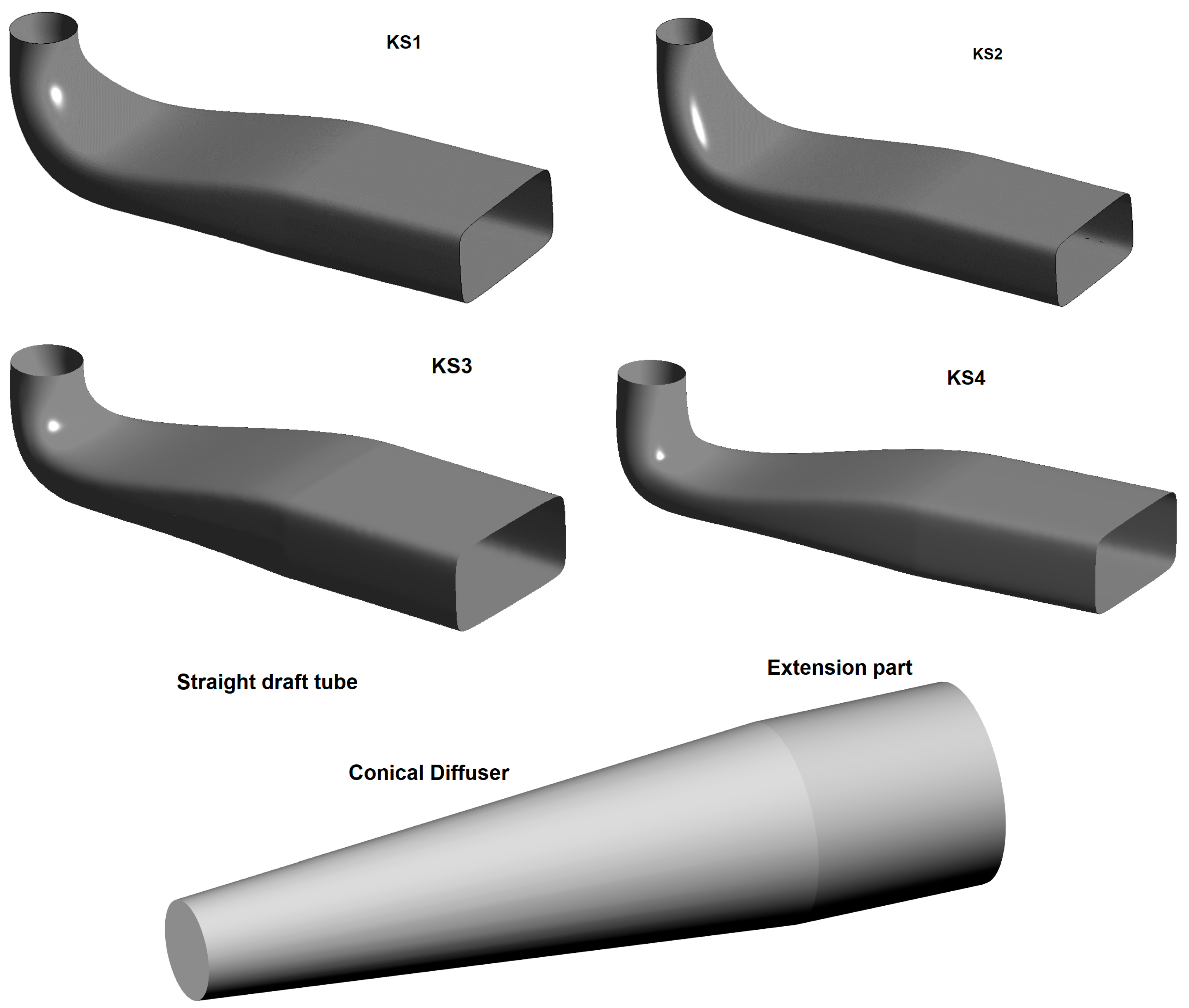
• The area of the output profile of the SDT is identical to KS1.
• The length of the centreline of the SDT is identical to that of the KS1 which results in a half angle θ equal to 4.55°.
• Computational grid is as similar as possible (number of elements and overall characteristics of the grid).
• CFD calculation settings are identical.

The methodology for comparing different draft tube characteristics is as follows:

• After checking the convergence of CFD calculations, export the numerical results of the quantities of interest.
• Processing variables in MATLAB [34].
• Surface fitting of data points with the aim of achieving the highest possible values of the coefficient of determination R². The polynomial fitting method (poly44) was used to fit the surfaces. This will give us 3D surfaces (and contours in 2D) for a more comprehensive display of the machine’s characteristics.
• Creating the ideal coupling of our variable speed turbine—maximum efficiency for individual unit discharges Q₁₁.
• Display or compare the variables of interest in 3D (surfaces), the same in a 2D plan view (contours), and mutually compare the progress for the actual operation of turbines with variable speeds in ideal connections.

In the graphs below (Figure 16a), you can see the comparison of the individual draft tubes for the ideal coupling of our turbine with variable speeds (maximum achievable η_p for each Q₁₁). In the entire discharge regulation range, according to the assumptions, the straight draft tube has the highest efficiency η_p. Elbow draft tubes generally have a lower η_p because there is no change in flow direction in the SDT as in the EDT, which causes additional hydraulic losses in the EDT. Another reason is the flow redistribution from the inlet circular cross-section to the output rectangular one of the EDT. Since the SDT has the same length of the centerline and outlet area as the KS1 EDT, the angle of this SDT is only 4.56° and at this angle, the flow does not break away from the wall, and SDT has a very good pressure regeneration efficiency ηp.

The graph shows the following information for the selected elbow draft tubes:

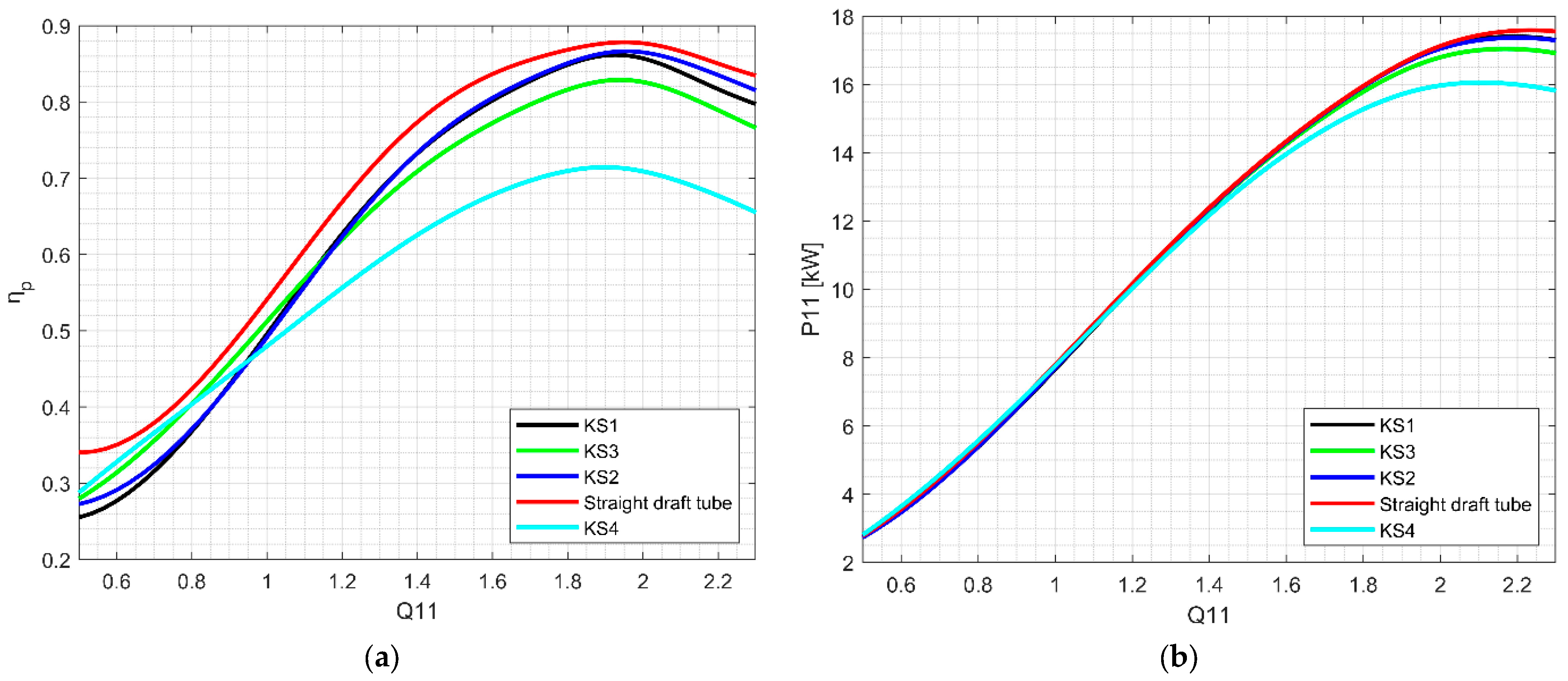
• For large flow rates (Q₁₁ > 2 m³.s⁻¹), the highest draft tube (KS2) has the highest efficiency, followed by the medium height draft tube (KS1), then the elbow draft tube with low height (KS3), and finally the inappropriately shaped draft tube (KS4).
• Surprisingly, for low flow rates (approx. Q₁₁ < 1 m³.s⁻¹), the situation is quite different, and draft tubes with a larger height paradoxically have a lower efficiency of pressure regeneration η_p than elbow draft tubes with a lower height (and even inappropriately shaped elbow draft tube KS4). We believe that the optimisation for one selected point can cause this situation (Q₁₁ approx. 2.0 m³.s⁻¹), and that the numerical model in general is not able to describe the inappropriate flow in these draft tube (especially KS3 and KS4) well enough.

Furthermore, turbines with elbow draft tubes with higher η_p values achieve higher P₁₁, which corresponds to Equation (5). In the case of the draft tubes, there is also a shift in the maximum values of P₁₁ towards higher values of the discharge Q₁₁, which is quite significant from the point of view of achieving a higher discharge capacity of the machine with a suitable shape of the elbow draft tube (Figure 16b).

8. Conclusions and Future Work

Our study presented the extensive optimisation of the elbow draft tube (EDT) for a specific operating point of maximum discharge (Q_max) of variable speed propeller turbine. The specifics of the variable speed turbine and their importance for the optimisation of the EDT were presented, especially the comparison with the standard Kaplan turbine. Furthermore, the methodology for evaluating the characteristics of the intended optimised EDT was presented along with a discussion of other evaluation approaches from the existing literature. We introduced an approach for sensitivity analysis of shape parameterisation and subsequent optimisation using the MOGA algorithm.

Our most notable output, the Pareto front, showcases the best construction height (T/D) and pressure regeneration efficiency (η_p), enabling the selection of an appropriate EDT shape and construction height for various low-head hydropower plant with use of our propeller variable speed turbine. Output analysis revealed a strong correlation between the homogeneity of the velocity field at the EDT outlet profile (α_out) and the pressure regeneration efficiency η_p. An analysis of the hydraulic characteristics of the selected candidate with a T/D ratio equal to 2.68 was also presented. Another output is the performance comparison of different draft tubes (four elbow draft tube from optimisation process and one straight draft tube). The efficiency of the elbow draft tube shapes is very close to the efficiency of the SDT, especially in the area around operating point Q_BEP, indicating very successful EDT shape optimisation.

As for future work, we are currently engaged in more precise validation of our approach, using more advanced turbulence models and advancing the performance of ultra-low-height EDTs. Additionally, we are exploring the feasibility of achieving an optimised smooth EDT design through innovative techniques such as 3D concrete printing, a process that allows for complex geometries and reduces construction time, and precision machining using CNC robotic arms, a method that ensures high accuracy and repeatability. These approaches aim to attain an optimised EDT shape’s desirable and cheap formwork.

References

1. Ko, P.; Matsumoto, K.; Ohtake, N.; Ding, H. Design of a Kaplan turbine for a wide range of operating head—Curved draft tube design and model test verification. IOP Conf. Ser. Earth Environ. Sci. 2016, 49, 10. [Google Scholar] [CrossRef]
2. Lyutov, A. Coupled Multipoint Shape Optimization of Runner and Draft Tube of Hydraulic Turbines. J. Fluids Eng. 2015, 137, 111302. [Google Scholar]
3. Bílková, E.; Souček, J.; Kantor, M.; Kubíček, R.; Nowak, P. Variable-Speed Propeller Turbine for Small Hydropower Applications. Energies 2023, 16, 3811. [Google Scholar] [CrossRef]
4. Kantor, M.; Chalupa, M.; Souček, J.; Bílkova, E.; Nowak, P. Application of genetic algorithm methods for water turbine blade shape optimization. Manuf. Technol. 2020, 20, 453–458. [Google Scholar] [CrossRef]
5. Wilhelm, S.; Balarac, G.; Métais, O.; Ségoufin, C. Analysis of Head Losses in a Turbine Draft Tube by Means of 3D Unsteady Simulations. Flow Turbul. Combust. 2016, 97, 1255–1280. [Google Scholar] [CrossRef]
6. Mosonyi, E. Low-Head Power Plants, 3rd ed.; Akadémiai Kiadó: Budapest, Hungary, 1987; ISBN 963054271. [Google Scholar]
7. Schiffer, J.; Benigni, H.; Jaberg, H. An analysis of the impact of draft tube modifications on the performance of a Kaplan turbine by means of computational fluid dynamics. Proc. Inst. Mech. Eng. Part C J. Mech. Eng. Sci. 2018, 2018, 1937–1952. [Google Scholar] [CrossRef]
8. Pasche, S.; Avellan, F.; Gallaire, F. Part Load Vortex Rope as a Global Unstable Mode. J. Fluids Eng. 2017, 139, 11. [Google Scholar] [CrossRef]
9. Daniels, S.; Rahat, A. Shape optimisation of the sharp-heeled Kaplan draft tube: Performance evaluation using Computotaional Fluid Dynamics. Renew. Energy 2020, 160, 112–116. [Google Scholar] [CrossRef]
10. Favrel, A.; Lee, N.; Irie, T.; Miyagawa, K. Design of Experiments Applied to Francis Turbine Draft Tube to Minimize Pressure Pulsations and Energy Losses in Off-Design Conditions. Energies 2021, 14, 3894. [Google Scholar] [CrossRef]
11. Lučin, I.; Sikirica, A.; Šiško Kuliš, M.; Čarija, Z. Investigation of Efficient Optimization Approach to the Modernization of Francis Turbine Draft Tube Geometry. Mathematics 2022, 10, 4050. [Google Scholar] [CrossRef]
12. Orso, R.; Benini, E.; Minozzo, M.; Bergamin, R.; Magrini, A. Two-Objective Optimization of a Kaplan Turbine Draft Tube Using a Response Surface Methodology. Energies 2020, 13, 4899. [Google Scholar] [CrossRef]
13. Nam, M.; Dechun, B.; Xiangji, Y.; Mingri, J. Design optimization of hydraulic turbine draft tube based on CFD and DOE method. IOP Conf. Ser. Earth Environ. Sci. 2018, 136, 9. [Google Scholar] [CrossRef]
14. McNabb, J.; Devals, C.; Kyriacou, S.; Murry, N.; Mullins, B. CFD based draft tube hydraulic design optimization. IOP Conf. Ser. Earth Environ. Sci. 2014, 22, 012023. [Google Scholar] [CrossRef]
15. Ciocan, T.; Susan-Resiga, R.; Muntean, S. Improving Draft Tube Hydrodynamics over a Wide Operating Range. Proc. Rom. Acad. 2014, 15, 9. [Google Scholar]
16. Štefan, D.; Rudolf, P.; Skoták, A.; Motyčák, L. Energy transformation and flow topology in an elbow draft tube. Appl. Comput. Mech. 2012, 6, 14. [Google Scholar]
17. Marjavaara, D. CFD Driven Optimization of Hydraulic Turbine Draft Tubes Using Surrogate Models. Ph.D. Thesis, Luleå Tekniska Universitet, Luleå, Sweden, 2006. [Google Scholar]
18. Demirel, G.; Acar, E.; Celebioglu, K.; Aradag, S. CFD-driven surrogate-based multi-objective shape optimization of an elbow type draft tube. Int. J. Hydrogen Energy 2017, 42, 17601–17610. [Google Scholar] [CrossRef]
19. Sikirica, A.; Lučin, I.; Alvir, M.; Kranjčević, L.; Čarija, Z. Computationally efficient optimisation of elbow-type draft tube using neural network surrogates. Alex. Eng. J. 2024, 90, 129–152. [Google Scholar] [CrossRef]
20. Susan-Resiga, R.; Dan Ciocan, G.; Anton, I.; Avellan, F. Analysis of the Swirling Flow Downstream a Francis Turbine Runner. J. Fluids Eng. 2006, 128, 177–189. [Google Scholar] [CrossRef]
21. Dauhlhaug, O. A Study of Swirl Flow in Draft Tubes. Master’s Thesis, Norwegian University of Science and Technology, Trondheim, Norway, 1997. [Google Scholar]
22. IEC 62006:2010; Hydraulic Machines—Acceptance Tests of Small Hydroelectric Installation. IEC: Geneva, Switzerland, 2010.
23. De Siervo, F.; de Leva, F. Modern trends in selecting and designing Kaplan turbines. Int. Water Power Dam Constr. 1978, 30, 52–58. [Google Scholar]
24. Gubin, M. Draft Tubes of Hydro-Electric Station; Translated from Russian; Amerind Publishing Co.: New Delhi, India, 1973; ISBN 621.244-225.14. [Google Scholar]
25. CAESES Software. Available online: https://www.caeses.com/ (accessed on 10 August 2023).
26. ANSYS Software. Available online: https://www.ansys.com/ (accessed on 10 August 2023).
27. Devals, C.; Vu, T.; Zhang, Y.; Dompierre, J.; Guibault, F. Mesh convergence study for hydraulic turbine draft-tube. IOP Conf. Ser. Earth Environ. Sci. 2016, 49, 082021. [Google Scholar] [CrossRef]
28. Celik, I.B.; Ghia, U.; Roache, P.J.; Freitas, C.J. Procedure for Estimation and Reporting of Uncertainty Due to Discretization in CFD Applications. J. Fluids Eng. 2008, 130, 4. [Google Scholar] [CrossRef]
29. Menter, F. Two-equation eddy-viscosity turbulence models for engineering applications. AIAA J. 1994, 32, 1598–1605. [Google Scholar] [CrossRef]
30. Fleischli, B.; Del Rio, A.; Casartelli, E.; Mangani, L.; Mullins, B.; Devals, C.; Melot, M. Application of a General Discrete Adjoint Method for Draft Tube Optimization. IOP Conf. Ser. Earth Environ. Sci. 2021, 774, 11. [Google Scholar] [CrossRef]
31. Trivedi, C.; Cervantes, M.; Gandhi, B.; Dahlhaug, O. Experimental and Numerical Studies for a High Head Francis Turbine at Several Operating Points. J. Fluids Eng. 2013, 135, 17. [Google Scholar] [CrossRef]
32. Francis-99: Second Workshop; Norwegian Hydropower Centre: Trondheim, Norway, 2016.
33. Nakamura, K.; Kurosawa, S. Design Optimization of a High Specific Speed Francis Turbine Using Multi-Objective Genetic Algorithm. Int. J. Fluid Mach. Syst. 2009, 2, 102–109. [Google Scholar] [CrossRef]
34. MATLAB Software. Available online: https://www.mathworks.com/ (accessed on 10 August 2023).
Figure 1. Comparison of swirl numbers of Kaplan turbine [16] and variable speed propeller turbine.
Water 16 01457 g001
Figure 2. Inlet and outlet profiles and the definition of the elbow draft tube centreline.
Water 16 01457 g002
Figure 3. Definition of width and height along the centreline.
Water 16 01457 g003
Figure 4. ηp dependency on the type of grid and number of elements.
Water 16 01457 g004
Figure 5. (a) Original variable speed unit hill chart; (b) Velocities in the inlet profile of the elbow draft tube.
Water 16 01457 g005
Figure 6. Axial Velocities in L1 for high load.
Water 16 01457 g006
Figure 7. Axial and tangential velocities in L1 profile and high load.
Water 16 01457 g007
Figure 8. Optimisation workflow.
Water 16 01457 g008
Figure 9. All EDT shapes from sensitivity analysis and subsequent optimisation.
Water 16 01457 g009
Figure 10. Dependency of ηp and αout with miniatures of velocity fields (in EDT outlet profile).
Water 16 01457 g010
Figure 11. Correlation of ηp and ηm functions.
Water 16 01457 g011
Figure 12. Cross-section area A, Coriolis number α and ηp dependency on the length of the centreline.
Water 16 01457 g012
Figure 13. Absolute velocities in axonometric view.
Water 16 01457 g013
Figure 14. Chosen elbow draft tubes for comparison analysis.
Water 16 01457 g014
Figure 15. Selected draft tube shapes for comparison.
Water 16 01457 g015
Figure 16. (a) ηp comparison for different draft tubes and (b) P11 comparison of ideal coupling of variable-speed propeller turbines.
Water 16 01457 g016