Article

Enhancing Oil–Water Flow Prediction in Heterogeneous Porous Media Using Machine Learning

1
Civil Engineering School, Qingdao University of Technology, Qingdao 266520, China
2
CNOOC EnerTech-Drilling & Production Co., Tianjin 300452, China
3
School of Petroleum Engineering, China University of Petroleum (East China), Qingdao 266580, China
4
State Key Laboratory of Offshore Oil Exploitation, Beijing 100028, China
5
CNOOC Research Institute Ltd., Beijing 100028, China
*
Author to whom correspondence should be addressed.
Water 2024, 16(10), 1411; https://doi.org/10.3390/w16101411
Submission received: 13 April 2024 / Revised: 7 May 2024 / Accepted: 9 May 2024 / Published: 16 May 2024

Abstract

:
The rapid and accurate forecasting of two-phase flow in porous media is a critical challenge in oil field development, exerting a substantial impact on optimization and decision-making processes. Although the Convolutional Long Short-Term Memory (ConvLSTM) network effectively captures spatiotemporal dynamics, its generalization in predicting complex engineering problems remains limited. Similarly, although the Fourier Neural Operator (FNO) demonstrates adeptness at learning operators for solving partial differential equations (PDEs), it struggles with three-dimensional, long-term prediction. In response to these limitations, we introduce an innovative hybrid model, the Convolutional Long Short-Term Memory-Fourier Neural Operator (CL-FNO), specifically designed for the long-term prediction of three-dimensional two-phase flows. This model integrates a 3D convolutional encoder–decoder structure to extract and generate hierarchical spatial features of the flow fields. It incorporates physical constraints to enhance the model’s forecasts with robustness through the infusion of prior knowledge. Additionally, a temporal function, constructed using gated memory-forgetting mechanisms, augments the model’s capacity to analyze time series data. The efficacy and practicality of the CL-FNO model are validated using a synthetic three-dimensional case study and application to an actual reservoir model.

1. Introduction

Machine learning, encompassing deep learning, has experienced rapid development in various fields such as computer vision and natural language processing by leveraging the power of large-scale datasets [1,2]. The recent emergence of the large language model (LLM), which can generate realistic dialogues, is triggering another surge in artificial intelligence technologies. The application of machine learning involves the utilization of data for feature extraction and analysis where the neural network (NN) serves as a crucial method for learning from data and constructing efficient predictive surrogate models [3].
In reservoir engineering, numerical simulation employs the finite volume method to obtain approximate solutions for PDEs and to forecast the future dynamics of the reservoir. However, numerical methods entail repeated iterative calculations, which incur high computational costs. To address this problem, NNs, as highly potent universal approximators, have been employed to accelerate the forecast process. For example, it is employed to enhance the efficiency of certain steps in the numerical solving procedure in the non-direct approach [4].
There are also methods directly employing neural networks to approximate or solve PDEs. Zha et al. [5] classified PDE-related NNs into three categories: Category 1 is the data-driven method, in which the laws of PDEs are learned using data obtained from numerical simulations, with the model lacking physical significance; Category 2 is the physics-driven method, where NNs are directly trained based on physical laws or equations. They are distinguished by their prominent feature of data-free learning; and Category 3 pertains to methods of physical constraints, wherein physical criteria are embedded within the NN and the resulting NN possesses interpretable physical significance.
For Category 1, Zhu and Zabaras [6] were the first to employ a fully convolutional network (FCN) for flow field prediction of oil reservoirs. They constructed an NN to map the permeability field to the pressure field and the oil saturation field. Ma et al. [7] employed a bidirectional long short-term memory neural network for horizontal stress prediction, effectively capturing the relationship between logging parameters and in situ stress. Tang et al. [8] introduced the ConvLSTM for the prediction of the flow field in a riverine phase reservoir, with the combination of spatial and temporal information prompting favorable results in long-term prediction. Tang et al. [9] also extended the ConvLSTM to 3D flow field prediction with the introduction of the 3D convolution operation. The main shortages of the purely data-driven method are the requirement of massive amounts of data and insufficient model generalization. An adequate solution is the consideration of physical knowledge to increase interpretability. In Category 2, Raissi et al. [10] proposed the currently widely utilized Physics-Informed Neural Network (PINN). At the onset of the training, the governing equations, initial conditions, and boundary conditions are defined, and the network learns the solution by employing the PDE residual in the loss function. This approach has been demonstrated with applicability to both direct and inverse problems. In Category 3, Li et al. [11] introduced the FNO, a method designed for neural networks based on Green’s function, and the Fast Fourier Transform (FFT) for analytics. After training, the network acquires intrinsic physical significance. This approach significantly accelerates the training speed of NNs and enhances the generalization ability.
In actual reservoir simulations, it is imperative to contemplate more intricate scenarios, and methods related to physical significance have been further refined with specific engineering backgrounds. Zhu and Zabaras [6] proposed an unsupervised NN based on physical constraint to achieve efficient prediction and uncertainty quantification of high-dimensional reservoir models. Wang and Zhang [12] proposed a theoretically guided NN for the inverse problem of oil–water two-phase flow in a porous medium. The integration of NNs with the physical background can enhance the efficiency of real-time decision-making [13,14,15]. However, current physical-informed methods still fall short in long-term two-phase flow prediction of actual 3D reservoirs.
In this paper, we propose the CL-FNO, which integrates the Fourier neural operator and the convolutional long short-term memory within a U-shaped encoder–decoder configuration. The FNO module enhances the model’s generalization capabilities by incorporating physical principles, while the ConvLSTM module equips the network with the ability to handle spatiotemporal data. Moreover, the U-shaped architecture effectively unifies multilevel blocks in the network, enabling simultaneous consideration of spatial and temporal information. The new architecture provides an effective way for establishing a practical reservoir prediction surrogate model with complex engineering backgrounds. In Section 2, we delineate the characteristics of some prevalent PDE-learning methods and introduce details of the CL-FNO architecture. In Section 3, the train and test results of the CL-FNO are presented and discussed.

2. Methodology

2.1. Governing Equations of Two-Phase Flow in a Heterogeneous Porous Medium

The expression of the mass conservation equation of the oil and water two-phase flow system is as follows:
· ρ j v j q j l = t ϕ ρ j S j , j = o , w
where j denotes different phases, including oil and water, o is the oil phase and w is the water phase; ρ j is the density; v j is the Darcy velocity; q j l is the source/sink term (the superscript l denotes the cell of the injection/production well); S j is the saturation, and t is time. The Darcy velocity equation is as follows:
v j = K k r j S j μ j p ρ j g z , j = o , w
where k r j is the relative permeability; K denotes the absolute permeability; μ j is the viscosity; g is the gravity acceleration; and z is the depth, m. In the 3D case, the effect on gravity is considered using the following Equation (3):
p i + 1 l = p i l + ρ g Δ z i , j + 1
where i denotes the i-th longitudinal layer. Introducing Equations (2) and (3) into (1) makes the sum of oil and water phase saturations in each cell 1. The pressure difference between the two phases is defined as the capillary pressure, and the initial and boundary conditions, which can be discretized using FVM, are added and the numerical solution can then be obtained using the iterative method.

2.2. Reference Methods

This section provides a detailed exposition of existing PDE-related methods for flow field prediction, primarily encompassing FCN, data-driven ConvLSTM, and PINN FNO with physical significance.
FCN simplifies the solution of PDEs as an end-to-end mapping that can be regarded as a finite-dimensional operator. In practical applications, the neural network is treated as a universal image regression model processing mapping from flow field to flow field. The distinct characteristics of FCN are the utilization of convolution layers without any fully connected layer and the incorporation of dense connections originating from DenseNet [16]. Each convolution layer is cascaded to all preceding layers to facilitate feature reuse and to reduce the gradient vanishing, as depicted in Equation (4).
x l = H x 0 , x 1 , , x l 1
where x l is the input of the l-th layer and H denotes the nonlinear transformation. Zhang et al. [13] applied FCN to the learning of the oil–water two-phase flow, achieving satisfactory results from a high-quality database. However, the over-simplification of the underlying physical principles reduces the generalization of FCN when it is faced with unfamiliar situations.
By considering the role of time, long short-term memory (LSTM) employs a recurrent network architecture that can capture long-term dependency using gate structures [17]. Its general form is represented as follows:
i t = σ W xi x t + W hi h t 1 + W ci c t 1 + b i
f t = σ W xf x t + W hf h t 1 + W cf c t 1 + b f
c t = f t c t 1 + i t tanh W xc x t + W hc h t 1 + b c
where it is the input gate; Wxi, Whi, and Wci are weight matrixes of input data xt, hidden state ht−1 at time t − 1 and cell state ct-1 at time t-1, and bi is the bias of the input gate; ft is the forget gate; Wxf, Whf, Wcf are weight matrixes of input data, hidden state, and cell state; bf is the bias of the input gate; ct and ct−1 are the cell state at time t and t – 1; Wxc and Whc are weight matrixes of input data and hidden state; bc is the bias of the cell state; σ is the Sigmoid activation function; and tanh is the Tanh activation function. The input gate is employed to regulate the memory quantity stored in the cell state, ct, at the current time step. The forget gate, ft, governs the extent of forgetting historical information in the hidden unit, ct. LSTM has been proven to exhibit persistent, adaptive memory and forgetting ability to prevent the issue of vanishing gradients or exploding gradients [18]. However, the basic LSTM is difficult to deal with in the spatio-temporal scenario.
ConvLSTM employs convolutional operations for spatial information extraction to reduce the redundant computation of fully connected layers, enabling the handling of spatial information. The general form of ConvLSTM is represented as follows:
i t = σ W xi x t + W hi h t 1 + W ci c t 1 + b i
f t = σ W xf x t + W hf h t 1 + W cf c t 1 + b f
c t = f t c t 1 + i t tanh W xc x t + W hc h t 1 + b c
where is the convolution operator and is the Hadamard product. Except for the dimensionality of the data, the meanings of the symbolic letters are the same as explained in the previous LSTM formulas. ConvLSTM has been proven to have good accuracy in the flow field prediction of actual 3D reservoirs [19]. However, due to the lack of consideration of the specific details of the prior physics problem, ConvLSTM still has shortcomings in the training process, solution accuracy, and generalization ability.
PINNs incorporate the residual of PDEs, along with initial and boundary conditions, into the loss function for training, thereby achieving data-free learning [10]. The definition of the loss function is shown by Equations (11) and (12). When solving different PDE-related problems, there are various forms of targeted improvements for the PINN-based methods [20,21,22].
L o s s = λ 1 M S E data + λ 2 M S E P D E + λ 3 M S E I C + λ 4 M S E B C
M S E d a t a = 1 N i = 1 N u ^ i u i 2
where MSEdata is the L2 loss of prediction value and the true value, ui is the true value of the i-th g r i d , u i ^ is the NN prediction value of the i-th g r i d , N is the number of mesh grids, MSEPDE is the L2 loss of PDEs residual, MSEIC is the L2 loss of initial condition, MSEBC is the L2 loss of boundary condition, and λ1, λ2, λ3, λ4 are hyperparameters used to balance different loss values. PINNs are capable of data-free training; however, with the increasing complexity of the physical background, the difficulty of training neural networks increases rapidly. In reservoir engineering, the PINN method is also used to predict the underground two-phase flow [12], but the speed is too slow to apply to actual issues.
The FNO stands out as a potent methodology for approximating a sequence of PDEs. Within this framework, the solution operator, denoted as G , acts as a functional mapping, whereby G a = u ; here, a represents the input function and u is the corresponding solution function. The FNO introduces a neural network-based approximation of this operator, designated as G . Consequently, the original mapping process is effectively substituted by G a = u , where G directly estimates the operator G . The learned neural network is theoretically a mapping from infinite dimensions to infinite dimensions. The mapping process of the FNO is presented in Equations (13)–(15):
v 0 x = P a x
v t + 1 x = σ W v t x + K a ; ϕ v t x
u x = Q v T x + q
K ϕ v t x = F 1 R ϕ · F v t x
where x is the coordinate or the sampling position; a is the input function; P is the encoder layers; v t is the output of different layers, t = 0, 1, 2, … T − 1, where v 0 is the encoded a and the others are the output of Fourier layers; T is the total number of Fourier layers; W is the mapping of v t ; K is the kernel function that is used to approximate the integral operator; ϕ is the parameter of the kernel function; Q is the decoding layer; and q is the bias. To improve computational efficiency and take full advantage of the power of the neural network, the kernel function is further simplified to Equation (16) [11].
The FVM and PINN methods usually find the solution u U of the equation directly. The finite-dimension data-driven method is essentially a process of mapping limited quantities of input parameters a A = D ; R d a to the solutions u U = D ; R d u , G : A × Θ U ., although it cannot solve the same kind of PDE problem when the parameter coefficient a A changes. Therefore, the computational costs of both are usually high. FNO adds physical constraints to neural networks, which greatly improves the generalization ability of the model. In FNO research, there is a prediction method that processes the prediction of the neural network into a time series using a sliding time window.
However, for the complex 3D, two-phase, and long-term prediction in an actual heterogeneous reservoir with multiple injection and production wells, the FNO still has shortcomings, including training difficulty and prediction accuracy. This may be due to insufficient utilization of pre-existing spatial structures and temporal sequence information. Therefore, in the following section, our model will be established based on these considerations.

2.3. Convolutional Long Short-Term Memory-Fourier Neural Operator

The original FNO is used for the 2D single-phase flow problem [11]. When extending the architecture-based 3D two-phase problems, the accuracy of the model will decrease due to the inherent regularization effect (or feature loss) during model extraction, particularly the loss of 3D information. We combine the 3D convolution operator and the FNO in parallel, as shown in Figure 1, and Equation (14) is modified to Equation (17):
v t + 1 ( x ) = σ W v t ( x ) + C o n v 3 D v t ( x ) + K ( a ; ϕ ) v t ( x )
where Conv3D is the 3D convolutional operator corresponding to a 3D convolutional block in the NN. Compared with 2D convolution, 3D convolution can extract additional information on channel dimension, corresponding to the engineering problem of the 3D reservoir model, so that the 3D convolution can better learn the longitudinal flow characteristics between layers.
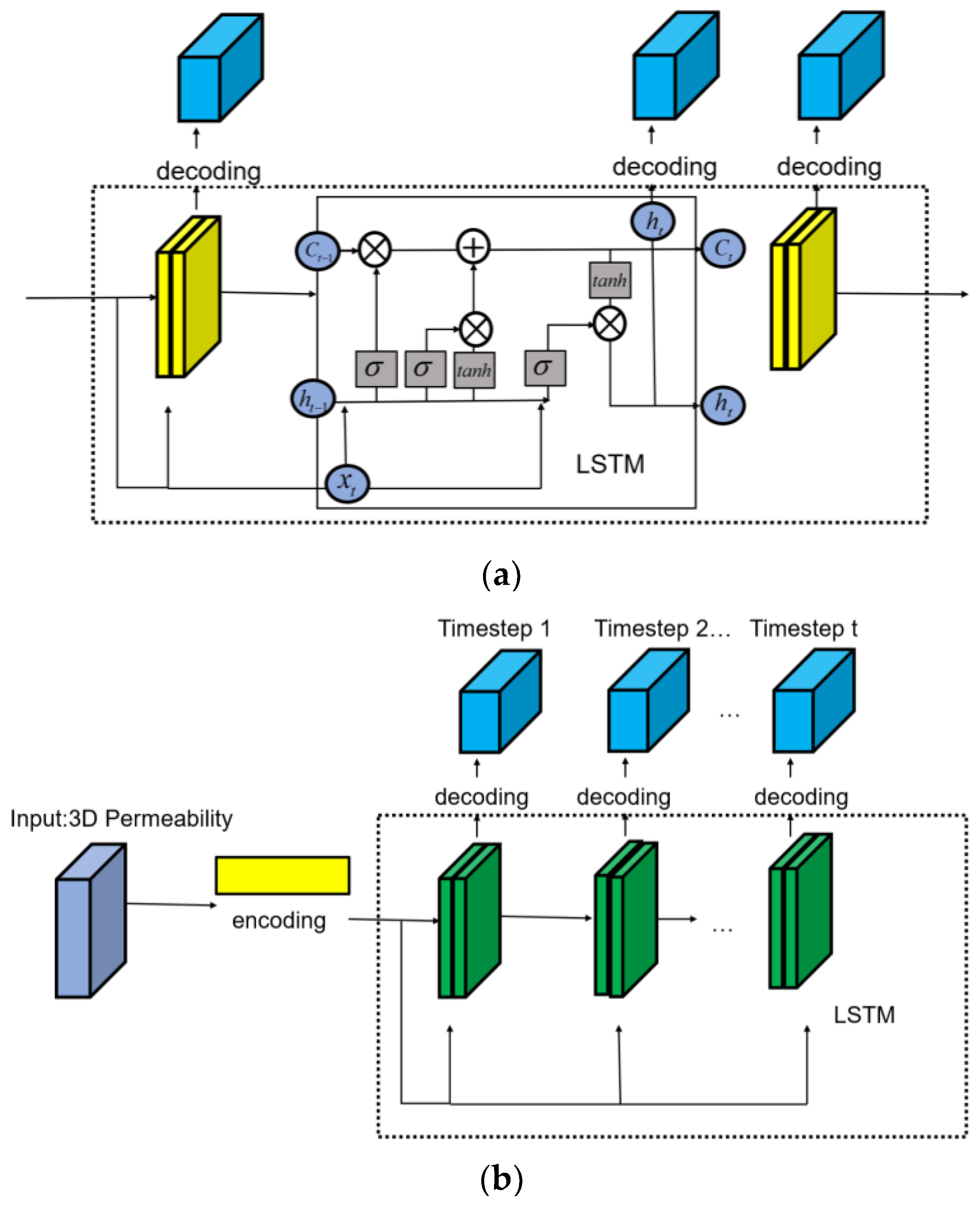
In previous research, when processing time series data with FNO, the network had no memory-forgetting functions, which led to error accumulation in long-term prediction caused by inherent sample bias. To solve this problem, we address the long-term dependencies within the data structure by embedding ConvLSTM modules. The details of ConvLSTM are presented in Figure 2. In particular, we replace the convolution block of the original ConvLSTM with 3D convolution [23], as shown in Figure 2a. Training on time series data follows a technique similar to the one proposed by Li et al. [11]. A notable distinction is that each input batch in our method contains data from a single time step, rather than multiple time steps from a series. This approach deviates from the original FNO and presents challenges for efficient training; nevertheless, by incorporating a temporal function, we successfully address this issue. The predictions are generated incrementally, step by step. The losses from all steps are then averaged and employed to train the network, as illustrated in Figure 2b.
The proposed CL-FNO is presented in Figure 3. The network is mainly composed of the encoding part (including four encoding layers that gradually increase the receptive field of the convolution block), the intermediate part (including four additional physical constraint layers and a memory layer), and the decoding part (including four deconvolution layers that gradually merge hierarchical details). The overall U-shaped structure employs the same skip connection with the U-net between the same level to compensate for feature loss during multiple down samplings. The detailed network information and the data size at/after different levels are shown in Table 1. It should be noted that n in the input 40 × 40 × 20 × n is the number of variables; the number 20 in the last dimension of “intermediate layer 2” is the accumulated result of recurrent decoding part in multiple time steps.

3. Case Study

3.1. Synthetic Case

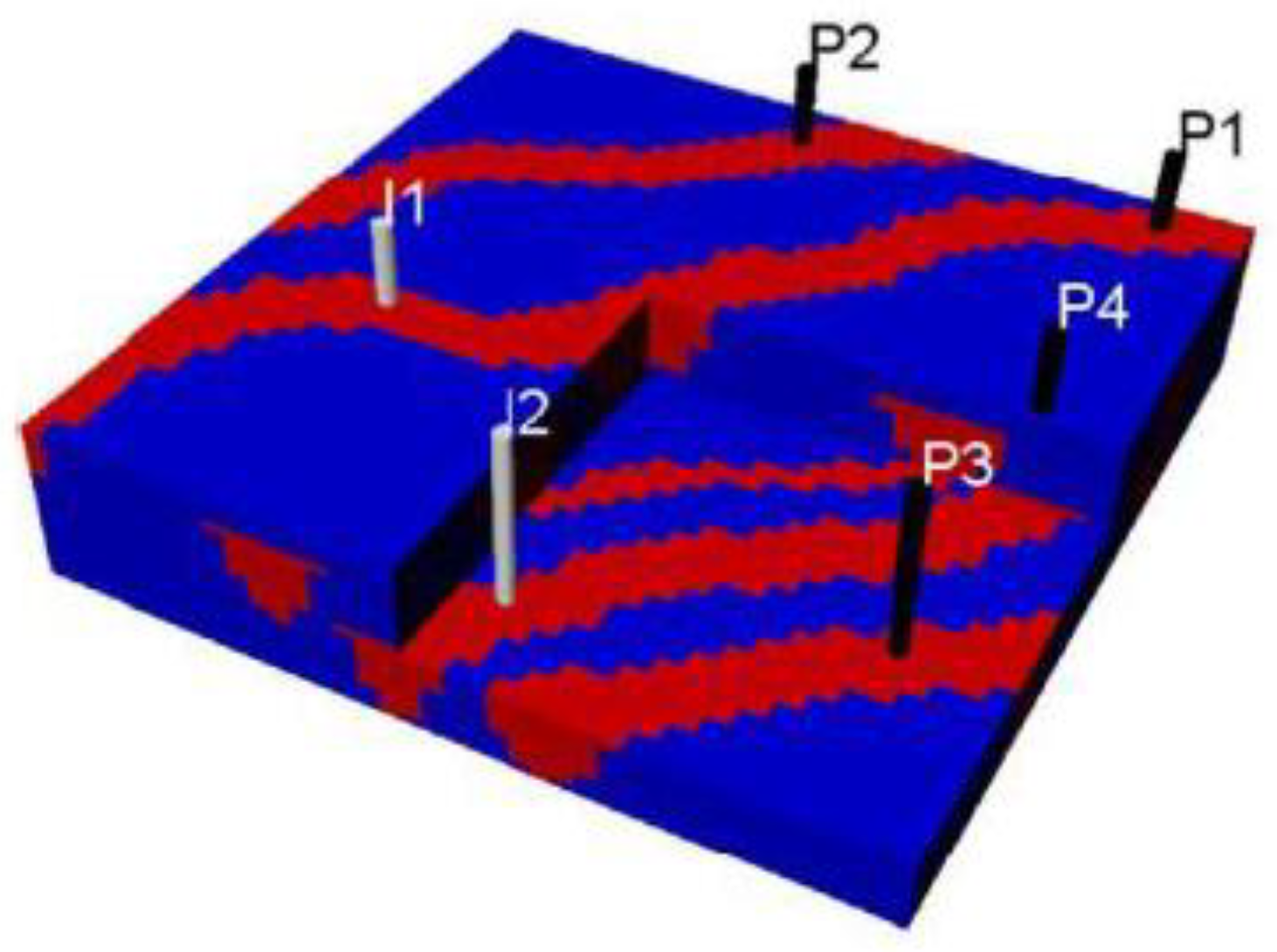
We used a synthetic model to test the effect of CL-FNO on model training and future dynamic predictions. The input of the model is the permeability field, and the output is the pressure and saturation field. The referenced parameter settings are derived from a cut-off portion of an actual reservoir. The synthetic model size is 40 × 40 × 20, with 20 layers in the longitudinal direction. The grid size is 20 m × 20 m × 20 m. Two injection wells (J1, J2) and four production wells (P1, P2, P3, P4) are set in the block. J1, P1, and P2 perforate the upper ten layers, and the other wells perforate the bottom ten layers, as shown in Figure 4. Well control follows the original setting with a target injection and production rate. A total of 2000 3D permeability fields are synthetically generated using a sequential Gaussian method [24]. ECLIPSE software (version 2011.1) was used to generate data for 60 days per time step and 20 time steps per permeability field. Finally, 1600 samples were randomly selected as the training set and the remaining 400 samples were used as the test set.
The size of the input matrix is N , V a r x , V a r y , V a r z , n . N is the batch size; Varx, Vary, and Varz are the resolutions of the 3D data; n are variables number equal to 7, corresponding to rock permeability, 3D location number, initial conditions, and relative permeability, represented as K , x , y , z , q c o n d , k r o , k r w . However, in practice, we found that the training efficiency was too low and the input of relative permeability did not have much effect on improving accuracy. Therefore, we modified the input to { K , x , y , z , q c o n d } . The size of the output matrix is N , V a r x , V a r y , V a r z , T . T corresponds to the accumulated multiple time steps. In our experiment, we employed distinct decoding networks for pressure and saturation, and the overarching training and output process utilized a hard parameter-sharing multitask learning process, thus T is twice the number of model time steps. For all test samples, we calculated the relative root mean square error (RMSE) between the predicted solution of FNO and the solution of the numerical simulation.
R M S E = 1 n i n | y ^ i y i | 2 2
where y i ^ is the prediction value, y i is the true value, and n is the number of observations. To better see the overall error of the output flow fields, we calculated the overall mean relative error (MRE):
δ S = 1 n test   n M n t i = 1 n test   m = 1 n M t = 1 n t S ^ w i , m t S w i , m t S w i , m t
δ p = 1 n test   n M n t i = 1 n test   m = 1 n M t = 1 n t p ^ i , m t p i , m t p i ,   max   t p i ,   min   t
where δ S is the relative error of the saturation field; δ p is the relative error of the pressure field; n test is the total number of test samples; n M is the total number of grids; nt is the number of time steps; S ^ w i , m t is the prediction saturation; S w i , m t is the true saturation; p ^ i , m t is the prediction pressure; p i , m t is the true pressure; p i ,   max   t is the maximum pressure; and p i ,   min   t is the minimum pressure.
Based on the PyTorch framework, Adam is used for training, the initial learning rate is set to 0.001, the weight decay is 0.0005, the batch size is set to 20, the L2 loss function is calculated for backpropagation, and other parameters are kept at default Settings. The training is performed on NVIDIA K80 GPU (24G). Specifically, in the Fourier block, the number of low-frequency modes, s, is set to 12. The above settings are the recommended choices obtained through multiple experiments during our study and will also be used in the next application case. Other details of training processes are the same as those of previous works [14]. The network structure of 3D ConvLSTM is the same as that described in previous research [19], in which the convolution size is adaptively adjusted to maintain the input and output sizes in this paper, while the time series data structure, hyperparameter settings, and training process are the same as those of the CL-FNO in this paper. An automated program was prepared to complete the training of NNs for 100 epochs.
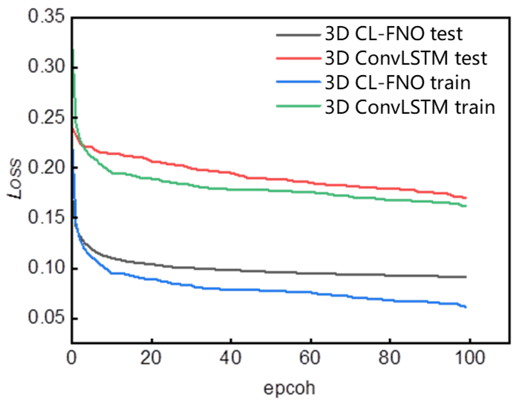
In Figure 5, it can be seen that the loss of CL-FNO reduces quickly, corresponding to higher accuracy. At 100 epochs, the loss of ConvLSTM still decreases, but at a very slow speed, which indicates an actual slower training speed. ConvLSTM is considered a SOTA module for spatiotemporal information prediction widely used in various spatiotemporal information processing, but it still lacks consideration of the physical background. With the addition of physical constraints, CL-FNO has a clear first principles background instead of a black box, which significantly improves the performance of the model.
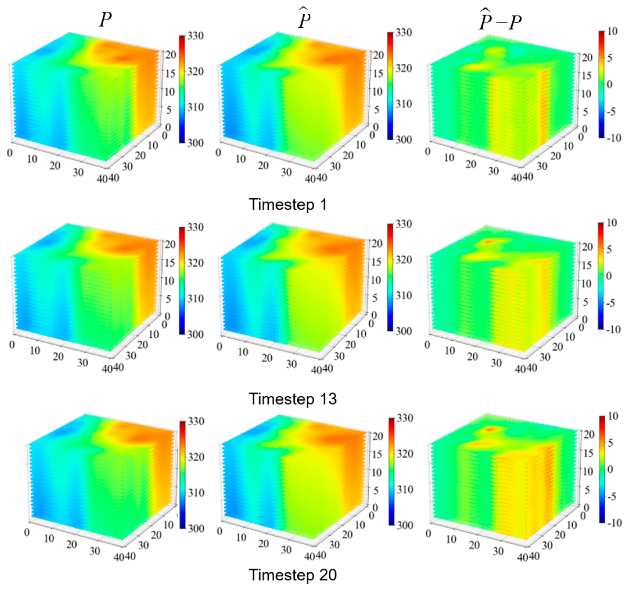
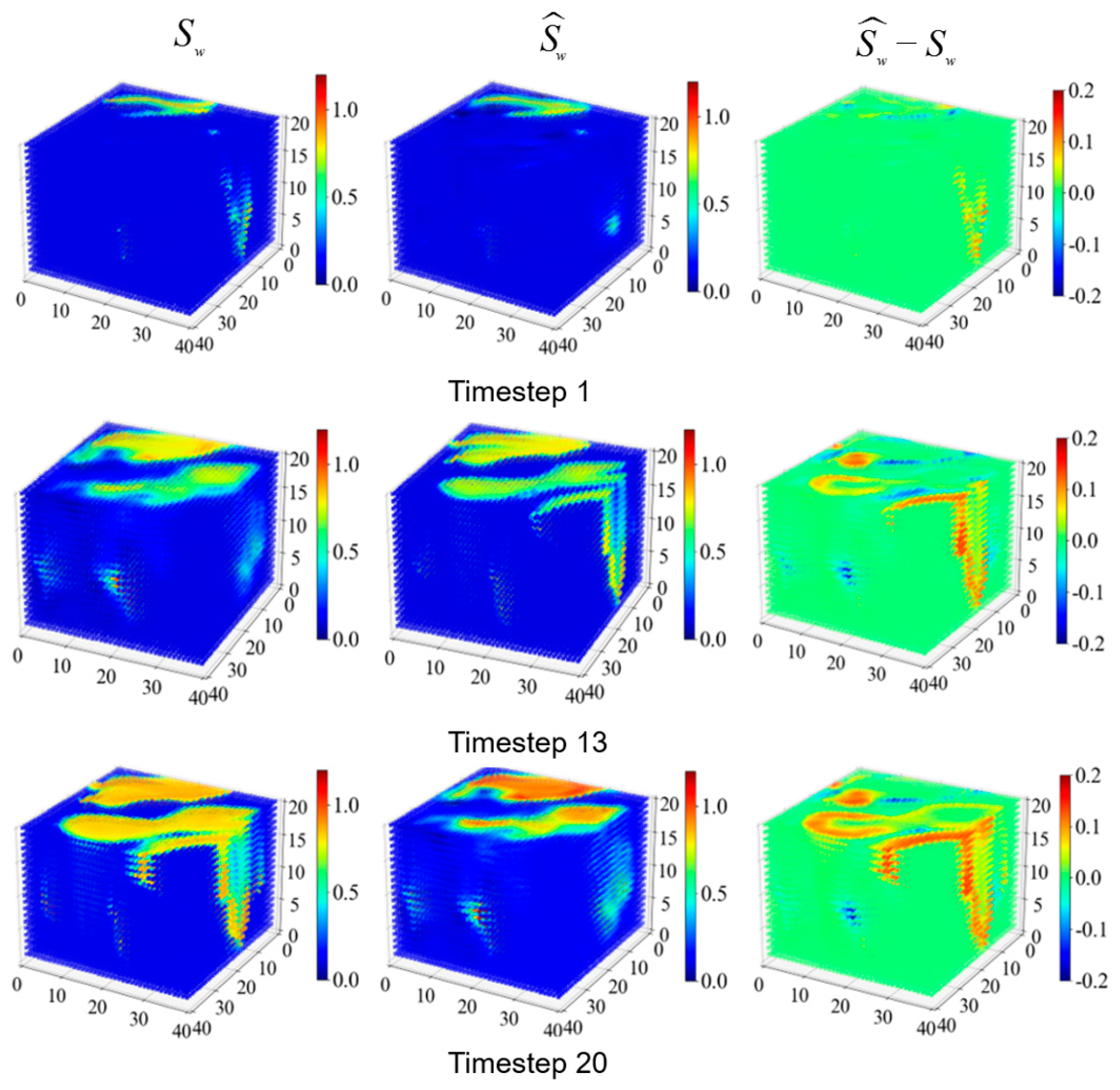
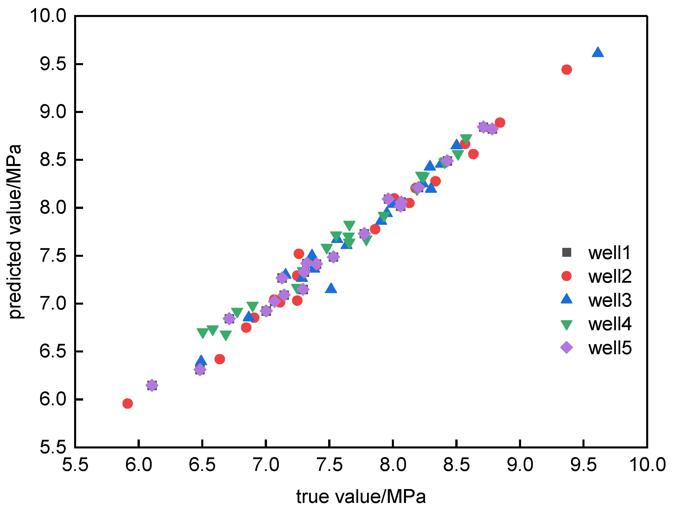
Figure 6 and Figure 7 are the surrogate model prediction results corresponding to the permeability in Figure 4. In Figure 6, it can be seen intuitively that the pressure distribution in steps 1, 13, and 20 (corresponding to 60, 780, and 1200 days) predicted by the surrogate model is in good agreement with the actual pressure distribution as a whole, especially the longitudinal pressure distribution. This shows that our CL-FNO has good performance for the long-term prediction of the 3D flow field. However, there is still a certain degree of error between the predicted and actual results of saturation in Figure 7, especially in the longitudinal direction, and this error tends to accumulate as prediction time increases. To further analyze the pressure prediction accuracy, Figure 8 shows the pressure fitting results of five observation points, where the x-axis is the actual value and the y-axis is the predicted value. It can be seen that the observation points are at or close to the line y = x, which indicates that the predicted value fits the actual value well. As can be seen in Table 2, the RMSE of the pressure and saturation are close for all samples, but the relative error of pressure field prediction is significantly lower than the saturation field error. In this regard, we make the following analysis: CL-FNO can predict the 3D saturation and pressure field, especially the long-term prediction of pressure, and still maintain good accuracy, which is the effect caused by the addition of physical constraints and cyclic gating functions at the same time. However, the larger relative error of saturation prediction may be due to the different “emphasis of error” of pressure and saturation, as the RMSEs of both reached a similar level, but there is still a gap between the field map and the MRE accuracy of the two. Therefore, saturation and pressure learning may not be suitable for backpropagation of the same set of loss functions, and they should probably be learned separately or coupled in a better way in a set of NN architectures.

3.2. Actual Reservoir Case

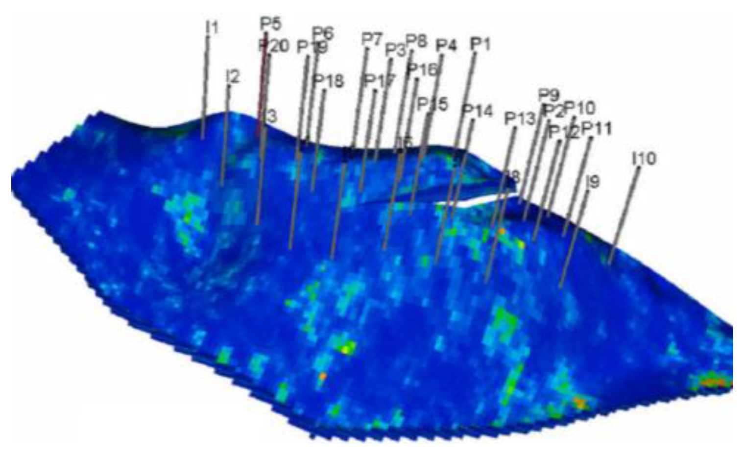
To validate the usability of the model in the actual oil field, the 3D CL-FNO model is applied to a real reservoir block case. The reservoir model is designed based on an actual water-flooding oil field, and the reservoir model has 60,048 (138 × 49 × 9) grid blocks with 44,550 active units. Figure 9 shows the actual logging permeability and well network. The northern edge of the reservoir has a large boundary fault and an internal fault with an angle of approximately 20° to the fault. The field has 20 producing wells and 10 injection wells, each with three injection sections. The reference permeability distribution and injection and production well locations are shown in Figure 9. The production well was controlled by the bottom hole pressure and injection wells were controlled by flow rate. The wells were shut down when the water cut exceeded 90%.
It is worth noting that the actual oil field was developed over a long period, and there is a large amount of historical data, including historical simulation data, which can be used in the training. This provides valuable direction for the reutilization of historical oil field data. Finally, we supplement part of the data with numerical simulation, which is used for training our model. The training flow of the actual case is the same as that of the synthetic case. In particular, the resolution of the input data is adaptively adjusted. The detailed neural network architecture used for the real case is shown in Table 3.
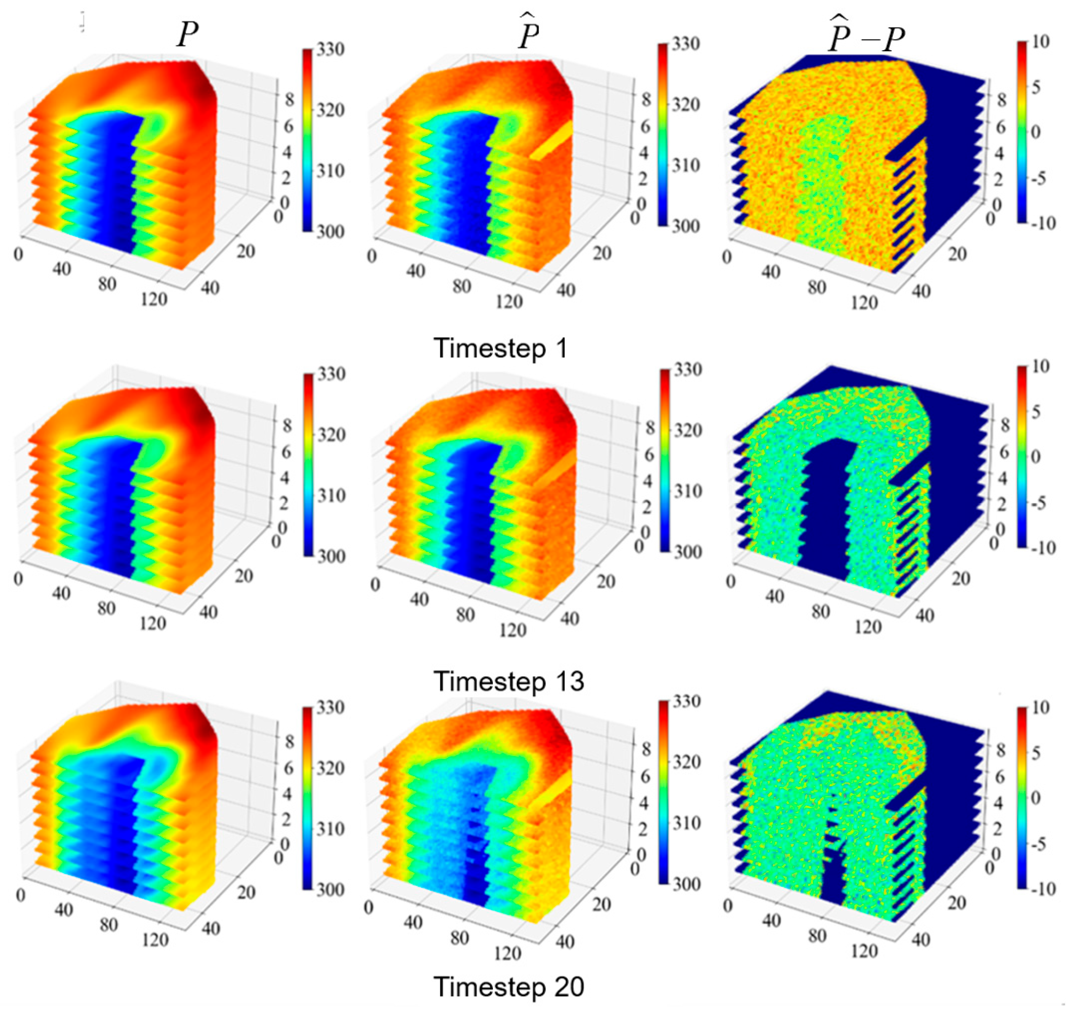
The pressure and saturation field distributions corresponding to the permeability field in Figure 9 are shown in Figure 10 and Figure 11. In Figure 10, the pressure prediction still intuitively agrees with the true value at time step 13; however, there is an observable error between them at time step 20. The pressure field can be accurately predicted over long time steps; however, after a longer time, there is a degree of divergence in the error. In Figure 11, the change in saturation is not very obvious; however, it can be observed that from the 13th time step, the prediction error begins to appear as a more obvious diffusion. Using 20% of the 800 training samples, we obtain the overall prediction error in Table 4; the RMSE and δ of saturation are larger, and its learning difficulty is greater than that of the pressure field. In particular, the δ of the pressure is also larger than that in the artificial model, indicating that the learning difficulty of the actual model is greater. In general, our improved 3D-FNO effectively realizes the pressure prediction of the actual complex 3D heterogeneous two-phase flow model. The overall error is controlled to within 10%, and the prediction error of the pressure field is controlled to within 5%, maintaining good accuracy during long-term prediction. The physically constrained machine learning model has great potential to assist with faster and more efficient reservoir dynamic prediction.

4. Conclusions

The fast and accurate prediction of oil–water two-phase flow in subsurface reservoirs is a crucial tool for enhancing the efficiency of engineering development. In this paper, a convolutional long short-term memory-Fourier neural operator (CL-FNO) model is proposed for 3D predictive model building, and the architecture is established by coupling the physical constraint with the spatio-temporal forecast. The performance of the model is validated using a synthetic model and an actual reservoir model:
  • A novel CL-FNO is designed based on the U-shaped architecture, combining the physical constraints Fourier neural operator, the temporal processing convolutional long short-term memory, and the spatial 3D convolution block.
  • A surrogate model is trained based on a synthetic numerical model and the CL-FNO is validated, exhibiting satisfactory long-term forecasting performance.
  • Based on an actual reservoir, a practical surrogate model is trained and the CL-FNO is demonstrated to possess the potential for addressing practical engineering requirements.
The CL-FNO realizes the prediction of the flow fields dynamic of the 3D oil–water two-phase flow in the heterogeneous reservoir, although there is still a problem in error divergence during longer-term prediction. In the future, we will conduct research on more advanced machine learning methods to further improve the accuracy and generalization ability.

Author Contributions

Conceptualization, K.Z.; Formal analysis, G.F.; Funding acquisition, K.Z.; Investigation, G.F.; Methodology, G.F.; Project administration, H.W., W.Y., Y.Z., J.L., P.L., L.Z., Y.Y., J.Y., A.L. and C.L.; Resources, K.Z.; Supervision, K.Z., H.W., W.Y., Y.Z., J.L., P.L., L.Z., Y.Y., J.Y., A.L. and C.L.; Validation, G.F.; Visualization, G.F.; Writing—original draft, G.F.; Writing—review and editing, G.F. and K.Z. All authors have read and agreed to the published version of the manuscript.

Funding

This work is supported by the National Natural Science Foundation of China under Grant 52325402, 52274057, 52074340, and 52374036; the National Key R&D Program of China under Grant 2023YFB4104200; the Major Scientific and Technological Projects of CNOOC under Grant CCL2022RCPS0397RSN; and the 111 Project under Grant B08028. The authors have no competing interests to declare that are relevant to the contents of this article. The datasets generated during the current study are available from the corresponding author upon reasonable request.

Data Availability Statement

The data presented in this study are available on request from the corresponding author.

Conflicts of Interest

Author Gaocheng Feng, Huan Wan, Weiying Yao and Ang Li was employed by the company CNOOC EnerTech-Drilling & Production Co.; Author Chen Liu was employed by the company CNOOC Research Institute Ltd. The remaining authors declare that the research was conducted in the absence of any commercial or financial relationships that could be construed as a potential conflict of interest. The remaining authors declare that the research was conducted in the absence of any commercial or financial relationships that could be construed as a potential conflict of interest.

References

  1. Krizhevsky, A.; Sutskever, I.; Hinton, G.E. ImageNet Classification with Deep Convolutional Neural Networks. Adv. Neural Inf. Process. Syst. 2012, 25. [Google Scholar] [CrossRef]
  2. LeCun, Y.; Bengio, Y.; Hinton, G. Deep learning. Nature 2015, 521, 436–444. [Google Scholar] [CrossRef] [PubMed]
  3. Wang, H.; Lin, X.; Jiang, L.; Liu, Z. An oilfield production prediction method based on clustering and long short-term memory neural network. Pet. Sci. Bull. 2023, 2023, 62–72. [Google Scholar]
  4. Tompson, J.; Schlachter, K.; Sprechmann, P.; Perlin, K. Accelerating eulerian fluid simulation with convolutional networks. In Proceedings of the 5th International Conference on Learning Representations, ICLR 2017, Toulon, France, 24–26 April 2017. [Google Scholar]
  5. Zha, W.; Li, D.; Shen, L.; Zhang, W.; Liu, X. Review of neural network-based methods for solving partial differential equations. Chin. J. Theor. Appl. Mech. 2022, 54, 543–556. [Google Scholar]
  6. Zhu, Y.; Zabaras, N. Bayesian deep convolutional encoder–decoder networks for surrogate modeling and uncertainty quantification. J. Comput. Phys. 2018, 366, 415–447. [Google Scholar] [CrossRef]
  7. Ma, T.; Xiang, G.; Shi, Y.; Gui, J.; Zhang, D. Horizontal in-situ stress prediction method based on the bidirectional long short-term memory neural network. Pet. Sci. Bull. 2022, 2022, 487–504. [Google Scholar]
  8. Tang, M.; Liu, Y.; Durlofsky, L.J. A deep-learning-based surrogate model for data assimilation in dynamic subsurface flow problems. J. Comput. Phys. 2020, 413, 109456. [Google Scholar] [CrossRef]
  9. Tang, M.; Liu, Y.; Durlofsky, L.J. Deep-learning-based surrogate flow modeling and geological parameterization for data assimilation in 3D subsurface flow. Comput. Methods Appl. Mech. Eng. 2021, 376, 113636. [Google Scholar] [CrossRef]
  10. Raissi, M.; Perdikaris, P.; Karniadakis, G.E. Physics-informed neural networks: A deep learning framework for solving forward and inverse problems involving nonlinear partial differential equations. J. Comput. Phys. 2019, 378, 686–707. [Google Scholar] [CrossRef]
  11. Li, Z.; Kovachki, N.; Azizzadenesheli, K.; Liu, B.; Bhattacharya, K.; Stuart, A.; Anandkumar, A. Fourier Neural Operator for Parametric Partial Differential Equations. In Proceedings of the International Conference on Learning Representations, Vienna, Austria, 4 May 2021. [Google Scholar]
  12. Wang, N.; Zhang, D.; Chang, H.; Li, H. Deep learning of subsurface flow via theory-guided neural network. J. Hydrol. 2020, 584, 124700. [Google Scholar] [CrossRef]
  13. Zhang, K.; Wang, Y.; Li, G.; Ma, X.; Cui, S.; Luo, Q.; Wang, J.; Yang, Y.; Yao, J. Prediction of Field Saturations Using a Fully Convolutional Network Surrogate. SPE J. 2021, 26, 1824–1836. [Google Scholar] [CrossRef]
  14. Zhang, K.; Zuo, Y.; Zhao, H.; Ma, X.; Gu, J.; Wang, J.; Yang, Y.; Yao, C.; Yao, J. Fourier Neural Operator for Solving Subsurface Oil/Water Two-Phase Flow Partial Differential Equation. SPE J. 2022, 27, 1815–1830. [Google Scholar] [CrossRef]
  15. Zhong, Z.; Sun, A.Y.; Yang, Q.; Ouyang, Q. A Deep Learning Approach to Anomaly Detection in Geological Carbon Sequestration Sites Using Pressure Measurements. J. Hydrol. 2019, 573, 885–894. [Google Scholar] [CrossRef]
  16. Huang, G.; Liu, Z.; Van Der Maaten, L.; Weinberger, K.Q. Densely Connected Convolutional Networks. In Proceedings of the IEEE Conference on Computer Vision and Pattern Recognition, Honolulu, HI, USA, 21–26 July 2017. [Google Scholar]
  17. Hochreiter, S.; Schmidhuber, J. Long Short-Term Memory. Neural Comput. 1997, 9, 1735–1780. [Google Scholar] [CrossRef] [PubMed]
  18. Gers, F.A.; Schmidhuber, J.; Cummins, F. Learning to Forget: Continual Prediction with LSTM. Neural Comput. 2000, 12, 2451–2471. [Google Scholar] [CrossRef] [PubMed]
  19. Lin, J.; Zhang, K.; Zhang, L.; Liu, P.; Peng, W.; Zhang, H.; Yan, X.; Liu, C.; Yang, Y.; Sun, H.; et al. Towards efficient and accurate CO2 sequestration optimization: Integrating hierarchical spatiotemporal information into deep-learning-based surrogate models. Fuel 2024, 356, 129343. [Google Scholar] [CrossRef]
  20. Guo, Y.; Cao, X.; Liu, B.; Gao, M. Solving Partial Differential Equations Using Deep Learning and Physical Constraints. Appl. Sci. 2020, 10, 5917. [Google Scholar] [CrossRef]
  21. Karumuri, S.; Tripathy, R.; Bilionis, I.; Panchal, J. Simulator-free solution of high-dimensional stochastic elliptic partial differential equations using deep neural networks. J. Comput. Phys. 2019, 404, 109120. [Google Scholar] [CrossRef]
  22. Zhu, Y.; Zabaras, N.; Koutsourelakis, P.-S.; Perdikaris, P. Physics-constrained deep learning for high-dimensional surrogate modeling and uncertainty quantification without labeled data. J. Comput. Phys. 2019, 394, 56–81. [Google Scholar] [CrossRef]
  23. Shi, X.; Chen, Z.; Wang, H.; Yeung, D.; Wong, W.; Woo, W. Convolutional LSTM network: A machine learning approach for precipitation nowcasting. Adv. Neural Inf. Process. Syst. 2015, 28. [Google Scholar] [CrossRef]
  24. Bianchi, M.; Zheng, C. SGeMS: A Free and Versatile Tool for Three-Dimensional Geostatistical Applications. Groundwater 2009, 47, 8–12. [Google Scholar] [CrossRef]
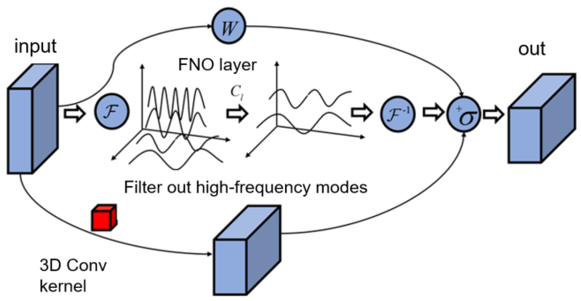
Figure 1. The block detail of the encoding process in CL-FNO.
Water 16 01411 g001
Figure 2. The block detail (a) and decoding sequence (b) of ConvLSTM in CL-FNO.
Water 16 01411 g002
Figure 3. Muti-layer structure of the CL-FNO architecture.
Water 16 01411 g003
Figure 4. Permeability field example and the well location in the synthetic model.
Water 16 01411 g004
Figure 5. The comparison of train and test loss between CL-FNO and ConvLSTM.
Water 16 01411 g005
Figure 6. 3D pressure field distribution of the synthetic model.
Water 16 01411 g006
Figure 7. 3D saturation field distribution of the synthetic model.
Water 16 01411 g007
Figure 8. Pressure fitting results at well grids.
Water 16 01411 g008
Figure 9. Permeability field distribution of the actual reservoir model.
Water 16 01411 g009
Figure 10. 3D pressure field distribution of the actual reservoir model.
Water 16 01411 g010
Figure 11. 3D saturation field distribution of the actual reservoir model.
Water 16 01411 g011
Table 1. Parameter settings for CL-FNO for synthetic case.
PortionDetailsData Size
Input data-40 × 40 × 20 × n
Encoding layer 13D Conv and 3D Fourier/Sum/ReLU40 × 40 × 20 × 16
Encoding layer 23D Conv and 3D Fourier/Sum/ReLU20 × 20 × 10 × 32
Encoding layer 33D Conv and 3D Fourier/Sum/ReLU10 × 10 × 5 × 32
Encoding layer 43D Conv and 3D Fourier/Sum/ReLU10 × 10 × 5 × 64
Intermediate layer 13D Fourier × 410 × 10 × 5 × 64
Intermediate layer 2ConvLSTM layer 10 × 10 × 5 × 64 × 20
Decoding layer 4Upsampling/Deconvolution/ReLU10 × 10 × 5 × 64 × 20
Decoding layer 3Upsampling/Deconvolution/ReLU10 × 10 × 5 × 32 × 20
Decoding layer 2Upsampling/Deconvolution/ReLU20 × 20 × 10 × 32 × 20
Decoding layer 1Upsampling/Deconvolution/ReLU40 × 40 × 20 × 32 × 20
Output data-40 × 40 × 20 × 1 × 20
Table 2. Reservoir saturation and pressure prediction errors.
ParameterRMSE δ /%
P0.06420.95
Sw0.06515.21
Table 3. Parameter settings for CL-FNO for actual reservoir case.
PortionDetailsData Size
Input data-138 × 49 ×9 × n
Encoding layer 13D Conv and 3D Fourier/Sum/ReLU138 × 49 ×9× 16
Encoding layer 23D Conv and 3D Fourier/Sum/ReLU69 × 25 × 5 × 32
Encoding layer 33D Conv and 3D Fourier/Sum/ReLU40 × 13 × 3 × 32
Encoding layer 43D Conv and 3D Fourier/Sum/ReLU40 × 13 × 3 × 64
Intermediate layer 13D Fourier × 440 × 13 × 3 × 64
Intermediate layer 2ConvLSTM layer 40 × 13 × 3 × 64 × 20
Decoding layer 4Upsampling/Deconvolution/ReLU40 × 13 × 3 × 64 × 20
Decoding layer 3Upsampling/Deconvolution/ReLU40 × 13 × 3 × 32 × 20
Decoding layer 2Upsampling/Deconvolution/ReLU69 × 25 × 5 × 32 × 20
Decoding layer 1Upsampling/Deconvolution/ReLU138 × 49 × 9 × 32 × 20
Output data-138 × 49 × 9 × 1 × 20
Table 4. 3D saturation field distribution of the actual reservoir model.
ParameterRMSE δ /%
P0.07472.46
Sw0.11517.23
Disclaimer/Publisher’s Note: The statements, opinions and data contained in all publications are solely those of the individual author(s) and contributor(s) and not of MDPI and/or the editor(s). MDPI and/or the editor(s) disclaim responsibility for any injury to people or property resulting from any ideas, methods, instructions or products referred to in the content.