Evaluation of High-Intensity Precipitation Prediction Using Convolutional Long Short-Term Memory with U-Net Structure Based on Clustering

Abstract

Recently, Asia has experienced significant damage from extreme precipitation events caused by climate change. Improving the accuracy of quantitative precipitation forecasts over wide regions is essential to mitigate the damage caused by precipitation-related natural disasters. This study compared the predictive performances of a global model trained on the entire dataset and a clustered model that clustered precipitation types. The precipitation prediction model was constructed by combining convolutional long short-term memory with a U-Net structure. Research data consisted of precipitation events recorded at 10 min intervals from 2017 to 2021, utilizing radar data covering the entire Korean Peninsula. The model was trained on radar precipitation data from 30 min before the current time (t − 30 min, t − 20 min, t − 10 min, and t − 0 min) to predict the precipitation after 10 min (t + 10 min). The prediction performance was assessed using the root mean squared error and mean absolute error for continuous precipitation data and precision, recall, F1 score, and accuracy for the presence or absence of precipitation. The research findings indicate that, with sufficient training data for each precipitation type, models trained on clustered precipitation types outperform those trained on the entire dataset, particularly for predicting high-intensity precipitation events.

1. Introduction

Recently, significant damage has occurred in Asia owing to extreme precipitation caused by climate change. On the Korean Peninsula, extreme precipitation manifests as localized heavy precipitation and flash floods, with high uncertainty in precipitation prediction. The increasing frequency of high-uncertainty precipitation events exacerbates challenges in water resource management and disaster prevention. To mitigate damage from precipitation-related natural disasters, such as flooding and dam overflow, there is a need to enhance the accuracy of quantitative precipitation forecasting (QPF) for extensive regions. In addition to surface precipitation observations, the use of precipitation radar data in QPF research has been increasing [1,2,3]. In addition, a high temporal resolution (short lead time) is essential for a rapid response to natural disasters. Short lead-time precipitation predictions are suitable as part of early warning systems. Recent estimations using machine learning have demonstrated superiority over traditional extrapolation methods in short lead times (1–10 min) [4,5]. Ayzel et al. predicted precipitation 5 min later using RainNet for nowcasting [2]. The machine learning approach of RainNet has outperformed Rainymotion (as a representative of standard tracking and extrapolation techniques based on optical flow).

Moreover, various studies have applied machine learning methods to enhance the accuracy of QPF models, proving excellent predictive performance in precipitation estimation [6,7,8,9,10,11]. Among the machine learning models, long short-term memory (LSTM) is widely used for predicting precipitation by capturing temporal patterns. Barrera-Animas et al. compared LSTM, XGBoost, and support vector regression for hourly precipitation prediction and found that LSTM exhibited the best performance [12]. Li et al. confirmed the excellent performance of precipitation runoff modeling using LSTM [13]. Poornima and Pushpalatha proposed a recurrent neural network (RNN)-based LSTM for precipitation prediction, demonstrating improved predictive performance compared to RNN and LSTM [14]. In addition, research is underway using a convolutional LSTM (ConvLSTM) to simulate spatial features within the LSTM. Yadav and Ganguly applied ConvLSTM to spatially distributed QPF (SD-QPF), which outperformed both the persistence and state-of-the-art methods using optical flow [15]. Shin et al. demonstrated the superior performance of machine learning in the QPF by applying radar data to convolutional long short-term memory with a U-Net structure (ConvLSTM2D U-Net) [16]. However, most precipitation prediction data pertain to low-intensity precipitation, leading to a slightly lower accuracy in predicting high-intensity precipitation. Given the importance of accurately predicting high-intensity precipitation in precipitation forecasting, it is necessary to classify precipitation to enhance predictive performance.

Precipitation occurs in various forms, each with distinct characteristics. Various clustering techniques have been employed to differentiate the precipitation patterns in radar data analyses [17,18,19,20]. Jo et al. applied self-organizing maps (SOMs) clustering as the first step to cluster the regional characteristics of precipitation, creating 100 SOMs clustered with a grid size of 10 × 10, followed by k-means clustering as the second step [21]. Owing to an excessive number of clusters generated by SOMs, we performed a secondary k-means clustering. In this study, we also conducted two rounds of clustering to ensure an adequate supply of training data. Zhang et al. divided precipitation into four types using k-means clustering and performed predictive modeling for eight major meteorological factors using LSTM [22]. The clustering of precipitation types and the construction of training models for each type are expected to improve the predictive performance. Predicting precipitation using training models tailored to specific precipitation types is anticipated to enhance overall accuracy.

In this study, we compared the predictive performance of a global model trained on an entire dataset with that of a clustered model that clustered precipitation types. Precipitation type clustering was conducted using two methods: first, by employing SOMs and k-means clustering to cluster precipitation into various types based on characteristics; second, by clustering precipitation into low- and high-intensity categories according to specific criteria. Furthermore, we compared the predictive performances based on data transformation. A precipitation prediction model was constructed by combining ConvLSTM2D U-Net. Research data consisted of precipitation events occurring at 10 min intervals from 2017 to 2021. Radar data covering the entire Korean Peninsula were used, and the model was trained on radar precipitation data from 30 min before the current time (t − 30 min, t − 20 min, t − 10 min, and t − 0 min) to predict the precipitation after 10 min (t + 10 min). The predictive performance was evaluated using the root mean squared error (RMSE) and mean absolute error (MAE) for continuous precipitation data and precision, recall, F1 score, and accuracy for classification of precipitation.

This paper is organized as follows. Section 2 describes the research methodology, including the clustering methods, convolutional neural network (CNN), ConvLSTM2D U-net, and evaluation metrics. Section 3 details the radar precipitation data used in this study. Chapter 4 shows the model learning process, and Chapter 5 compares the predictive performance of each comparative model. Chapter 6 discusses the limitations in the model learning process, and Chapter 7 summarizes the research findings and provides the conclusions.

2. Materials and Methods

2.1. Study Procedure

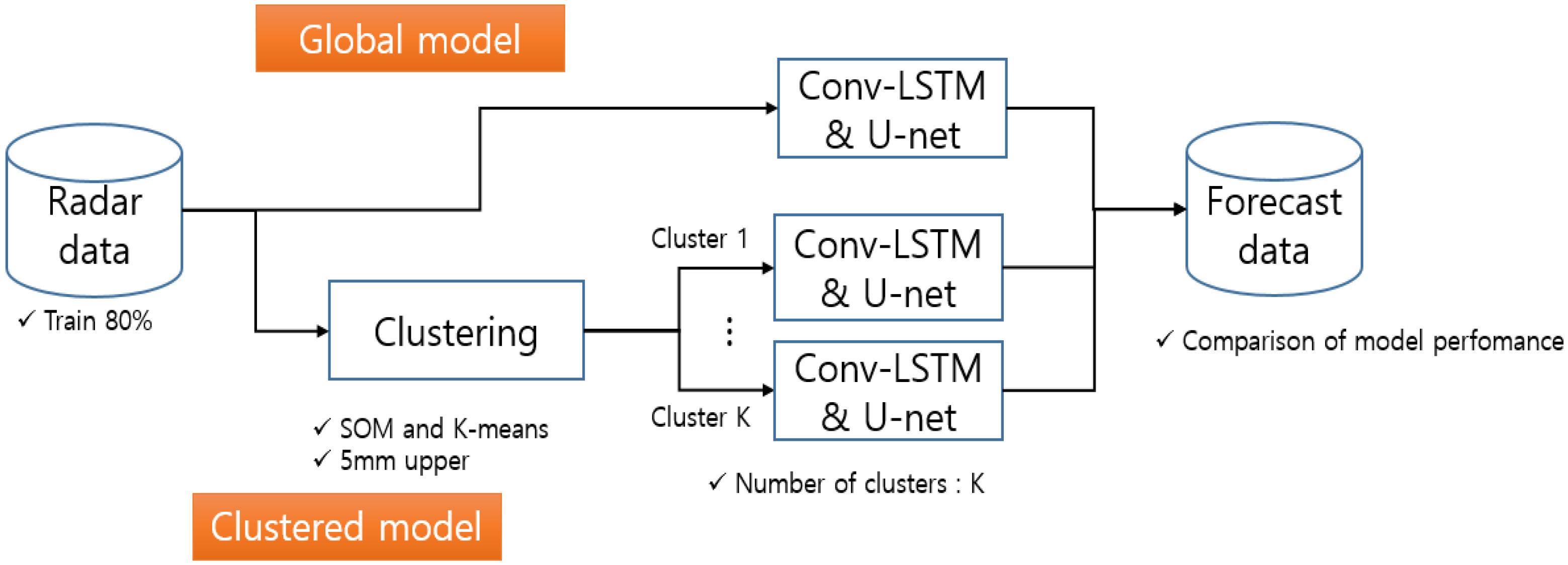
This study was conducted as shown in Figure 1. Data were divided into 80% for training and 20% for testing. The precipitation prediction model employs a ConvLSTM2D U-Net. Input data consisted of radar precipitation and cloud motion data from t − 30 min, t − 20 min, t − 10 min, and t − 0 min at 10 min intervals. These data were used to train the ConvLSTM2D U-net to predict the precipitation for the next 10 min (t + 10 min). Each model generated 10 outputs through 10-fold cross-validation and then ensembled the results to derive the precipitation prediction.

This study compared two approaches when training the ConvLSTM2D U-Net: a global model trained on all available training data and a clustered model trained on specific precipitation types clustered from training data. The precipitation type clustering was performed using two methods. First, SOM and k-means were employed to cluster precipitation types. SOM was applied as the first step for clustering training data, and clustering results were further subjected to second-step k-means clustering. Clustering results were also trained on a CNN to cluster precipitation types when new data were introduced. Second, precipitation was categorized as high or low intensity based on a threshold of 5 mm. The Korea Meteorological Administration issued heavy precipitation warnings if the accumulated precipitation exceeded 90 mm over 3 h. When converted into a 10 min interval, this threshold becomes 5 mm. Precipitation exceeding 5 mm was clustered as high intensity; otherwise, it was clustered as low intensity. The same 5 mm threshold was applied to cluster precipitation types for new data.

This study compared ten models by introducing changes in activation functions, data transformation, and clustering methods. The comparison models are presented in

Table 1. The study model.

Global Model	Design of ConvLSTM2D U-Net		Clustered Model	Clustering of Precipitation Pattern
	Precipitation Radar Data (10 min)	Activation Function		SOM	K-Means (Number of k)
G-M1	Raw data	ReLU	C-M1	10 × 10	3
			C-M2		4
G-M2	Normalization between 0 and 1 by min–max scaling		C-M3		3
G-M3	Log transformation of raw data	ELU	C-M4
G-M4		PreLU	C-M5
G-M1	Raw data	ReLU	C-M6	Whether high-intensity precipitation (5 mm and 10 min)

. G-M1 was trained using the ConvLSTM2D U-Net with rectified linear unit (ReLU) activation function, utilizing all raw data. C-M1 and C-M2 also use raw data but undergo clustering using SOM and k-means. In this case, C-M1 has 3 clusters, whereas C-M2 has 4 clusters. The activation function for both is ReLU. If min–max scaling is applied to all raw data in G-M1 for normalization, it becomes G-M2. C-M3 involves training the ConvLSTM2D U-Net on raw data clustered into three groups and normalized using min–max scaling. G-M3 and G-M4 involve log-transforming all raw data, and during training with ConvLSTM2D U-Net, they are divided based on the activation function, with G-M3 using exponential linear unit (ELU) and G-M4 using parametric ReLU (PReLU). Similarly, C-M4 and C-M5 cluster raw data into three groups and undergo log transformation, distinguishing between ELU and PreLU activation functions. C-M6 clusters data based on low- and high-intensity precipitation using the 5 mm and 10 min criteria.

2.2. Self-Organizing Map (SOM)

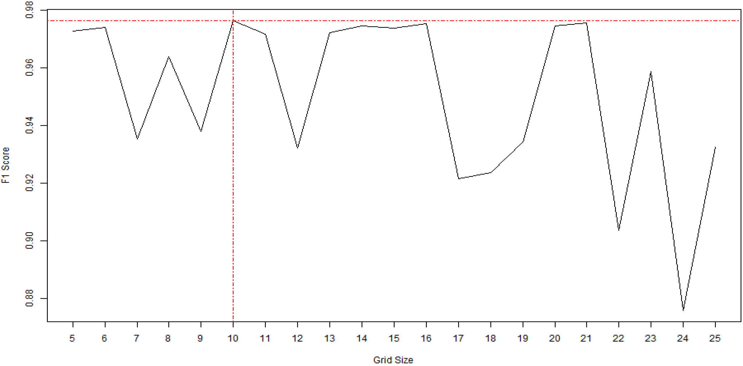
SOM, a type of artificial neural network, is a clustering technique that groups similar data with spatial characteristics, performing both dimensionality reduction and clustering. SOM is a neural network algorithm that can compress complex relationships between high-dimensional data into a two-dimensional array by comparing the Euclidean distances between input data [23,24]. To set the grid size, Tian et al. used $M\approx 5\sqrt{N}$ [25]. However, when there is a large amount of research data, setting too large of a grid size can lead to long computation times, which is a drawback. In this study, as it is important to have high clustering accuracy for prediction based on precipitation type, the grid size was selected using the representative F1 score metric (Figure 2). In this research, the grid size of SOM was set to 10 × 10 (Figure 3).

Radar imagery provides information on cloud movement, and simulating the formation and dissipation of precipitation is challenging. To address this, additional input data were generated to incorporate the occurrence of heavy precipitation and account for cloud formation and dissipation. Changes were calculated between the cumulative values at t − 30 min, t − 20 min, t − 10 min, and t − 0 min to capture the generation and dissipation of precipitation and its movement. Additionally, several non-zero grids were generated to assess the spatial extent of the precipitation. Furthermore, several grids with values exceeding 5 mm were generated to gauge precipitation intensity. This study employed the “kohonen”a package in R, and specifically the “supersom” function [26].

2.3. K-Means Clustering

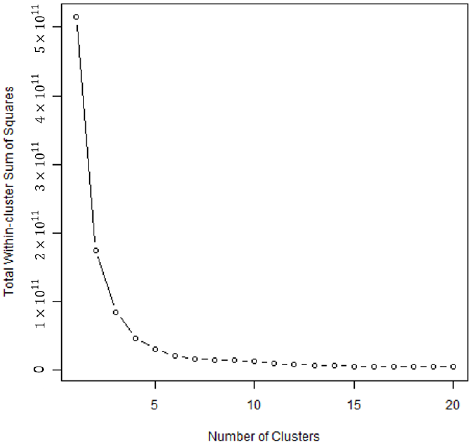
K-means clustering is the most commonly used method for clustering. It provides more accurate clustering results than SOMs [27]. Determining the number of clusters is essential for k-means clustering. The elbow method is one of the most prominent methods for determining the number of clusters. This method typically involves examining the within-cluster sum-of-squares (WSSs) based on the number of clusters to determine the appropriate number (Figure 4). In this study, the “kmeans” function in the “stats” package in R was utilized [27], and comparisons were made with three and four cluster numbers.

2.4. Convolutional Neural Network (CNN)

A CNN effectively recognizes features while preserving spatial information in images. It demonstrates a high performance in image clustering by extracting and clustering the features of an image [28]. The convolutional layer is the most crucial. The convolution in a two-dimensional plane of an image can be represented by the following equation:

$$\left(\mathit{f}\mathit{\ast }\mathit{g}\right)\left(\mathit{i},\mathit{j}\right)={\sum }_{\mathit{x}=\mathbf{0}}^{\mathit{h}-\mathbf{1}}{\sum }_{\mathit{y}=\mathbf{0}}^{\mathit{w}-\mathbf{1}}\mathit{f}\left(\mathit{x},\mathit{y}\right)\mathit{g}(\mathit{i}-\mathit{x},\mathit{j}-\mathit{y}),$$

where $h$ represents height, $w$ represents width, $f$ is the input, $\mathit{g}$ signifies the kernel, and $(f\ast g)$ results in the output.

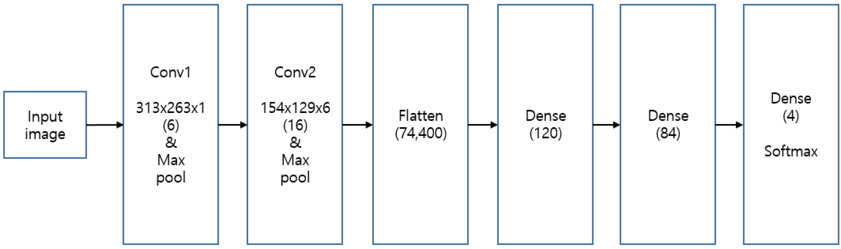
It is essential to first cluster the precipitation types to predict precipitation using a cluster model when new data are input. Therefore, the results of SOM and k-means clustering were trained on the CNN to appropriately cluster new radar images of precipitation. The CNN architecture consisted of two layers with (5, 5) kernels, followed by (2, 2) max pooling, and it utilized the Swish activation function. Finally, softmax activation is applied to the dense layer (Figure 5).

2.5. ConvLSTM2D U-Net

LSTM, an RNN, learns long-term dependencies by utilizing sequential information from the past. ConvLSTM, a model that applies CNN within LSTM, addresses the previous limitation of not being able to reflect spatial features effectively [29]. It simultaneously learns temporal and spatial characteristics through convolution operations instead of traditional matrix multiplications. The ConvLSTM designed by Shi et al. is defined as follows: it is designed with all the inputs $X_1, \cdots , X_t$, cell outputs $C_1, \cdots , C_t$, and hidden states $H_1, \cdots , H_t$ [29]. The gates $i_t$, $f_t$, $o_t$ are 3D tensors, where the last two dimensions are spatial.

$${\mathit{i}}_{\mathit{t}}=\mathit{\sigma }({\mathit{W}}_{\mathit{x}\mathit{i}}\mathit{\ast }{\mathit{X}}_{\mathit{t}}+{\mathit{W}}_{\mathit{h}\mathit{i}}\mathit{\ast }{\mathit{H}}_{\mathit{t}-\mathbf{1}}+{\mathit{W}}_{\mathit{c}\mathit{i}} ° {\mathit{C}}_{\mathit{t}-\mathbf{1}}+{\mathit{b}}_{\mathit{i}}),$$

$${\mathit{f}}_{\mathit{t}}=\mathit{\sigma }({\mathit{W}}_{\mathit{x}\mathit{f}}\mathit{\ast }{\mathit{X}}_{\mathit{t}}+{\mathit{W}}_{\mathit{h}\mathit{f}}\mathit{\ast }{\mathit{H}}_{\mathit{t}-\mathbf{1}}+{\mathit{W}}_{\mathit{c}\mathit{f}} ° {\mathit{C}}_{\mathit{t}-\mathbf{1}}+{\mathit{b}}_{\mathit{f}}),$$

$${\mathit{C}}_{\mathit{t}}={\mathit{F}}_{\mathit{t}} ° {\mathit{C}}_{\mathit{t}-\mathbf{1}}+{\mathit{i}}_{\mathit{t}} ° \mathbf{t}\mathbf{a}\mathbf{n}\mathbf{h}({\mathit{W}}_{\mathit{x}\mathit{c}}\mathit{\ast }{\mathit{X}}_{\mathit{t}}+{\mathit{W}}_{\mathit{h}\mathit{c}}\mathit{\ast }{\mathit{H}}_{\mathit{t}-\mathbf{1}}+{\mathit{b}}_{\mathit{c}}),$$

$${\mathit{o}}_{\mathit{t}}=\mathit{\sigma }({\mathit{W}}_{\mathit{x}\mathit{o}}\mathit{\ast }{\mathit{X}}_{\mathit{t}}+{\mathit{W}}_{\mathit{h}\mathit{o}}\mathit{\ast }{\mathit{H}}_{\mathit{t}-\mathbf{1}}+{\mathit{W}}_{\mathit{c}\mathit{o}} ° {\mathit{C}}_{\mathit{t}}+{\mathit{b}}_{\mathit{o}}),$$

$${\mathit{H}}_{\mathit{t}}={\mathit{o}}_{\mathit{t}} ° \mathbf{t}\mathbf{a}\mathbf{n}\mathbf{h}\left({\mathit{C}}_{\mathit{t}}\right),$$

where $\ast$ denotes the convolution operator and $°$ denotes the Hadamard product.

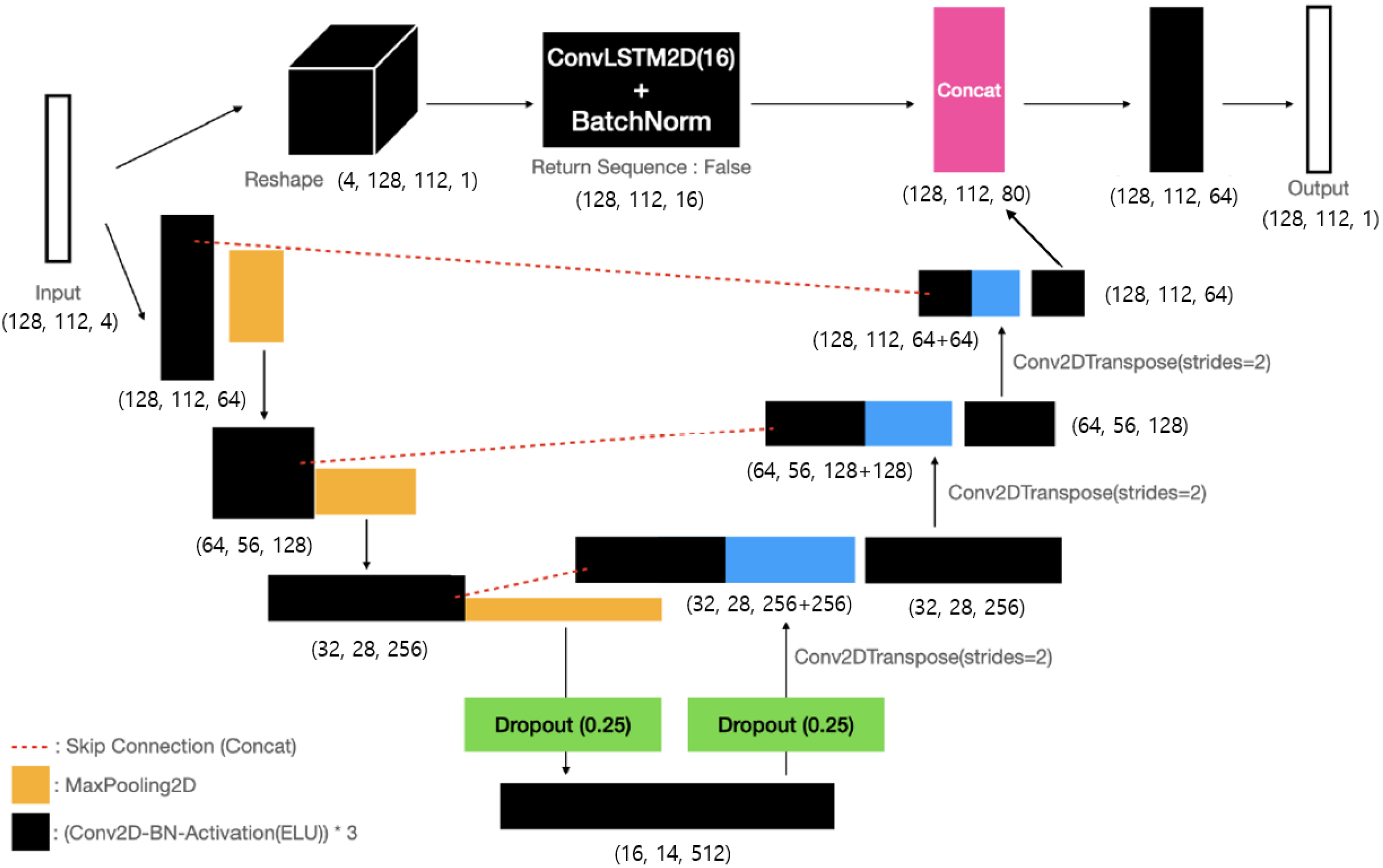
This study constructed a model to predict precipitation by incorporating a Conv-LSTM layer based on the U-Net architecture [16]. Here, the U-Net consists of a contracting path network to obtain the overall feature information of the image and an expanding path network for precise localization, forming a U-shaped symmetric structure. The Conv-LSTM model configuration includes using Conv2DTranspose layers with trained filters to increase the resolution through convolution operations. In addition, SpatialDropout2D was used to exclude all 2D feature maps. Specifically, a linear bottleneck structure is used to reduce the number of parameters. The bottleneck structure involves dimension reduction with a 1 × 1 convolution, followed by dimension expansion with a 3 × 3 convolution, and then using another 1 × 1 convolution to deepen the dimension, thereby effectively reducing the computational load. In this study, the input shape of the ConvLSTM2D U-Net models proposed by [16] was modified to (128, 112, 4) (Figure 6).

2.6. Performance Metrics

The radar precipitation data were continuous. RMSE and MAE were used to evaluate the predictive performance of continuous data. Here, $y_i$ represents the observed value and ${\widehat{y}}_i$ represents the predicted value. Additionally, to assess the presence or absence of precipitation, values below 0.01 were classified as “no precipitation,” and values equal to or above were classified as “precipitation”. In reality, “no precipitation” accounts for 11.3%, whereas precipitation accounts for 88.7%. The precision, recall, F1 score, and accuracy were used to evaluate the classification performance in the presence of precipitation.

$$\mathit{R}\mathit{M}\mathit{S}\mathit{E}=\sqrt{\frac{\mathbf{1}}{\mathit{n}}{\sum }_{\mathit{i}=\mathbf{1}}^{\mathit{n}}{\left({\mathit{y}}_{\mathit{i}}-{\widehat{\mathit{y}}}_{\mathit{i}}\right)}^{\mathbf{2}}}, \mathit{M}\mathit{A}\mathit{E}=\frac{\mathbf{1}}{\mathit{n}}{\sum }_{\mathit{i}=\mathbf{1}}^{\mathit{n}}|{\mathit{y}}_{\mathit{i}}-{\widehat{\mathit{y}}}_{\mathit{i}}|,$$

$$\mathit{P}\mathit{r}\mathit{e}\mathit{c}\mathit{i}\mathit{s}\mathit{i}\mathit{o}\mathit{n}=\frac{\mathit{T}\mathit{r}\mathit{u}\mathit{e}\mathit{P}\mathit{o}\mathit{s}\mathit{i}\mathit{t}\mathit{i}\mathit{v}\mathit{e}}{\mathit{T}\mathit{r}\mathit{u}\mathit{e}\mathit{P}\mathit{o}\mathit{s}\mathit{i}\mathit{t}\mathit{i}\mathit{v}\mathit{e}+\mathit{F}\mathit{a}\mathit{l}\mathit{s}\mathit{e}\mathit{P}\mathit{o}\mathit{s}\mathit{i}\mathit{t}\mathit{i}\mathit{v}\mathit{e}},$$

$$\mathit{R}\mathit{e}\mathit{c}\mathit{a}\mathit{l}\mathit{l}=\frac{\mathit{T}\mathit{r}\mathit{u}\mathit{e}\mathit{P}\mathit{o}\mathit{s}\mathit{i}\mathit{t}\mathit{i}\mathit{v}\mathit{e}}{\mathit{T}\mathit{r}\mathit{u}\mathit{e}\mathit{P}\mathit{o}\mathit{s}\mathit{i}\mathit{t}\mathit{i}\mathit{v}\mathit{e}+\mathit{F}\mathit{a}\mathit{l}\mathit{s}\mathit{e}\mathit{N}\mathit{e}\mathit{g}\mathit{a}\mathit{t}\mathit{i}\mathit{v}\mathit{e}},$$

$$\mathit{F}\mathbf{1}=\mathbf{2}\times \frac{\mathit{P}\mathit{r}\mathit{e}\mathit{c}\mathit{i}\mathit{s}\mathit{i}\mathit{o}\mathit{n}\times \mathit{R}\mathit{e}\mathit{c}\mathit{a}\mathit{l}\mathit{l}}{\mathit{P}\mathit{r}\mathit{e}\mathit{c}\mathit{i}\mathit{s}\mathit{i}\mathit{o}\mathit{n}+\mathit{R}\mathit{e}\mathit{c}\mathit{a}\mathit{l}\mathit{l}},$$

$$\mathit{A}\mathit{c}\mathit{c}\mathit{u}\mathit{r}\mathit{a}\mathit{c}\mathit{y}=\frac{\mathit{T}\mathit{r}\mathit{u}\mathit{e}\mathit{P}\mathit{o}\mathit{s}\mathit{i}\mathit{t}\mathit{i}\mathit{v}\mathit{e}+\mathit{T}\mathit{r}\mathit{u}\mathit{e}\mathit{N}\mathit{e}\mathit{g}\mathit{a}\mathit{t}\mathit{i}\mathit{v}\mathit{e}}{\mathit{A}\mathit{l}\mathit{l}}.$$

3. Data

In this study, radar precipitation data were utilized and synthesized from two-dimensional gridded precipitation data obtained from the S-band radar network operated by the Ministry of Environment. The Ministry of Environment oversees the operation of several radar installations, including Biseulsan mountain, Sobaeksan mountain, Mohusan mountain, Seodaesan mountain, Garisan mountain, Yebongsan mountain, and Gamaksan mountain (GAS) radars. These radars play a crucial role in monitoring precipitation within a 125 km observation radius. Nationally synthesized gridded radar precipitation data were utilized, combining data from six radars, excluding the GAS radar, which does not have the same operating period. The data period spanned from 2017 to 2021, focusing on events with recorded precipitation. To enhance the accuracy of precipitation predictions, a conditional merging technique that considers altitude effects was applied [30]. This process involved incorporating data from 604 ground rain-gauge stations. The complexity and volume of raw radar precipitation data were considered to facilitate the utilization of radar precipitation data in training; this was transformed into a multidimensional array data structure using the NumPy library. The temporal resolution of the data is 10 min intervals, and the spatial resolution was based on a 1 km grid, resulting in a 625 × 525 grid array. For analysis purposes, the spatial resolution of the data was further transformed into a 125 × 105 grid, summed at a 5 km grid interval. Research data comprised 22,161 samples, with 17,729 (80%) used as training data and 4432 (20%) as test data. Each NumPy array stored five radar precipitation data images for each training sample relative to the time points t − 30 min, t − 20 min, t − 10 min, t − 0 min, and t + 10 min (Figure 7).

4. Model Training

We achieved a global model by training ConvLSTM2D U-Net with all training data. Additionally, we categorized training data by precipitation type and trained the ConvLSTM2D U-Net to create clustered models. The MAE was used as the loss function during training, and the loss function was optimized for each model. Consequently, it was observed that G-M3 and C-M4 had a large MAE value, and the loss function did not converge. G-M2, G-M4, C-M3, and C-M5 showed rapid convergence but high MAE values. G-M1, C-M1, C-M2, and C-M6 demonstrated well-optimized loss functions.

The clustered models consisted of prediction models trained using ConvLSTM2D U-Net for each precipitation type. Therefore, it is necessary to first cluster the precipitation type to predict precipitation when new data are input. To cluster new data, we utilized the clustering results of the training data to train the CNN. Categorical cross-entropy was employed as the loss function for the CNN, and accuracy was used as a metric. Optimization of the loss function for CNN training was successful for all models.

C-M1, C-M2, C-M3, C-M4, and C-M5 predicted the precipitation types of test data using a CNN, whereas C-M6 clustered them based on the 5 mm criterion. The clustering results for training and test data are listed in

Table 2. The number of data by precipitation type.

Using SOM and k-Means Cluster
		Cluster 1	Cluster 2	Cluster 3
C-M1, C-M3, C-M4, C-M5	Train	1747 (9.9%)	4708 (26.6%)	11,274 (63.6%)
	Test	458 (10.3%)	1176 (26.5%)	2798 (63.1%)
	Precision: 0.986; Recall: 0.986; F1: 0.986; Accuracy: 0.986
		Cluster 1	Cluster 2	Cluster 3	Cluster 4
C-M2	Train	2688 (15.2%)	4465 (25.2%)	9729 (54.9%)	847 (4.8%)
	Test	674 (15.2%)	1123 (25.3%)	2409 (54.4%)	226 (5.1%)
	Precision: 0.983; Recall: 0.983; F1: 0.983; Accuracy: 0.983
Using 5 mm criteria
		Cluster 1		Cluster 2
C-M6	Train	10,576 (59.7%)		7153 (40.3%)
	Test	2677 (60.4%)		1755 (39.6%)

. When examining the cluster characteristics of C-M1, C-M3, C-M4, and C-M5, clusters 1, 2, and 3 were characterized by high-, moderate-, and by low-intensity precipitation, respectively. In C-M2, clusters 4, 1, and 3 were associated with high-, moderate-, and low-intensity precipitation, respectively. Cluster 3 in C-M2 also comprised low-intensity precipitation events, with precipitation amounts of <0.1 mm. In C-M6, cluster 1 represents low-intensity precipitation of <5 mm, whereas cluster 2 represents high-intensity precipitation of 5 mm or more.

For C-M1, C-M2, C-M3, C-M4, and C-M5, the clustering of precipitation types using SOM and k-means clustering resulted in clusters with too few data points. These clusters were presumed to have a limited impact on the training due to their small sizes. The high clustering accuracy observed in the CNN cluster prediction for the test data indicates that the precipitation types were well clustered.

G-M2 and C-M3 were trained with data that underwent min–max scaling using ConvLSTM2D U-Net; this led to a significant issue, in which the model tended to predict most data as 0. The actual values at t + 10 min indicate that non-zero grids account for 48.37% of the entire dataset. In contrast, the prediction results of G-M2 and C-M3 showed only 0.02% non-zero grids. Therefore, G-M2 and C-M3 were excluded from the comparison.

In machine learning, data normalization is performed to improve the learning performance. However, in G-M2 and C-M3, an issue arose wherein most of the data were predicted to be 0. In G-M3 and C-M4, data were transformed by performing a log transformation to achieve a distribution similar to the normal distribution for training. Due to the fact that a log transformation of zero resulted $-\infty$, it was replaced with a small value of $1\times {10}^{-10}$ for training purposes. Additionally, the ELU was used as the activation function due to negative values after log transformation. However, an issue emerged in G-M3 and C-M4, where the minimum value was 0.368, indicating a non-zero minimum. The range of ELU was $(-\alpha , \infty )$, and when $\alpha$ was estimated to be 1, it resulted in high values. To address this issue in G-M3 and C-M4, the PReLU was used as the activation function in G-M4 and C-M5. The PReLU range was $(-\infty , \infty )$, which allowed for sufficiently small predictions, resulting in a minimum value of 0. G-M3 and C-M4, having non-zero high values as their minimum, were excluded from the comparison.

$${\displaystyle ELU\left(x\right)=\left\{\begin{array}{cc}\hfill x, & x>0\hfill \\ \hfill \alpha (e^x-1), & x\le 0\hfill \end{array}\right., PReLU(x)=\left\{\begin{array}{cc}\hfill x, & x\ge 0\hfill \\ \hfill \alpha x, & x<0\hfill \end{array}\right..}$$

5. Results

The performance of each model in predicting precipitation levels is presented in

Table 3. Results of RMSE and MAE.

	All Precipitation Events		High-Intensity Precipitation Events
	RMSE	MAE	RMSE	MAE
G-M1	0.107	0.020	1.339	1.137
G-M4	0.136	0.024	1.798	1.527
C-M1	0.109	0.021	1.352	1.150
C-M2	0.111	0.021	1.384	1.182
C-M5	0.193	0.029	2.701	2.173
C-M6	0.108	0.020	1.336	1.133

. For all types of precipitation, G-M1 demonstrated the best performance, with an RMSE of 0.107 and an MAE of 0.020. C-M1 and C-M6 exhibited similar and commendable performances, with RMSE values of 0.109 and 0.108.

Socioeconomic damage resulting from precipitation occurs mainly in heavy rather than light precipitation cases. Therefore, predictive accuracy for heavy precipitation is crucial. The criterion for heavy precipitation alerts by the Korea Meteorological Administration is 3 h accumulated precipitation of 90 mm or more, equivalent to 5 mm at 10 min intervals. We assessed the predictive performance of the grid cells with actual values exceeding 5 mm for each test dataset. C-M6 demonstrated the best performance with an RMSE of 1.336 and an MAE of 1.133. G-M1, which exhibited the best predictive performance for the entire precipitation dataset, had an RMSE of 1.339 for high-intensity precipitation, which was similar to C-M6 but slightly inferior. In other words, C-M6, which clustered precipitation types, demonstrated the most superior predictive performance for high-intensity precipitation.

We examined the classification accuracy to determine the accuracy of predicting precipitation within grids and the presence or absence of precipitation for the precipitation prediction results of each model. Numerical values within grids < 0.01 were classified as “no precipitation,” whereas those ≥0.01 were classified as “precipitation”. The classification accuracy was assessed using precision, recall, F1-score, and accuracy. Results of classification accuracy for precipitation using the model are shown in

Table 4. Metrics of the presence/absence of precipitation of various models.

	Precision	Recall	F1	Accuracy
G-M1	0.907	0.872	0.888	0.983
G-M4	0.890	0.886	0.887	0.983
C-M1	0.910	0.862	0.884	0.982
C-M2	0.905	0.866	0.884	0.982
C-M5	0.865	0.897	0.880	0.981
C-M6	0.912	0.862	0.885	0.983

. Overall, a high classification accuracy was observed. G-M1 exhibited the highest classification accuracy in terms of F1 score and accuracy, whereas C-M6 exhibited the highest precision and accuracy. The model with the highest recall is C-M5. G-M1 and C-M6 have demonstrated excellent performance in classifying precipitation presence or absence.

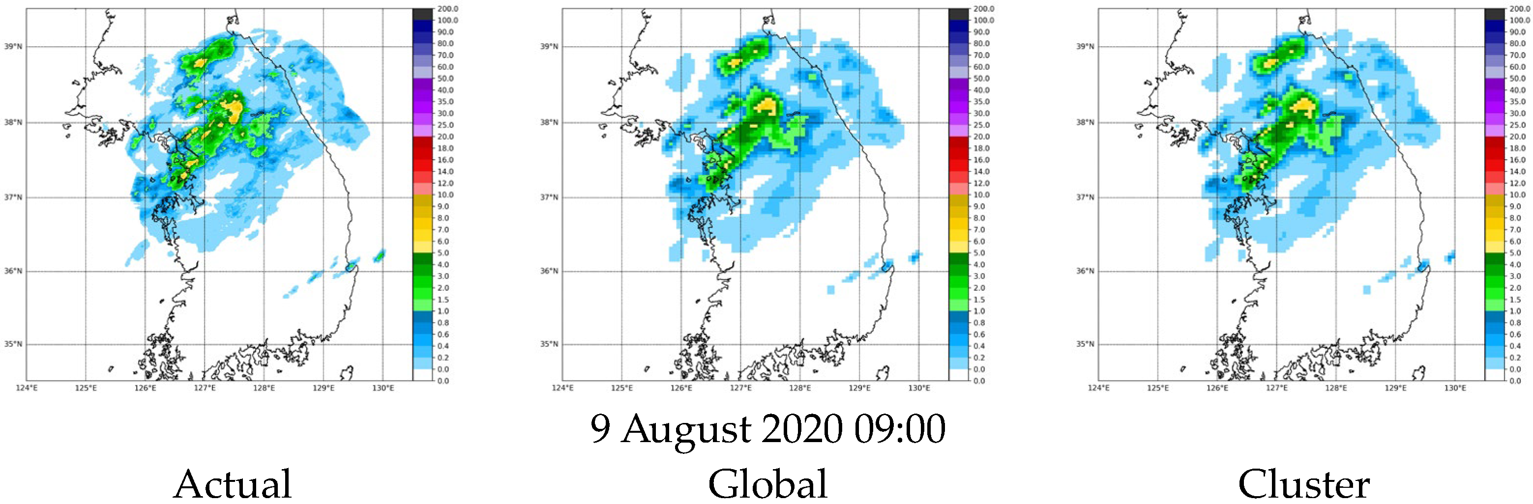
We examined the predictive performance of G-M1 and C-M6. We observed a linear relationship in the scatter plots against actual values (Figure 8). In addition, we observed a similar pattern in the predictions by visualizing the days with intense precipitation, as shown in Figure 9.

6. Discussion

If precipitation types are clustered and learned, it is possible to predict precipitation appropriate for that type. However, because certain types of events are small, the amount of training is reduced, and predictions are affected. The main focus should be on dangerous high-intensity precipitation. Therefore, it is necessary to collect and learn from a variety of high-intensity precipitation events. Additionally, in this study, min–max scaling and log transformation were performed to normalize data. However, prediction performance tended to decline. If data exhibit a zero-inflated distribution, normalization tends to reduce the difference with zero values, making zero more dominant. Consequently, this leads to the issue of predicting values close to zero. Further research on a learning method that can properly utilize the characteristics of precipitation data with many incidents of “no precipitation” is required.

7. Conclusions

It is essential to enhance the prediction accuracy of high-intensity precipitation events to prevent damage from extreme precipitation events. This study simulated the process of improving predictive performance for high-intensity precipitation by clustering precipitation types. ConvLSTM2D U-Net models were trained based on the clustered precipitation types and compared with a global model that did not cluster precipitation types.

The global model (G-M1), trained on the entire precipitation dataset using ConvLSTM2D U-Net with ReLU activation function, exhibited excellent predictive performance. However, models that clustered precipitation types using SOM and k-means clustering showed inferior performance. When performing clustering of precipitation types using SOM and k-means clustering, each cluster contains a very small amount of data; this leads to a reduced number of training samples, impacting the training of ConvLSTM2D U-Net, resulting in a lower predictive performance. The C-M6 model, which clustered precipitation types based on a criterion of 5 mm precipitation demonstrated excellent performance similar to the global model (G-M1). This is attributed to a sufficient number of training data for each cluster, in contrast to SOM and k-means clustering. Furthermore, it exhibited superior predictive performance for high-intensity precipitation compared to the global model (G-M1). Additionally, the classification accuracy for the presence or absence of precipitation also showed high accuracy.

In summary, the ConvLSTM2D U-Net model trained on the entire dataset performed well in predicting precipitation. However, its performance in predicting high-intensity precipitation was slightly lower. In contrast, models trained on the clustered precipitation types showed improved predictive performance for high-intensity precipitation. Therefore, there is a need to cluster precipitation types to enhance the performance of prediction of high-intensity precipitation. In the future, with the accumulation of more precipitation data, an increase in training data for each precipitation type is expected, leading to an even better predictive performance.

References

- Agrawal, S.; Barrington, L.; Bromberg, C.; Burge, J.; Gazen, C.; Hickey, J. Machine learning for precipitation nowcasting from radar images. arXiv 2019, arXiv:1912.12132. [Google Scholar] [CrossRef]
- Ayzel, G.; Scheffer, T.; Heistermann, M. RainNet v1. 0: A convolutional neural network for radar-based precipitation nowcasting. Geosci. Model Dev. 2020, 13, 2631–2644. [Google Scholar] [CrossRef]
- Peng, X.; Li, Q.; Jing, J. CNGAT: A Graph Neural Network Model for Radar Quantitative Precipitation Estimation. IEEE Trans. Geosci. Remote Sens. 2021, 60, 5106814. [Google Scholar] [CrossRef]
- Tran, Q.K.; Song, S.K. Computer vision in precipitation nowcasting: Applying image quality assessment metrics for training deep neural networks. Atmosphere 2019, 10, 244. [Google Scholar] [CrossRef]
- Yoon, S.; Park, H.; Shin, H. Very short-term rainfall prediction based on radar image learning using deep neural network. J. Korea Water Resour. Assoc. 2020, 53, 1159–1172. [Google Scholar] [CrossRef]
- Chen, M.; Li, Z.; Gao, S.; Xue, M.; Gourley, J.J.; Kolar, R.L.; Hong, Y. A flood predictability study for Hurricane Harvey with the CREST-iMAP model using high-resolution quantitative precipitation forecasts and U-Net deep learning precipitation nowcasts. J. Hydrol. 2022, 612, 128168. [Google Scholar] [CrossRef]
- Zhao, Q.; Liu, Y.; Yao, W.; Yao, Y. Hourly rainfall forecast model using supervised learning algorithm. IEEE Trans. Geosci. Remote Sens. 2021, 60, 4100509. [Google Scholar] [CrossRef]
- Grace, R.K.; Suganya, B. Machine learning based rainfall prediction. In Proceedings of the 2020 6th International Conference on Advanced Computing and Communication Systems, Chengdu, China, 11–14 December 2020; pp. 227–229. [Google Scholar] [CrossRef]
- Salehin, I.; Talha, I.M.; Hasan, M.M.; Dip, S.T.; Saifuzzaman, M.; Moon, N.N. An Artificial intelligence based rainfall prediction using LSTM and neural network. In Proceedings of the 2020 IEEE International Women in Engineering (WIE) Conference on Electrical and Computer Engineering, Bhubaneswar, India, 26–27 December 2020; pp. 5–8. [Google Scholar] [CrossRef]
- Basha, C.Z.; Bhavana, N.; Bhavya, P.; Sowmya, V. Rainfall prediction using machine learning & deep learning techniques. In Proceedings of the 2020 International Conference on Electronics and Sustainable Communication Systems, Coimbatore, India, 2–4 July 2020; pp. 92–97. [Google Scholar] [CrossRef]
- Yen, M.H.; Liu, D.W.; Hsin, Y.C.; Lin, C.E.; Chen, C.C. Application of the deep learning for the prediction of rainfall in Southern Taiwan. Sci. Rep. 2019, 9, 12774. [Google Scholar] [CrossRef]
- Barrera-Animas, A.Y.; Oyedele, L.O.; Bilal, M.; Akinosho, T.D.; Delgado, J.M.D.; Akanbi, L.A. Rainfall prediction: A comparative analysis of modern machine learning algorithms for time-series forecasting. Mach. Learn. Applic. 2022, 7, 100204. [Google Scholar] [CrossRef]
- Li, W.; Kiaghadi, A.; Dawson, C. High temporal resolution rainfall–runoff modeling using long-short-term-memory (LSTM) networks. Neur. Comput. Appl. 2021, 33, 1261–1278. [Google Scholar] [CrossRef]
- Poornima, S.; Pushpalatha, M. Prediction of rainfall using intensified LSTM based recurrent neural network with weighted linear units. Atmosphere 2019, 10, 668. [Google Scholar] [CrossRef]
- Yadav, N.; Ganguly, A.R. A deep learning approach to short-term quantitative precipitation forecasting. In Proceedings of the 10th International Conference on Climate Informatics, Virtually, 23–25 September 2020; pp. 8–14. [Google Scholar]
- Shin, H.; Yoon, S.; Choi, J. Radar rainfall prediction based on deep learning considering temporal consistency. J. Korea Water Resour. Assoc. 2021, 54, 301–309. [Google Scholar] [CrossRef]
- Kristollari, V.; Karathanassi, V. Fine-Tuning Self-Organizing Maps for Sentinel-2 Imagery: Separating Clouds from Bright Surfaces. Remote Sens. 2020, 12, 1923. [Google Scholar] [CrossRef]
- Harsono, T.; Basuki, A. Cloud satellite image segmentation using meng hee heng k-means and dbscan clustering. In Proceedings of the 2018 International Electronics Symposium on Knowledge Creation and Intelligent Computing, Surabaya, East Java, Indonesia, 29–30 October 2018; pp. 367–371. [Google Scholar] [CrossRef]
- Ferawati, K. Statistical Clustering of Heavy Precipitation Radar Images in Surabaya Using Gaussian Mixture Model. Ph.D. Thesis, Institut Teknologi Sepuluh Nopember, Surabaya, Indonesia, 2018. [Google Scholar]
- Huang, P.H.; Chou, W.C.; Lin, W.T. Using SOM and DBSCAN-based models for landslide hazard and spatial correlations analysis: A case study in central Taiwan. In Proceedings of the 2012 20th International Conference on Geoinformatics, Hong Kong, China, 15–17 June 2012; pp. 1–5. [Google Scholar] [CrossRef]
- Jo, E.; Park, C.; Son, S.W.; Roh, J.W.; Lee, G.W.; Lee, Y.H. Classification of localized heavy rainfall events in South Korea. Asia-Pac. J. Atmos. Sci. 2020, 56, 77–88. [Google Scholar] [CrossRef]
- Zhang, C.J.; Zeng, J.; Wang, H.Y.; Ma, L.M.; Chu, H. Correction model for rainfall forecasts using the LSTM with multiple meteorological factors. Meteorol. Appl. 2020, 27, e1852. [Google Scholar] [CrossRef]
- Kohonen, T. The self-organizing map. Proc. IEEE 1990, 78, 1464–1480. [Google Scholar] [CrossRef]
- Vesanto, J.; Alhoniemi, E. Clustering of the self-organizing map. IEEE Trans. Neur. Netw. 2000, 11, 586–600. [Google Scholar] [CrossRef]
- Tian, J.; Azarian, M.H.; Pecht, M. Anomaly detection using self-organizing maps-based k-nearest neighbor algorithm. PHM Soc. Eur. Conf. 2014, 2. [Google Scholar]
- Wehrens, R.; Kruisselbrink, J. Flexible self-organizing maps in kohonen 3.0. J. Stat. Softw. 2018, 87, 1–18. [Google Scholar] [CrossRef]
- Hartigan, J.A.; Wong, M.A. Algorithm AS 136: A k-means clustering algorithm. J. R. Stat. Soc. 1979, 28, 100–108. [Google Scholar] [CrossRef]
- Krizhevsky, A.; Sutskever, I.; Hinton, G.E. ImageNet classification with deep convolutional neural networks. Commun. ACM 2018, 60, 84–90. [Google Scholar] [CrossRef]
- Shi, X.; Chen, Z.; Wang, H.; Yeung, D.Y.; Wong, W.K.; Woo, W.C. Convolutional LSTM network: A machine learning approach for precipitation nowcasting. Adv. Neur. Inf. Process. Syst. 2015, 28. [Google Scholar]
- Yoon, S.S.; Bae, D.H. Optimal rainfall estimation by considering elevation in the Han River Basin, South Korea. J. Appl. Meteorol. Clim. 2013, 52, 802–818. [Google Scholar] [CrossRef]