Groundwater Responses of Foundation Subjected to Water Level Fluctuation of Reservoir Considering Variability of Layered Structure

Abstract

The effect of the variability in a layered structure, characterized by the spatial variability of the saturated hydraulic conductivity, on the distribution of a pressure head $p$ in a foundation subjected to water level fluctuation in a reservoir is investigated with the aid of the random field theory, Karhunen–Loève (K-L) expansion, first-order moment approach, and cross-correlation analysis. The results show that the variability in the foundation structure has significant impacts on the groundwater response to the reservoir’s water level fluctuations. Regions with relatively large uncertainties of the $p$ and ${\sigma }_p$ values in the foundation are those around the initial water level at the reservoir side, and those at the distal end away from the reservoir. In addition, there is a larger variance of $K_s$, denoted as ${\sigma }_{ln{K}_s}^2$, a larger correlation scale in the horizontal direction ${\lambda }_h$, a larger correlation scale in the vertical direction ${\lambda }_v$, and a larger one-way time consumption of fluctuations T to a larger uncertainty in $p$. Moreover, the four factors (${\sigma }_{ln{K}_s}^2$, ${\lambda }_h$, ${\lambda }_v$, and $T$) all have positive correlations with ${\sigma }_p$. ${\sigma }_{ln{K}_s}^2$ has the largest impact on ${\sigma }_p$ in the foundation, ${\lambda }_v$ has the second largest impact, and ${\lambda }_h$ has the smallest impact. A foundation with small $K_s$ values around the initial water level at the reservoir side and large $K_s$ values around the highest water level at the reservoir side may produce larger $p$ values in the foundation. These results yield useful insight into the effect of the variability in a layered structure on the distribution of the pressure head in a foundation subjected to water level fluctuation in a reservoir.

1. Introduction

Due to the water level scheduling of reservoirs, groundwater in foundations of buildings along the reservoir is inevitably impacted and changes accordingly. The water level fluctuations in a reservoir can cause changes in the hydraulic head, which is the pressure exerted by the groundwater. These changes in the hydraulic head can induce seepage flows through the soil and affect the stability and performance of foundations [1,2]. The magnitude and duration of the water level fluctuations, as well as the permeability characteristics of the soil, can influence the extent of these groundwater responses. For example, due to the rise and fall scheduling of the Three Gorges reservoir in China, the foundations of buildings along the reservoir remain under water level fluctuations for a long time. The impact of the fluctuating water level on the foundation is inevitable, which generally leads to the softening of the foundation and a decrease in the stability of the foundation [3]. Thus, it is of great significance to grasp the law of groundwater response in a foundation subjected to reservoir level fluctuations.

Currently, the engineering community commonly considers the “capillary rise height combined with the depth at which the foundation is buried” as the accepted criterion for determining the critical depth at which a building may be submerged without significant structural damage [4]. However, it is important to note that this criterion is just one aspect of assessing the critical depth of submergence for buildings and should be used in conjunction with other engineering considerations. Factors such as soil type, groundwater conditions, hydrostatic pressure, and the specific design and construction of the building can greatly influence its ability to withstand submergence. For foundations subjected to water level fluctuation in the reservoir, this criterion may not fully consider the rise and fall of the water table and its effect on groundwater distribution. For example, although both the capillary rise height and the footing burial depth have been considered when determining the critical depth in the footing design, the deformation of the foundation and impact on buildings still occurred along the reservoir even when the groundwater did not directly submerge the footing. Hence, further investigation into the groundwater responses in foundations subjected to reservoir water level fluctuations is necessary to ensure the safety and performance of structures in such environments.

The groundwater response to reservoir water level fluctuations highly depends on the foundation of the soil structures [5,6]. However, in many cases, the focus is often on the characteristics of water level fluctuations and the general properties of the foundation, and the specific soil structure is not considered. The soil structure plays a crucial role in determining the behavior of groundwater in foundations. Heterogeneous soil layers, variations in permeability, and the presence of geological features such as fractures or faults can significantly impact the groundwater flow and response to reservoir water level fluctuations. Neglecting these factors can lead to incomplete or inaccurate assessments of the groundwater behavior.

Layered soil foundations are commonly seen along reservoirs [7]. In natural layered soil foundations, the engineering properties of coarse-grained soils (such as gravel, pebble, gravelly soil, and medium-coarse sand) generally remain relatively unchanged in their natural or saturated states. However, these coarse-grained soils can act as preferential pathways for water ingress, surrounding the fine-grained soils (such as fine sand, silt, and clay) that experience significant reductions in their mechanical properties when saturated. In this case, how the groundwater changes with the water level variation in a reservoir remain unexplored, which is crucial for a foundation stability analysis. In addition, due to the heterogeneous nature of the geology [8,9,10], the soil layers may not be fully extended but vary in length and thickness; this makes the seepage and moisture distribution much more complex under the groundwater fluctuation scenario. This further leads to differential deformation (e.g., uneven subsidence) and poses a potential threat to the foundation’s stability. Therefore, it is necessary to conduct an in-depth study on the influence on the foundation’s groundwater distribution brought by the water level change while considering the variability of layered structures.

While many studies have focused on the bearing capacity issues of foundations subjected to water level changes [1,2,3,4] or the spatial variability of mechanical parameters [11,12,13,14,15], the groundwater responses, considering the spatial variability of hydraulic parameters, are more fundamental to these issues when the foundation is subjected to reservoir water level fluctuation and hence should be tackled first. To this aim, the objective of this study is to provide a better understanding of the groundwater responses of a foundation subjected to water level fluctuation in a reservoir while considering the variability of the layered structure. The variability of the layered structure of a foundation is characterized by the spatial variability of the saturated hydraulic conductivity $K_s$. To achieve this objective, we first illustrate the impacts of the foundation structures on the groundwater response subjected to the reservoir water level fluctuations by generating deterministic layered $K_s$ fields with different degrees of layering, and their transient seepages subjected to water level fluctuations are analyzed through the phreatic surface, pressure head, and streamlines to delineate the groundwater response law. Afterwards, to consider the variability of the layered structure, the probabilistic description of the layered structure is introduced based on the random field theory. With this probabilistic framework, the uncertainty in groundwater responses resulting from the variability in the layered structure of the foundation is evaluated using the first-order moment approach. Furthermore, to reveal the spatial relationship between the pressure head and the soil structures in the foundation, the cross-correlation between $p$ at any one observation point and $K_s$ values at every element in the foundations are derived through the cross-correlation analysis.

2. Methodology

2.1. Basic Equations

The groundwater responses in the layered foundation subjected to water level fluctuation in reservoir can be described by a two-dimensional governing flow equation:

$$\frac{\partial }{\partial x}\left(K\left(p\right)\frac{\partial p}{\partial x}\right)+\frac{\partial }{\partial z}\left(K\left(p\right)\left(\frac{\partial p}{\partial z}+1\right)\right)=\left[\eta S_s+C(p)\right]\frac{\partial p}{\partial t}$$

(1)

where x and z denote the coordinates along the horizontal x-axis and vertical z-axis, respectively; $p$ is the pressure head; $K\left(p\right)$ is the hydraulic conductivity; $S_s$ is the specific storage; $C\left(p\right)$ denotes the moisture capacity term; $t$ denotes time; and $\eta$ is the saturation index. $p$ is positive if the medium is fully saturated, and it is negative if the medium is unsaturated. $K\left(p\right)$ varies with pressure head $p$ under unsaturated conditions. $S_s$ represents the percentage of water released from a unit volume of fully saturated porous media under a unit decline in hydraulic head. On the other hand, $C(p)$ is the change in moisture content, e.g., the volumetric water content, $\theta$, in a unit volume of the porous medium under a unit change of negative pressure head $p$ when the medium is under unsaturated conditions. In other words, it is the gradient of the constitutive moisture–pressure relationship (i.e., $\theta \left(p\right)$, the moisture retention curve) at a given pressure head $p$. On the right-hand side of Equation (1), $\eta$ is set to 1 if the medium is saturated, and it is set to 0 if the medium is unsaturated.

Equation (1) is subject to the following boundary conditions:

$${\left.\left[K\left(p\right)\frac{\partial p}{\partial x}\cdot n_x+K\left(p\right)\left(\frac{\partial p}{\partial z}+1\right)\cdot n_z\right]\right|}_{{\Gamma }_N}=q_N$$

(2)

where $p_D$ is the prescribed head at the Dirichlet boundary ${\Gamma }_D$, $q_N$ is the specific flux at the Neumann boundary ${\Gamma }_N$, and notations $n_x$ and $n_z$ are the components in the x and z directions, respectively, of a unit vector n that is normal to the boundary ${\Gamma }_N$.

To describe $K\left(p\right)$ and $\theta \left(p\right)$, the hydraulic conductivity curve and the moisture retention curve developed by Mualem [16] and van Genuchten [17] are adopted herein:

$$K\left(p\right)=K_s{\left(1-{\left(\alpha \left|p\right|\right)}^{n-1}{\left[1+{\left(\alpha \left|p\right|\right)}^n\right]}^{-m}\right)}^2{\left[1+{\left(\alpha \left|p\right|\right)}^n\right]}^{\left(-m/2\right)}$$

(3)

$$\theta \left(p\right)=\left({\theta }_s-{\theta }_r\right){\left[1+{\left(\alpha \left|p\right|\right)}^n\right]}^{-m}+{\theta }_r$$

(4)

in which $K_s$ is the saturated hydraulic conductivity; $\alpha$, $n$, and $m$ are soil parameters, where $m=1-1/n$ and ${\theta }_s$ and ${\theta }_r$ denote the saturated and residual moisture content, respectively; and || represents the absolute value.

2.2. Numerical Experiments

The Variably Saturated Flow and Transport in 2D (VSAFT2) platform [18] is used to simulate the groundwater responses in the layered foundation subjected to water level fluctuation in reservoir, described by Equations (1)–(4). The foundation is discretized by elements with the same sizes. A typical mesh used is shown in Figure 1. It consists of 1000 square elements in 50 columns and 20 rows of equal size with side length of 1 m. Cross-section 1-1′ is set at x = 25 m for illustration purposes.

Figure 1 also displays the boundary conditions for the foundation. The boundary AB is impermeable, representing the bedrock. The boundary AD is also defined as impermeable to represent distal end when the influence from the reservoir water level fluctuation is neglected. The boundary CD is defined as seepage faces [19], which varies from the Neumann boundaries with constant $q$ in the unsaturated state to boundaries with zero pressure head in the saturated state. This takes into account both the possible rainfall and immersion, though they are not the focus of this study. The boundary BC, facing the reservoir, is defined as a time-varying boundary. The water level of the reservoir is set fluctuated between 2 m and 12 m in this study. The one-way (water level raise or drop) time consumption of fluctuations $T$ is set as 0.5 days. The part beneath the water table is the Dirichlet boundary with the total head corresponding to the current water level, and the part above the water table is the seepage face varying from impermeable boundary in the unsaturated state to the boundary with zero pressure head in the saturated state.

Table 1. Parameters used in the study.

Parameters	Values
Mean of $K_s$, ${\mu }_{K_s}$	1 m/d
Specific storage, $S_s$	0.001 m−1
Coefficient in MVG model, $\alpha$	0.001m−1
Exponent in MVG model, $n$	0.1
Residual volumetric water content, ${\theta }_r$	0.01
Saturated volumetric water content, ${\theta }_s$	0.4

lists the values of parameters used in the study. These parameter values are mainly obtained from the study by Khaleel and Freeman [20,21]. Layer structures of the foundation are characterized by spatial differences in the saturated hydraulic conductivity in this study, and only the saturated hydraulic conductivity $K_s$ is treated as random field. The initial pressure head $p$ distribution is obtained by a steady-state simulation using parameter values listed in Table 1 and boundary conditions specified previously, except the water level is set at 2 m.

3. Results and Discussion

The results and discussions will be grouped into (1) the deterministic analysis of the layered foundation and (2) the probabilistic analysis of the layered foundation.

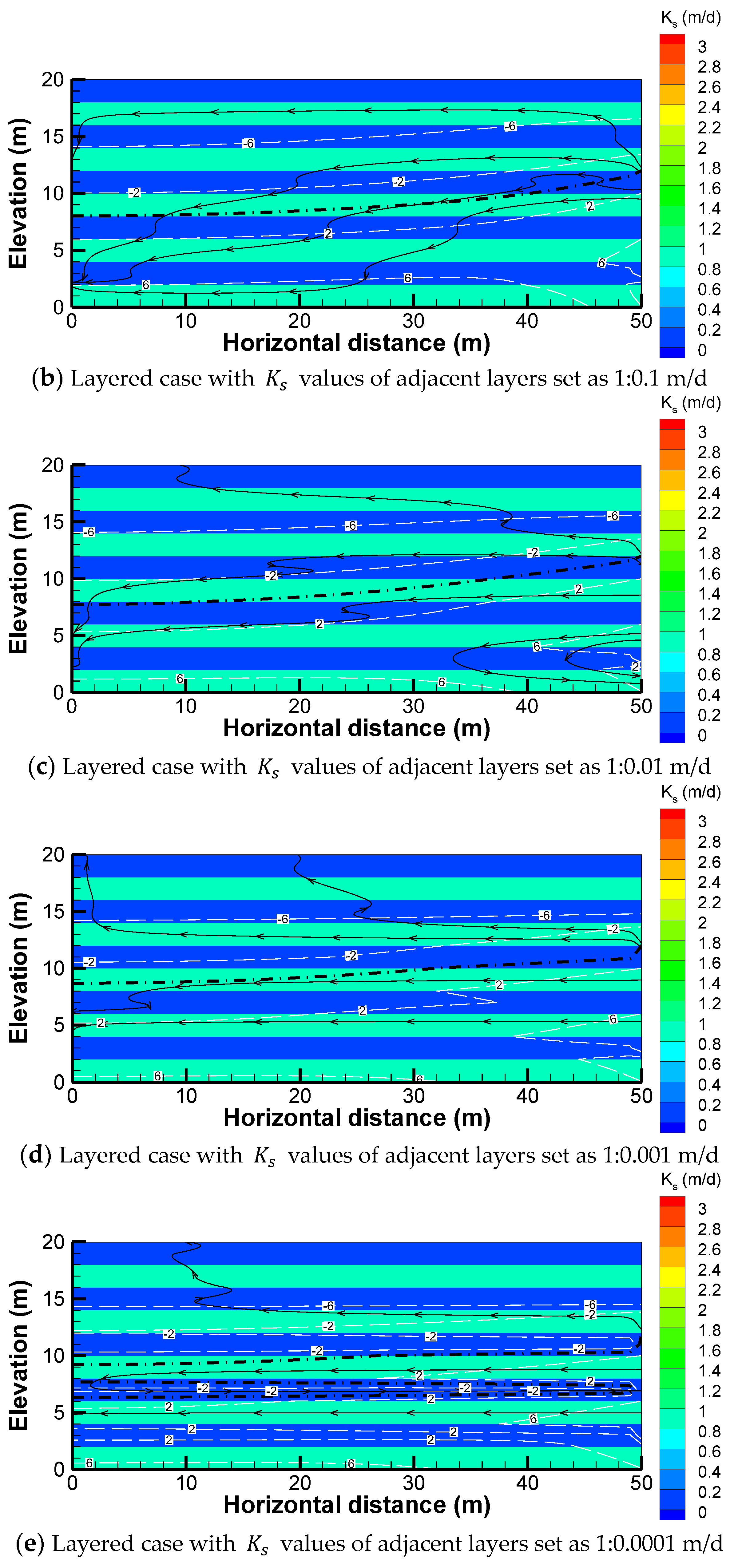
3.1. Deterministic Analysis of Layered Foundation

To illustrate the effect of the layered structure of foundations on the groundwater responses subjected to water level fluctuation in a reservoir, we generated four layered foundation profiles with the layer sizes fixed as 50 m × 2 m. The saturated hydraulic conductivity $K_s$ values of the adjacent layers are 1:0.1, 1:0.01, 1:0.001, and 1:0.0001 (m/d), respectively, representing different degrees of layering. As a comparison, a homogeneous case with a $K_s$ value of 1 m/d was also generated. These five cases were subsequently under a transient groundwater response analysis subjected to 3 days’ water level fluctuation in a reservoir with $T=0.5$ day. The spatial distributions of the $K_s$ fields, phreatic surface (denoted by the black dot dash line), pressure head $p$ (denoted by the white dashed lines with labels), and streamlines (denoted by the black solid line with arrows) of the five cases at $t=3$ days are presented in Figure 2. As can be seen in Figure 2, the homogeneous case has the largest groundwater responses in the foundation from the reservoir water level fluctuation due to its large $K_s$. The pressure head isolines and the phreatic surface are mostly horizontal. The pressure head decreases from lower elevation to higher elevation, and the phreatic surface at the distal end of the foundation is around 9.5 m of elevation and is the highest among the five cases. The streamlines are from the reservoir to the distal end of foundation with long smooth segments. For layered cases, due to layers with low $K_s$ values, the pressure head isolines become complex, which are tortuous and repeated. The phreatic surface at the distal end becomes lower than that in the homogeneous case, and it gradually rises again when the differences between the $K_s$ values of the adjacent layers increase. The streamlines stay mostly in the high $K_s$ layer and pass through the low $K_s$ layer with relatively shorter paths. These results demonstrate that the foundation structures have significant impacts on the groundwater response to the reservoir water level fluctuations.

Figure 3 plots the contour maps of the pressure head $p$ of the layered foundation with $K_s$ values of adjacent layers set as 1:0.0001 m/d at four selected time steps: t = 0.51, 1.01, 2.01, and 3 days, respectively. As can be seen from these figures, the groundwater flows in the foundation mainly through high $K_s$ layers. It gradually flows into the foundation and accumulates at the distal end, and the groundwater transported by the high $K_s$ layers is reduced as the elevation increases. Note that although the effect from the reservoir water level fluctuation decreases near the top of the foundation, this does not mean that the groundwater responses have little influence on the foundation and the structures built on it. The transportation and accumulation of groundwater lead to the increase in the pressure head at parts of the foundation; this may further result in differential deformation. For comparison, the contour maps of the pressure head $p$ of the homogeneous case at the four selected time steps are plotted in Figure 4. As expected, the pressure head decreases evenly with elevation, and the horizontal differences are smaller compared to those of the layered cases. The results from the homogeneous case with $K_s=1 \mathrm{m}/\mathrm{d}$ can be viewed as the average of all results of the layered cases with their spatial mean $K_s$, denoted as ${\mu }_{K_s}$, equaling 1 m/d.

To provide a better illustration, we plotted the pressure heads $p$ along the cross-section 1-1′ at $t=3$ days for the five cases in Figure 5. The pressure head of the homogenous case decreases linearly from 10 m to −10 m as the elevation increases. The pressure head of the layered case, due to the existence of low $K_s$ layers, becomes tortuous and smaller than that of the homogeneous case. The pressure heads of high $K_s$ layers are larger than those of their adjacent low $K_s$ layers. As the discrepancy between the $K_s$ values of the adjacent layers increases, the pressure head at the high $K_s$ layer increases, and that at the low $K_s$ layer decreases, and thus, the difference between the pressure head of the high $K_s$ layer and the low $K_s$ layer increases. The pressure head at the high $K_s$ layer could become larger than that at the same elevation in the homogeneous case.

3.2. Probabilistic Analysis of Layered Foundation

In reality, the layers in the layered foundation are not perfectly extended, their thicknesses are not uniform, and they are not evenly distributed. These lead to the need for probabilistic descriptions of the $K_s$ field of the layered structure of the foundation.

3.2.1. Probabilistically Description of Layered Structure

Generally, for the layered foundation, the mean of the saturated hydraulic conductivity, ${\mu }_{K_s}$, describes the overall permeability level of the layers in the foundation. The variance of saturated hydraulic conductivity, ${\sigma }_{K_s}^2$, describes the contrast between different layers. The horizontal and vertical correlation scales of saturated hydraulic conductivity, ${\lambda }_h$ and ${\lambda }_v$, describe the average sizes of layers in horizontal and vertical directions, respectively.

Six cases listed in

Table 2. Study cases.

Case No.	${\mathit{\sigma }}_{\mathit{l}\mathit{n}{\mathit{K}}_{\mathit{s}}}^2$	${\mathit{\lambda }}_{\mathit{h}}$	${\mathit{\lambda }}_{\mathit{v}}$	$\mathit{T}$
1	1	50	2	0.5
2	4	50	2	0.5
3	1	25	2	0.5
4	1	5	2	0.5
5	1	50	4	0.5
6	1	50	2	0.3

are used to further probabilistically investigate the groundwater responses of a layered foundation subjected to water level fluctuation in a reservoir while considering the spatial variability of the parameters. Specifically, cases 1 and 2 focus on the effects of variance in the logarithm of the saturated hydraulic conductivity, ${\sigma }_{ln{K}_s}^2$; cases 1, 3, and 4 focus on the effects of the horizontal correlation scale of saturated hydraulic conductivity, ${\lambda }_h$; cases 1 and 5 focus on the effects of the vertical correlation scale, ${\lambda }_v$; and cases 1 and 6 focus on the effects of the one-way time consumption of fluctuations, $T$.

To demonstrate the effectiveness of the probabilistic description method, one realization to each case is generated for cases 1 to 5. These realizations are generated using the Karhunen–Loève (K-L) expansion [22,23,24,25,26,27,28,29]. The spatial distributions of $K_s$ fields, phreatic surface (denoted by the black dot dash line), pressure head $p$ (denoted by the white dashed lines with labels), and streamlines (denoted by the black solid line with arrows) of the five cases at $t=3$ days are presented in Figure 6. These results, again, demonstrate the importance of spatial variability in the structure characteristics of layered foundations regarding the groundwater responses subjected to water level fluctuation in a reservoir. As indicated in Figure 6, the location and shape of the phreatic surface, the pressure head profiles, and the streamlines of the five cases are different to each other. With the decrease in ${\lambda }_h$ or ${\lambda }_v$, the streamlines become relatively fluctuated. This is due to the spatially rough variation of $K_s$.

3.2.2. Uncertainty Analysis of Layered Foundation

Since the variability in the layered structure of the foundation results in variation in the groundwater responses of the foundation, the uncertainty in groundwater flow should be estimated for a reliable analysis. Substituting the statistics in Table 2 into the first-order moment approach [17,18,19] yields the standard deviation of $p$, denoted as ${\sigma }_p$, at each location of the foundation, representing the distribution of the uncertainty of $p$ in the foundation. The ${\sigma }_p$ fields of foundation subjected to reservoir water level fluctuation at $t=3$ days for the six cases are shown in Figure 7. For a better comparison, we plotted the ${\sigma }_p$ profiles along the cross-section 1-1′ in Figure 8.

As shown in these figures, the regions with relatively large uncertainties in the foundation are those around the initial water level at the reservoir side, and those at the distal end away from the reservoir. The comparison of case 1 and case 2 indicates that a larger ${\sigma }_{ln{K}_s}^2$ leads to larger uncertainty in $p$. This is to be expected. The comparison of cases 1, 3, and 4 indicates that a smaller ${\lambda }_h$ leads to smaller uncertainty in $p$. This implies that the defects of the layer improve the groundwater exchange and ease the difference between different realizations; thus, the ${\sigma }_p$ value decreases. The comparison of case 1 and case 5 indicates that a larger ${\lambda }_v$ leads to larger uncertainty in $p$ at most parts, but it leads to smaller uncertainty in $p$ near the initial water level at the reservoir side. This may be due to the fact that a larger ${\lambda }_v$ value increases the opportunity for reservoir water to flow in, but it decreases the opportunity for groundwater exchange. Finally, the comparison of case 1 and case 6 indicates that a smaller $T$ leads to smaller uncertainty in $p$. This implies that a faster reservoir level scheduling would reduce the uncertainty of groundwater responses; this may be because a smaller $T$ value means there is less time for reservoir water to flow in, and hence, less amount of water flows into the foundation during the fluctuation cycle.

Figure 9 quantifies the influence of different factors (${\sigma }_{ln{K}_s}^2$, ${\lambda }_h$, ${\lambda }_v$, and $T$) on ${\sigma }_p$ in the foundation. The influences of these four factors are expressed as the average change in the ${\sigma }_p$ value along the cross-section 1-1′ versus the increase percentage of each factor. As indicated in Figure 9, the four factors all have positive correlations with ${\sigma }_p$. In addition, ${\sigma }_{ln{K}_s}^2$ has the largest impact on ${\sigma }_p$ in the foundation, ${\lambda }_v$ has the second largest impact, and ${\lambda }_h$ has the smallest impact. That is, larger ${\sigma }_{ln{K}_s}^2$, ${\lambda }_v$, $T$, and ${\lambda }_h$ values would lead to larger uncertainty in the estimation of groundwater responses in the foundation.

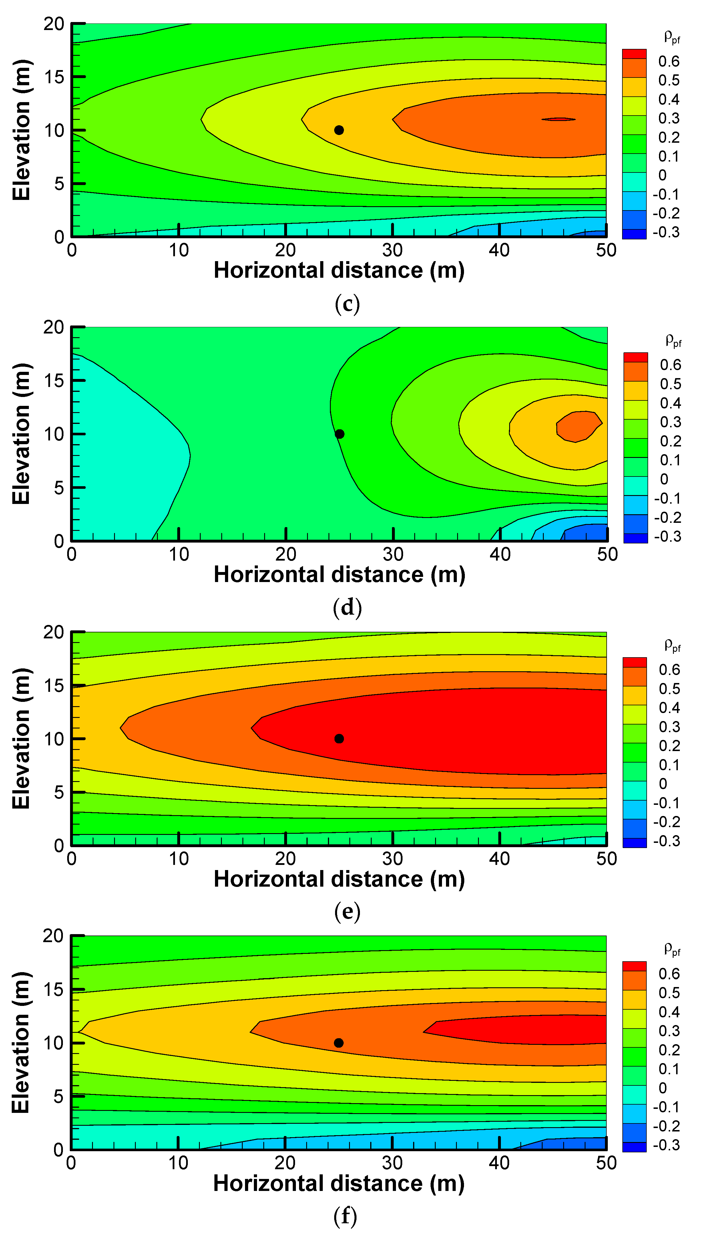
3.2.3. Cross-Correlation Analysis

To further reveal the spatial relationship between the pressure head $p$ at one location and $K_s$ at each location in the foundation, we conduct a cross-correlation analysis in this section. The cross-correlation analysis considers the sensitivity, the effects of magnitudes of heterogeneity (variance) between layers, and the layered structure of the foundation (correlation scales) (see Cai et al. [30]). The cross-correlation fields of $p$ at a selected location (horizontal distance = 25 m; elevation = 10 m) to $\ln K_S$ at each location in the foundation subjected to reservoir water level fluctuation at $t=3$ days for the six cases are plotted in Figure 10. From Figure 10, we see the $p$ value at any one location is positively correlated with the $K_s$ values around the highest water level at the reservoir side, and it is negatively correlated with the $K_s$ values around the initial water level at the reservoir side. In addition, the changes in ${\lambda }_h$ and ${\lambda }_v$ have significant impacts on the cross-correlation maps, and the change in ${\sigma }_{ln{K}_s}^2$ has little effect on the cross-correlation maps. The decrease in $T$ increases the absolute value of the cross-correlation. As expected, a foundation with small $K_s$ values around the initial water level at the reservoir side and large $K_s$ values around the highest water level at the reservoir side may produce a larger $p$ value in the foundation.

4. Conclusions

The groundwater response to reservoir water level fluctuations highly depends on the foundation of soil structures. This paper investigates the effect of variability in the layered structure of a foundation on the distribution of the pressure head in a foundation subjected to water level fluctuation in a reservoir. The variability in the layered structure of a foundation is described by the spatial variability of saturated hydraulic conductivity. With the aid of the random field theory, Karhunen–Loève (K-L) expansion, first-order moment approach, and cross-correlation analysis, the way the groundwater changes with the water level variation in a reservoir is revealed.

A deterministic analysis demonstrates that foundation structures have significant impacts on the groundwater response to reservoir water level fluctuations. The reservoir water flows into the foundation mainly through high $K_s$ layers and is gradually accumulated at the distal end away from the reservoir. The groundwater transported by the high $K_s$ layers is reduced as the elevation increases. In addition, the pressure heads of high $K_s$ layers are larger than those of their adjacent low $K_s$ layers. As the discrepancy between the $K_s$ values of adjacent layers increases, the difference between the pressure head of the high $K_s$ layer and the low $K_s$ layer increases. The pressure head at a high $K_s$ layer could even become larger than that at the same elevation in the homogeneous case.

A probabilistic analysis further indicates that the regions with relatively large uncertainties in the foundation are those around the initial water level at the reservoir side and those at the distal end away from the reservoir. In addition, a larger ${\sigma }_{ln{K}_s}^2$, a larger ${\lambda }_h$, a larger ${\lambda }_v$, and a larger $T$ lead to larger uncertainty in the pressure head. Moreover, the four factors (${\sigma }_{ln{K}_s}^2$, ${\lambda }_h$, ${\lambda }_v$, and $T$) all have positive correlations with ${\sigma }_p$. ${\sigma }_{ln{K}_s}^2$ has the largest impact on ${\sigma }_p$ in the foundation, ${\lambda }_v$ has the second largest impact, and ${\lambda }_h$ has the smallest impact. The uncertainty in $p$ plays a critical role in the evaluations of the stability and performance of foundations. Further investigation or monitoring measures should be implemented to the location of the large-uncertainty zone to reduce the uncertainty. As a result, any unfavorable conditions can be detected immediately before it is too late.

Lastly, a cross-correlation analysis indicates that the pressure head $p$ at any one location is positively correlated with the $K_s$ values around the highest water level at the reservoir side and is negatively correlated with the $K_s$ values around the initial water level at the reservoir side. In addition, the changes in ${\lambda }_h$ and ${\lambda }_v$ have significant impacts on the cross-correlation maps. The decrease in $T$ increases the absolute value of the cross-correlation. As expected, a foundation with small $K_s$ values around the initial water level at the reservoir side and large $K_s$ values around the highest water level at the reservoir side may produce a larger $p$ value in the foundation. This is unfavorable to the stability of foundations and deserves special attention.

Although the spatial variabilities in the saturated hydraulic conductivity $K_s$ of foundations with layer structures are merely considered, these results yield useful insights into the effect of variability in the layered structure of a foundation on the distribution of the pressure head in a foundation subjected to water level fluctuation in a reservoir. Further focus could be placed on the spatial variabilities of other parameters such as the specific storage $S_s$ and the MVG model parameters, $\alpha$ and $n$, which have been shown to have strong spatial variability [31].

References

1. Alencar, A.; Galindo, R.; Melentijevic, S. Influence of the Groundwater Level on the Bearing Capacity of Shallow Foundations on the Rock Mass. Bull. Eng. Geol. Environ. 2021, 80, 6769–6779. [Google Scholar] [CrossRef]
2. Ausilio, E.; Conte, E. Influence of Groundwater on the Bearing Capacity of Shallow Foundations. Can. Geotech. J. 2005, 42, 663–672. [Google Scholar] [CrossRef]
3. Chen, W.; Xia, W.; Zhang, S.; Wang, E. Study on the Influence of Groundwater Variation on the Bearing Capacity of Sandy Shallow Foundation. Appl. Sci. 2023, 13, 473. [Google Scholar] [CrossRef]
4. Chen, J.; Huang, Y.; Yang, Y.; Wang, J. Evaluation of the Influence of Jiangxiang Reservoir Immersion on Corp and Residential Areas. Geofluids 2018, 2018, 9720970. [Google Scholar] [CrossRef]
5. Ahmed, A.A. Stochastic Analysis of Free Surface Flow through Earth Dams. Comput. Geotech. 2009, 36, 1186–1190. [Google Scholar] [CrossRef]
6. Cho, S.E. Probabilistic Analysis of Seepage That Considers the Spatial Variability of Permeability for an Embankment on Soil Foundation. Eng. Geol. 2012, 133–134, 30–39. [Google Scholar] [CrossRef]
7. Rulon, J.J.; Freeze, R.A. Multiple Seepage Faces on Layered Slopes and Their Implications for Slope-Stability Analysis. Can. Geotech. J. 1985, 22, 347–356. [Google Scholar] [CrossRef]
8. Ng, C.W.W.; Wang, B.; Tung, Y.K. Three-Dimensional Numerical Investigations of Groundwater Responses in an Unsaturated Slope Subjected to Various Rainfall Patterns. Can. Geotech. J. 2001, 38, 1049–1062. [Google Scholar] [CrossRef]
9. Srivastava, A.; Babu, G.L.L.S.; Haldar, S. Influence of Spatial Variability of Permeability Property on Steady State Seepage Flow and Slope Stability Analysis. Eng. Geol. 2010, 110, 93–101. [Google Scholar] [CrossRef]
10. Santoso, A.M.; Phoon, K.-K.; Quek, S.-T. Effects of Soil Spatial Variability on Rainfall-Induced Landslides. Comput. Struct. 2011, 89, 893–900. [Google Scholar] [CrossRef]
11. Griffiths, D.V.; Fenton, G.A.; Manoharan, N. Undrained Bearing Capacity of Two-Strip Footings on Spatially Random Soil. Int. J. Geomech. 2006, 6, 421–427. [Google Scholar] [CrossRef]
12. Griffiths, D.V.; Fenton, G.A.; Manoharan, N. Bearing Capacity of Rough Rigid Strip Footing on Cohesive Soil: Probabilistic Study. J. Geotech. Geoenviron. Eng. 2002, 128, 743–755. [Google Scholar] [CrossRef]
13. Li, J.; Tian, Y.; Cassidy, M.J. Failure Mechanism and Bearing Capacity of Footings Buried at Various Depths in Spatially Random Soil. J. Geotech. Geoenviron. Eng. 2015, 141, 04014099. [Google Scholar] [CrossRef]
14. Fenton, G.A.; Griffiths, D.V. Bearing Capacity of Spatially Random Soils. In Proceedings of the 8th ASCE Joint Specialty Conference on Probabilistic Mechanics and Structural Reliability, Notre Dame, IN, USA, 24–26 July 2000; University of Notre Dame: Notre Dame, IN, USA, 2000; Volume 40, pp. 1–6. [Google Scholar]
15. Griffiths, D.V.; Fenton, G.A. Bearing Capacity of Spatially Random Soil: The Undrained Clay Prandtl Problem Revisited. Géotechnique 2001, 51, 351–359. [Google Scholar] [CrossRef]
16. Mualem, Y. A new model for predicting the hydraulic conductivity of unsaturated porous media. Water Resour. Res. 1976, 12, 513–522. [Google Scholar] [CrossRef]
17. Van Genuchten, M.T. A closed-form equation for predicting the hydraulic con-ductivity of unsaturated soils. Soil Sci. Soc. Am. J. 1980, 44, 892. [Google Scholar] [CrossRef]
18. Yeh, T.J.; Srivastava, R.; Guzman, A.; Harter, T. A Numerical Model for Water Flow and Chemical Transport in Variably Saturated Porous Media. Ground Water 1993, 31, 634–644. [Google Scholar] [CrossRef]
19. Tang, R.-X.; Cai, J.-S.; Yeh, T.-C.J. Two-Dimensional Probabilistic Infiltration Analysis in a Hillslope Using First-Order Moment Approach. Groundwater 2019, 57, 226–237. [Google Scholar] [CrossRef]
20. Khaleel, R.; Freeman, E.J. Variability and Scaling of Hydraulic Properties for 200 Area Soils, Hanford Site; Rep. WHC-EP-0883; Westinghouse Hanford Co.: Richland, WA, USA, 1995. [Google Scholar]
21. Yeh, T.-C.; Khaleel, R.; Carroll, K.C. Flow through Heterogeneous Geologic Media; Cambridge University Press: New York, NY, USA, 2015; ISBN 9781107076136. [Google Scholar]
22. Huang, S.P. Simulation of Random Processes Using Karhunen-Loeve Expansion. Doctoral Dissertation, National University of Singapore, Singapore, 2001. [Google Scholar]
23. Cho, S.E. Probabilistic Stability Analysis of Rainfall-Induced Landslides Considering Spatial Variability of Permeability. Eng. Geol. 2014, 171, 11–20. [Google Scholar] [CrossRef]
24. Ali, A.; Huang, J.; Lyamin, A.V.; Sloan, S.W.; Griffiths, D.V.; Cassidy, M.J.; Li, J.H. Simplified Quantitative Risk Assessment of Rainfall-Induced Landslides Modelled by Infinite Slopes. Eng. Geol. 2014, 179, 102–116. [Google Scholar] [CrossRef]
25. Jiang, S.-H.; Li, D.-Q.; Cao, Z.-J.; Zhou, C.-B.; Phoon, K.-K. Efficient System Reliability Analysis of Slope Stability in Spatially Variable Soils Using Monte Carlo Simulation. J. Geotech. Geoenviron. Eng. 2015, 141, 04014096. [Google Scholar] [CrossRef]
26. Huang, J.; Griffiths, D.V. Determining an Appropriate Finite Element Size for Modelling the Strength of Undrained Random Soils. Comput. Geotech. 2015, 69, 506–513. [Google Scholar] [CrossRef]
27. Cai, J.-S.; Yeh, T.J.; Yan, E.-C.; Hao, Y.-H.; Huang, S.; Wen, J.-C. Uncertainty of Rainfall-Induced Landslides Considering Spatial Variability of Parameters. Comput. Geotech. 2017, 87, 149–162. [Google Scholar] [CrossRef]
28. Ghanem, R.G.; Spanos, P.D. Stochastic Finite Elements: A Spectral Approach; Springer: New York, NY, USA, 1991; ISBN 978-1-4612-3094-6. [Google Scholar]
29. Cai, J.-S.; Yeh, T.-C.J.; Yan, E.-C.; Tang, R.-X.; Wen, J.-C.; Huang, S.-Y. An Adaptive Sampling Approach to Reduce Uncertainty in Slope Stability Analysis. Landslides 2018, 15, 1193–1204. [Google Scholar] [CrossRef]
30. Cai, J.-S.; Yan, E.-C.; Yeh, T.J.; Zha, Y.-Y. Sampling Schemes for Hillslope Hydrologic Processes and Stability Analysis Based on Cross-Correlation Analysis. Hydrol. Process. 2017, 31, 1301–1313. [Google Scholar] [CrossRef]
31. Yeh, T.J.; Gelhar, L.W.; Gutjahr, A.L. Stochastic Analysis of Unsaturated Flow in Heterogeneous Soils: 1. Statistically Isotropic Media. Water Resour. Res. 1985, 21, 447–456. [Google Scholar] [CrossRef]
Figure 1. The model of the foundation subjected to reservoir water level fluctuation.
Water 16 00081 g001
Figure 2. Spatial distributions of K s fields, phreatic surface (denoted by the black dot dash line), pressure head p (denoted by the white dashed lines with labels), and streamlines (denoted by the black solid line with arrows) of cases of layered foundations subjected to reservoir water level fluctuation at t = 3 days.
Water 16 00081 g002aWater 16 00081 g002b
Figure 3. Spatial distributions of pressure head p of the layered foundation with K s values of adjacent layers set as 1:0.0001 m/d at four selected time steps.
Water 16 00081 g003
Figure 4. Spatial distributions of pressure head p of the homogeneous foundation at four selected time steps.
Water 16 00081 g004
Figure 5. Pressure head p of realizations of layered foundations along cross-section 1-1′ at t = 3 days.
Water 16 00081 g005
Figure 6. Spatial distributions of K s fields, phreatic surface (denoted by the black dot dash line), pressure head p (denoted by the white dashed lines with labels), and streamlines (denoted by the black solid line with arrows) at t = 3 days for realizations of cases 1 to 5. (a) Case 1 (see Table 2); (b) Case 2; (c) Case 3; (d) Case 4; (e) Case 5.
Water 16 00081 g006aWater 16 00081 g006b
Figure 7. Standard deviations of pressure heads σ p of foundation subjected to reservoir water level fluctuation at t = 3 days. (a) Case 1 (see Table 2); (b) Case 2; (c) Case 3; (d) Case 4; (e) Case 5; (f) Case 6.
Water 16 00081 g007aWater 16 00081 g007b
Figure 8. Standard deviations of pressure heads σ p of foundation at t = 3 days along cross-section 1-1′.
Water 16 00081 g008
Figure 9. Average changes in σ p along the cross-section 1-1′ at t = 3 days with increase percentage of different factors.
Water 16 00081 g009
Figure 10. Cross-correlation of pressure heads p to f = ln K s in the foundation subjected to reservoir water level fluctuation at t = 3 days. (a) Case 1 (see Table 2); (b) Case 2; (c) Case 3; (d) Case 4; (e) Case 5; (f) Case 6.
Water 16 00081 g010aWater 16 00081 g010b