
Research on Extension Evaluation Method of Mudslide Hazard Based on Analytic Hierarchy Process–Criteria Importance through Intercriteria Correlation Combination Assignment of Game Theory Ideas

 ,
,
Abstract
:1. Introduction
2. Study Area
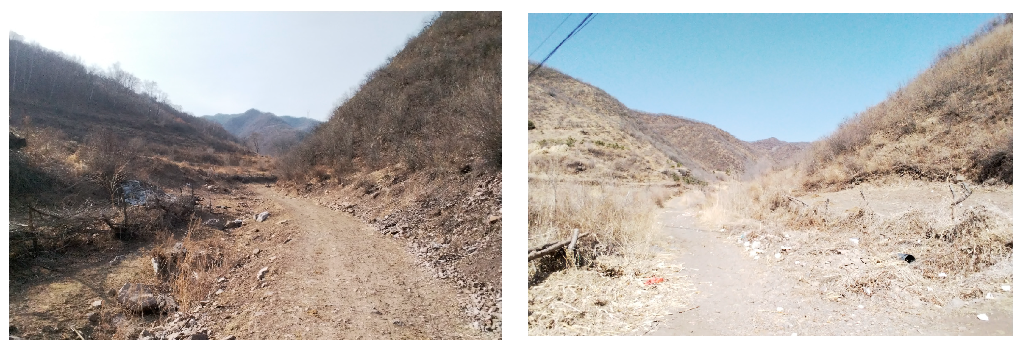
2.1. Overview of the Evaluation Area
2.2. Determination of Debris Flow Hazard Evaluation Index
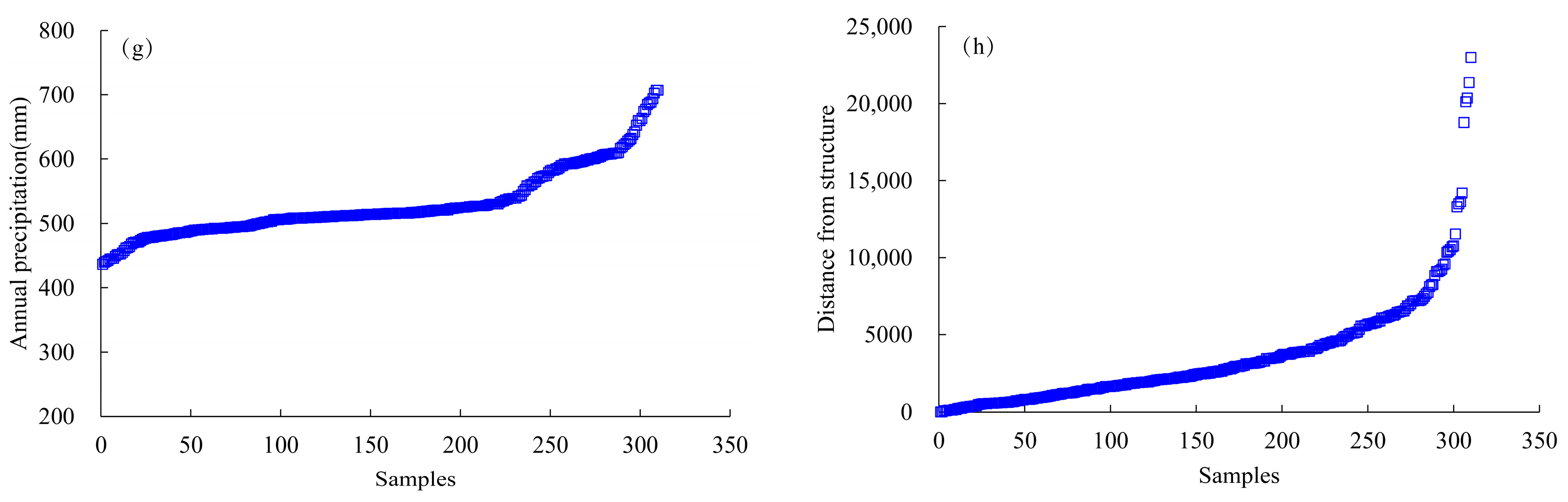
2.3. Data Sources
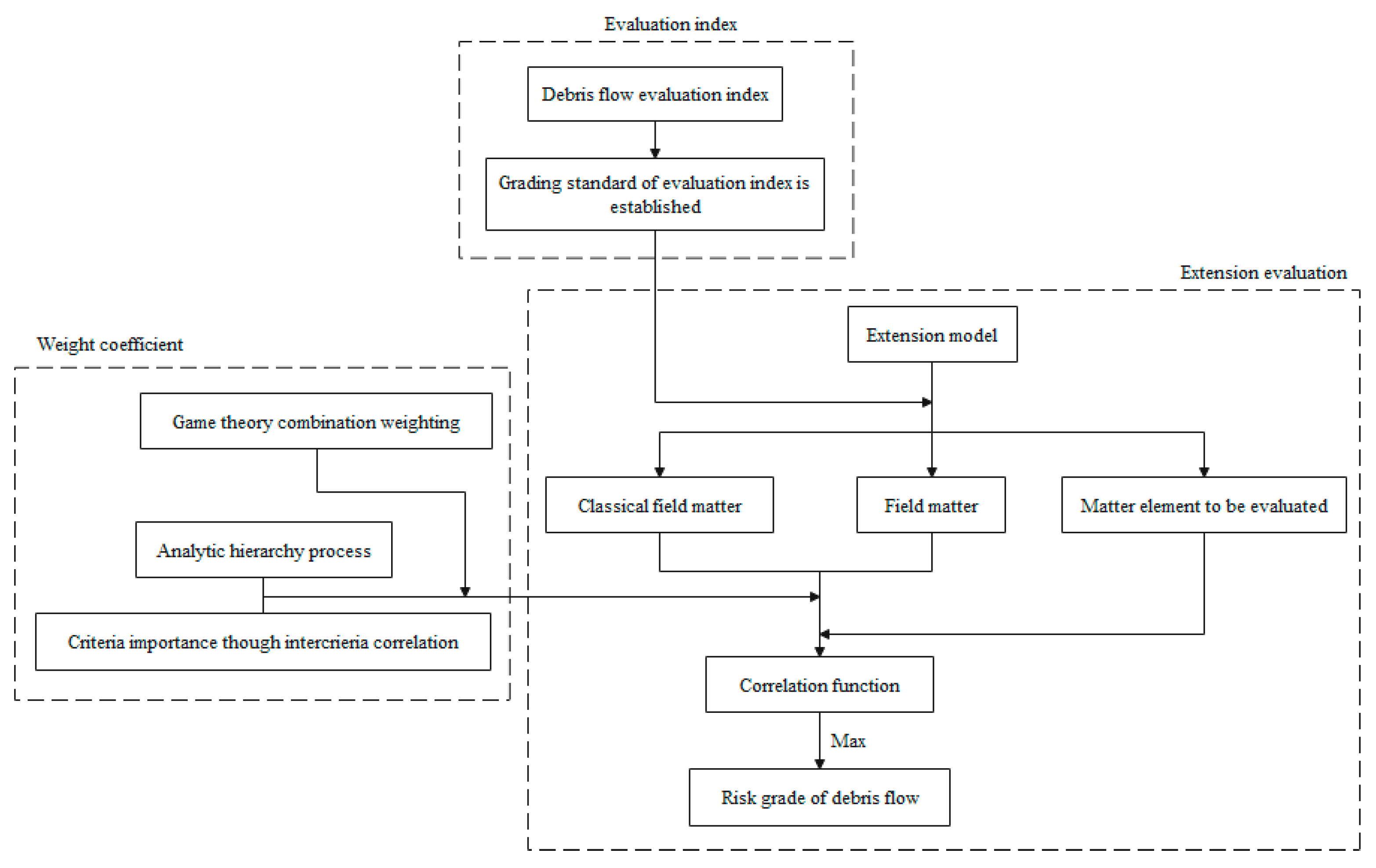
3. Methods
3.1. Extensional Matter Element Model
3.2. Weighting Factor
3.3. Evaluation Index Level and Grading
4. Results
4.1. Topological Model
4.2. Weighting Coefficient
4.3. Matter-Element Model to Be Evaluated
5. Discussion
5.1. Evaluation Results
5.2. Evaluation Method Optimization
5.3. Application of Evaluation Methods
6. Conclusions
Author Contributions
Funding
Data Availability Statement
Conflicts of Interest
References
- Kang, Z.; Li, C.; Ma, A.; Luo, J. Study on Debris Flow in China; Science Press: Beijing, China, 2004; pp. 1–15. [Google Scholar]
- Sebastián, F.D.; Valérie, B.; Noelia, C. The twin catastrophic flows occurred in 2014 at Ambato Range (28°09′–28°20′ S), Catamarca Province, Northwest Argentina. J. S. Am. Earth Sci. 2021, 106, 103086. [Google Scholar]
- Chao, K.; Dave, C. Investigation of erosion characteristics of debris flow based on historical cases. Eng. Geol. 2022, 306, 106767. [Google Scholar]
- Gisonni, C. Debris flow: Mechanics, prediction and countermeasures. J. Hydraul. Res. 2008, 46, 144. [Google Scholar] [CrossRef]
- He, Z. Development characteristics of debris flow and its influence on migration site. BioTechnol. Indian J. 2014, 10, 8818–8821. [Google Scholar]
- Okubo, S.; Ikeya, H.; Ishikawa, Y.; Yamada, T. Development of new methods for countermeasures against debris flows. Recent Dev. Debris Flows 2007, 64, 166–185. [Google Scholar]
- Tang, C.; van Asch, T.W.; Chang, M.; Chen, G.Q.; Zhao, X.H.; Huang, X.C. Catastrophic debris flows on 13 August 2010 in the Qingping area, southwestern China: The combined effects of a strong earthquake and subsequent rainstorms. Geomorphology 2012, 139, 559–576. [Google Scholar] [CrossRef]
- Breien, H.; De Blasio, F.V.; Elverhøi, A.; Høeg, K. Erosion and morphology of a debris flow caused by a glacial lake outburst flood, Western Norway. Landslides 2008, 5, 271–280. [Google Scholar] [CrossRef]
- Fiorillo, F.; Wilsion, R.C. Rainfall induced debris flows in pyroclastic deposits, Campania (Southern Italy). Eng. Geol. 2004, 75, 263–289. [Google Scholar] [CrossRef]
- Shang, Y. Geological and Geomorphologic Disasters and Disaster Prevention and Reduction in Hebei Province. J. Catastrophol. 1999, 14, 33–38. [Google Scholar]
- Bentivenga, M.; Bellanova, J.; Calamita, G.; Capece, A.; Cavalcante, F.; Gueguen, E.; Guglielmi, P.; Murgante, B.; Palladino, G.; Perrone, A.; et al. Geomorphological and geophysical surveys with InSAR analysis applied to the Picerno earth flow (southern Apennines, Italy). Landslides 2021, 18, 471–483. [Google Scholar] [CrossRef]
- Carolin, K.; Patrick, O.; Jasper, M.; Claudio, F.S.; Christoph, M.; Michael, S.; Michael, K. A 4000-year debris flow record based on amphibious investigations of fan delta activity in Plansee (Austria, Eastern Alps). Earth Surf. Dyn. 2021, 9, 1481–1503. [Google Scholar]
- Zhou, G.; Lyu, L.; Xu, M.; Ma, C.; Wang, Y.; Wang, Y.; Wang, Z.; Stoffel, M. Assessment of check dams and afforestation in mitigating debris flows based on dendrogeomorphic reconstructions, field surveys and semi-empirical models. Catena 2023, 232, 107434. [Google Scholar] [CrossRef]
- Teemu, H.; Peter, F.; Philip, S.; Philipp, R.; Ansgar, W.; Andreas, V.; Frieder, E. Multi-Methodological Investigation of the Biersdorf Hillslope Debris Flow (Rheinland-Pfalz, Germany) Associated to the Torrential Rainfall Event of 14 July 2021. Geosciences 2022, 12, 245. [Google Scholar]
- Seph, B.Y.; Gi, K.M.; Han, P.K.; Keun, O.T.; Hyun, S.J. Development of the Damage Investigation Item to Debris Flow using the Delphi Method. J. Korean Soc. Saf. 2016, 31, 41–48. [Google Scholar]
- Nejc, B.; Jošt, S.; Matej, M.; Timotej, J.; Jernej, J.; Tina, P.; Matjaž, M. Investigation of potential debris flows above the Koroška Bela settlement, NW Slovenia, from hydro-technical and conceptual design perspectives. Landslides 2021, 18, 3891–3906. [Google Scholar]
- Peng, B.; Xiao, X.; Zhao, B.; Li, H. Application of digital twins in high precision geological hazard survey and prevention in Beijing. Int. Arch. Photogramm. Remote Sens. Spat. Inf. Sci. 2022, XLVIII-3/W1-2022, 39–44. [Google Scholar] [CrossRef]
- Chalk, C.M.; Peakall, J.; Keevil, G.; Fuentes, R. Spatial and temporal evolution of an experimental debris flow, exhibiting coupled fluid and particulate phases. Acta Geotech. 2021, 17, 965–979. [Google Scholar] [CrossRef]
- Baselt, I.; de Oliveira, G.Q.; Fischer, J.-T.; Pudasaini, S.P. Evolution of stony debris flows in laboratory experiments. Geomorphology 2021, 372, 107431. [Google Scholar] [CrossRef]
- van Asch, T.W.J.; Yu, B.; Hu, W. The Development of a 1-D Integrated Hydro-Mechanical Model Based on Flume Tests to Unravel Different Hydrological Triggering Processes of Debris Flows. Water 2018, 10, 950. [Google Scholar] [CrossRef]
- Haruka, T.; Yoshinori, S.; Norifumi, H.; Christopher, G.; Yuichi, S. Multi-decadal changes in the relationships between rainfall characteristics and debris-flow occurrences in response to gully evolution after the 1990–1995 Mount Unzen eruptions. Earth Surf. Process. Landf. 2021, 46, 2141–2162. [Google Scholar]
- Rickenmann, D. Debris-Flow Hazard Assessment and Methods Applied in Engineering Practice. Int. J. Eros. Control Eng. 2016, 9, 80–90. [Google Scholar] [CrossRef]
- Kim, S.; Lee, H.-J. Assessment of Risk Due to Debris Flow and Its Application to a Marine Environment. Mar. Georesour. Geotechnol. 2015, 33, 572–578. [Google Scholar] [CrossRef]
- Roberti, G.; Friele, P.; van Wyk de Vries, B.; Ward, B.; Clague, J.J.; Perotti, L.; Giardino, M. Rheological evolution of the Mount Meager 2010 debris avalanche, southwestern British Columbia. Geosphere 2017, 13, 369–390. [Google Scholar] [CrossRef]
- Eldeen, M.T. Predisaster physical planning:intergration of disasterrisk analys is into physical planning acase study in Tunisia. Disasters 1980, 4, 211–222. [Google Scholar] [CrossRef] [PubMed]
- Hollingsworth, R.; Kovacs, G.S. Soil Slumps and Debris Flows: Prediction and Protection. Environ. Eng. Geosci. 1981, xviii, 17–28. [Google Scholar] [CrossRef]
- Ohmori, H.; Hirano, M. Magnitude frequency and geomorphological significance of rocky debris flows, landcreep and the collapse of steep slopes. Z. Fur Geomorphol. 1988, 67, 55–65. [Google Scholar]
- Carrara, A.; Cardinali, M.; Detti, R.; Guzzetti, F.; Pasqui, V.; Reichenbach, P. GIS techniques and statistical models in evaluating landslide hazard. Earth Surf. Process. Landf. 1991, 16, 427–445. [Google Scholar] [CrossRef]
- Carrara, A. Uncertainty in Assessing Landslide Hazard and Risk. In Prediction and Perception of Natural Hazards; Springer: Berlin/Heidelberg, Germany, 1992; pp. 101–109. [Google Scholar]
- Ran, L.M.; Myoung, C.J.; Sic, Y.H. Quantitative Risk Analysis of Debris Flow Disasters in Urban Area Using Geographic Information System. Sens. Mater. 2020, 32, 4573–4586. [Google Scholar]
- Pallàs, R.; Vilaplana, J.M.; Guinau, M.; Falgàs, E.; Alemany, X.; Muñoz, A. A pragmatic approach to debris flow hazard mapping in areas affected by Hurricane Mitch: Example from NW Nicaragua. Eng. Geol. 2003, 72, 57–72. [Google Scholar] [CrossRef]
- Kim, H.-S.; Chung, C.-K.; Kim, S.-R.; Kim, K.-S. A GIS-Based Framework for Real-Time Debris-Flow Hazard Assessment for Expressways in Korea. Int. J. Disaster Risk Sci. 2016, 7, 293–311. [Google Scholar] [CrossRef]
- Joong, R.H.; Hwan, S.J.; Seok, S.H.; Hong, K.G.; Woo, L.S. A Model for Evaluation of Debris Flow Risk in a Watershed. J. Korean Soc. Hazard Mitig. 2012, 12, 67–76. [Google Scholar]
- Gomez, C.; Purdie, H. Point cloud technology and 2D computational flow dynamic modeling for rapid hazards and disaster risk appraisal on Yellow Creek fan, Southern Alps of New Zealand. Prog. Earth Planet. Sci. 2018, 5, 50. [Google Scholar] [CrossRef]
- Monia, C.; Valeria, M.; Vania, M.; Nicola, S.; Enrico, M. Rockfall and Debris Flow Hazard Assessment in the SW Escarpment of Montagna del Morrone Ridge (Abruzzo, Central Italy). Water 2020, 12, 1206. [Google Scholar]
- Horton, A.J.; Hales, T.C.; Ouyang, C.; Fan, X. Identifying post-earthquake debris flow hazard using Massflow. Eng. Geol. 2019, 258, 105134. [Google Scholar] [CrossRef]
- Yongde, K.; Jingming, H.; Yu, T.; Baoshan, S. A Hydrodynamic-Based Robust Numerical Model for Debris Hazard and Risk Assessment. Sustainability 2021, 13, 7955. [Google Scholar]
- Vasu, N.N.; Lee, S.-R.; Lee, D.-H.; Park, J.; Chae, B.-G. A method to develop the input parameter database for site-specific debris flow hazard prediction under extreme rainfall. Landslides 2018, 15, 1523–1539. [Google Scholar] [CrossRef]
- Kumar, D.R.; Prasanna, K.D.; Phillippe, M.J. Runout modelling and hazard assessment of Tangni debris flow in Garhwal Himalayas, India. Environ. Earth Sci. 2021, 80, 338. [Google Scholar]
- Bao, G.X.; Wang, L.; Hong, Q. The Risk Assessment of Debris Flow in the Duba River Watershed Using Intuitionistic Fuzzy Sets: TOPSIS Model. Math. Probl. Eng. 2022, 2022, 2031907. [Google Scholar]
- Seungjun, L.; Hyunuk, A.; Minseok, K.; Hyuntaek, L.; Yongseong, K. A Simple Deposition Model for Debris Flow Simulation Considering the Erosion–Entrainment–Deposition Process. Remote Sens. 2022, 14, 1904. [Google Scholar]
- Hualin, C.; Yu, H.; Weijie, Z.; Qiang, X. Physical process-based runout modeling and hazard assessment of catastrophic debris flow using SPH incorporated with ArcGIS: A case study of the Hongchun gully. Catena 2022, 212, 106052. [Google Scholar]
- Gu, X.B.; Shao, J.L.; Wu, S.T.; Wu, Q.H.; Bai, H. The Risk Assessment of Debris Flow Hazards in Zhouqu Based on the Projection Pursuit Classification Model. Geotech. Geol. Eng. 2021, 40, 1267–1279. [Google Scholar] [CrossRef]
- Nie, Y.; Li, X.; Xu, R. Dynamic hazard assessment of debris flow based on TRIGRS and flow-R coupled models. Stoch. Environ. Res. Risk Assess. 2021, 36, 97–114. [Google Scholar] [CrossRef]
- Ali, S.; Haider, R.; Abbas, W.; Basharat, M.; Reicherter, K. Empirical assessment of rockfall and debris flow risk along the Karakoram Highway, Pakistan. Nat. Hazards 2021, 106, 2437–2460. [Google Scholar] [CrossRef]
- Gomez, H.; Kavzoglu, T. Assessment of shallow landslide susceptibility using artificial neuralnetworks in Jabonosa River Basin, Venezuela. Eng. Geol. 2004, 78, 11–27. [Google Scholar] [CrossRef]
- Li, J.; Lv, Y. Risk Assessment of Debris Flow in Huyugou River Basin Based on Machine Learning and Mass Flow. Mob. Inf. Syst. 2022, 2022, 9751504. [Google Scholar] [CrossRef]
- Jacob, S.; Nils, G.; Ioan, N.; Emil, P. Probabilistic Investigation and Risk Assessment of Debris Transport in Extreme Hydrodynamic Conditions. J. Waterw. Port Coast. Ocean. Eng. 2018, 144, 4017039. [Google Scholar]
- Li, Q.; Huang, D.; Pei, S.; Qiao, J.; Wang, M. Using Physical Model Experiments for Hazards Assessment of Rainfall-Induced Debris Landslides. J. Earth Sci. 2021, 32, 1113–1128. [Google Scholar] [CrossRef]
- Melton, M.A. The Geomorphic and Paleoclimatic Significance of Alluvial Deposits in Southern Arizona: A Reply. J. Geol. 1966, 74, 102–106. [Google Scholar] [CrossRef]
- Schumm, S.A. Evolution of Drainage Systems and Slopes in Badlands at Perth Amboy, New Jersey. Geol. Soc. Am. Bull. 1956, 67, 597–646. [Google Scholar] [CrossRef]
- Zhang, S.; Wu, G.; Zhang, Q.; Gao, F. Debris-flow susceptibility assessment using the characteristic factors of a catchment. Hydrogeol. Eng. Geol. 2018, 45, 142–149. [Google Scholar]
- Cai, W. The extension set and non-compatible problems. Sci. Explor. China 1983, 17, 83–97. [Google Scholar]
- Cai, W. Introduction of extenics. Syst. Eng.-Theory Pract. China 1998, 18, 76–84. [Google Scholar]
- Cai, W.; Yang, C.Y.; Wang, G.H. A new cross subject-extenics. Bull. Natl. Nat. Sci. Found. China 2004, 18, 268–272. [Google Scholar]
- Saaty, T.L. How to Make a Decision: The Analytic Hierarchy Process. Aestimum 1994, 48, 9–26. [Google Scholar]
- Saaty, T.L. The modern science of multicriteria decision making and its practical applications: The AHP/ANP approach. Oper. Res. 2015, 55, 79–81. [Google Scholar] [CrossRef]
- Diakoulaki, D.; Mavrotas, G.; Papayannakis, L. Determining objective weights in multiple criteria problems: The critic method. Comput. Oper. Res. 1995, 22, 763–770. [Google Scholar] [CrossRef]
- Mehmood, Q.; Qing, W.; Chen, J.; Yan, J.; Ammar, M.; Rahman, G. Susceptibility Assessment of Single Gully Debris Flow Based on AHP and Extension Method. Civ. Eng. J. 2021, 7, 953–973. [Google Scholar] [CrossRef]
- Xu, W.; Zhang, X.; Zou, Y.; Zhang, C.; Liu, S. Debris Flow Risk Mapping Based on GIS and Extenics. Nat. Hazards Earth Syst. Sci. Discuss. 2018, 147, 1–15. [Google Scholar]
- Niu, C.-C.; Wang, Q.; Chen, J.-P. Debris-flow hazard assessment based on stepwise discriminant analysis and extension theory. Q. J. Eng. Geol. Hydrogeol. 2014, 47, 211–222. [Google Scholar] [CrossRef]
- Fang, J.; Quan, H. Risk Analysis of Debris Flow hazardsin Yanbian Prefecture Based on Information Quantity Method. IOP Conf. Ser. Earth Environ. Sci. 2019, 300, 22051. [Google Scholar] [CrossRef]
- Xu, W.; Yu, W.; Jing, S.; Zhang, G.; Huang, J. Debris flow susceptibility assessment by GIS and information value model in a large-scale region, Sichuan Province (China). Nat. Hazards 2013, 65, 1379–1392. [Google Scholar] [CrossRef]
- Kamilia, S.; Thian, L.G.; Norbert, S.; Khai, E.L.; Eldawaty, M.; Rodeano, R. Debris flow susceptibility analysis using a bivariate statistical analysis in the Panataran River, Kg Melangkap, Sabah, Malaysia. IOP Conf. Ser. Earth Environ. Sci. 2022, 1103, 12038. [Google Scholar]
- Lay, U.S.; Pradhan, B.; Yusoff, Z.B.M.; Abdallah, A.F.B.; Aryal, J.; Park, H.-J. Data Mining and Statistical Approaches in Debris-Flow Susceptibility Modelling Using Airborne LiDAR Data. Sensors 2019, 19, 3451. [Google Scholar] [CrossRef] [PubMed]
- Han, L.; Zhang, J.; Zhang, Y.; Lang, Q. Applying a Series and Parallel Model and a Bayesian Networks Model to Produce Disaster Chain Susceptibility Maps in the Changbai Mountain area, China. Water 2019, 11, 2144. [Google Scholar] [CrossRef]
- Chen, J.; Qin, S.; Li, G.; Peng, S.; Ma, Q.; Cao, C.; Liu, X.; Zhai, J. Debris Flow Susceptibility Assessment Based on RS-IVM Method in Jilin Province. J. Basic Sci. Enginee Ring 2021, 29, 1359–1371. [Google Scholar]
- Federico, V.; Jayne, K.L.; Alain, C.; Marina, P.; Giandomenico, F. Investigation and numerical simulation of debris flow events in Rochefort basin (Aosta Valley—NW Italian Alps) combining detailed geomorphological analyses and modern technologies. Bull. Eng. Geol. Environ. 2022, 81, 378. [Google Scholar]
- Hiroshi, T.; Masaharu, F.; Koichiro, O. Numerical modeling of debris flows using basic equations in generalized curvilinear coordinate system and its application to debris flows in Kinryu River Basin in Saga City, Japan. J. Hydrol. 2022, 615, 128636. [Google Scholar]
- Fallas Salazar, S.; Rojas González, A.M. Evaluation of Debris Flows for Flood Plain Estimation in a Small Ungauged Tropical Watershed for Hurricane Otto. Hydrology 2021, 8, 122. [Google Scholar] [CrossRef]
- Iylia, R.M.; Faizah, C.R.; Azahari, R.K.; Sumiaty, A.; Albati, K.S.; Aznah, N.A.; Aminaton, M.; Tetsuo, T.; Yusuke, O. Modelling Debris Flow Runout: A Case Study on the Mesilau Watershed, Kundasang, Sabah. Water 2021, 13, 2667. [Google Scholar]
- Hou, S.; Cao, P.; Li, A.; Chen, L.; Feng, Z.; Liu, J.; Wang, L. Debris flow hazard assessment of the Eryang River watershed based on numerical simulation. IOP Conf. Ser. Earth Environ. Sci. 2021, 861, 62002. [Google Scholar] [CrossRef]
- Zhang, W.; Chen, J.-P.; Wang, Q.; An, Y.; Qian, X.; Xiang, L.; He, L. Susceptibility analysis of large-scale debris flows based on combination weighting and extension methods. Nat. Hazards 2013, 66, 1073–1100. [Google Scholar] [CrossRef]
- Zhong, D.; Xie, H.; Wei, F. Research on the regionalization of debris flow danger degree in the upper reaches of Changjiang river. Mt. Res. 1994, 12, 65–70. [Google Scholar]
- Liu, l.; Wang, S. Preliminary research of two-level fuzzy comprehensive evaluation on landslide and debris flow risk degree of a district. J. Nat. Disasters 1996, 5, 51–59. [Google Scholar]
- Paudel, B.; Fall, M.; Daneshfar, B. GIS-based assessment of debris flow hazards in Kulekhani Watershed, Nepal. Nat. Hazards 2020, 101, 143–172. [Google Scholar] [CrossRef]
- Ekawati, J.; Hardiman, G.; Pandelaki, E.E. Analysis of GIS-Based Disaster Risk and Land Use Changes in The Impacted Area of Mudflow Disaster Lapindo. IOP Conf. Ser. Earth Environ. Sci. 2020, 409, 12032. [Google Scholar] [CrossRef]
- Kain, C.L.; Rigby, E.H.; Mazengarb, C. A combined morphometric, sedimentary, GIS and modelling analysis of flooding and debris flow hazard on a composite alluvial fan, Caveside, Tasmania. Sediment. Geol. 2018, 364, 286–301. [Google Scholar] [CrossRef]
- Aronica, G.T.; Biondi, G.; Brigandì, G.; Cascone, E.; Lanza, S.; Randazzo, G. Assessment and mapping of debris-flow risk in a small catchment in eastern Sicily through integrated numerical simulations and GIS. Phys. Chem. Earth Parts A/B/C 2012, 49, 52–63. [Google Scholar] [CrossRef]


| Order n | RI | Order n | RI |
|---|---|---|---|
| 1 | 0 | 6 | 1.26 |
| 2 | 0 | 7 | 1.36 |
| 3 | 0.58 | 8 | 1.41 |
| 4 | 0.89 | 9 | 1.46 |
| 5 | 1.12 | 10 | 1.49 |
| Evaluation Indicators | Low Risk | Medium Risk | High Risk | Extremely High Risk |
|---|---|---|---|---|
| Melton ratio (c1) | 0~0.10 | 0.10~0.30 | 0.30~0.50 | 0.50~1.20 |
| Basin elongation (c2) | 0.60~40.00 | 0.30~0.60 | 0.10~0.30 | 0~0.10 |
| Basin height difference rate (c3) | 0~0.10 | 0.10~0.20 | 0.20~0.30 | 0.30~5.0 |
| Slope gradient (°) (c4) | 0~15 | 15~30 | 30~40 | 40~90 |
| Loose material reserves (104 m3) (c5) | 0~1.0 | 1.0~5.0 | 5.0~10.0 | 10.0~150 |
| NDVI vegetation index (c6) | 0.75~1.00 | 0.6~0.75 | 0.4~0.6 | 0~0.4 |
| Average annual precipitation (mm) (c7) | 0~450 | 450~550 | 550~620 | 620~800 |
| Distance from structure (103 m) (c8) | 5~25 | 2.5~5 | 1.0~2.5 | 0~1.0 |
| Evaluating Indicator | Low Risk | Medium Risk | High Risk | Very High Risk |
|---|---|---|---|---|
| Melton ratio (c1) | 0~0.0833 | 0.0833~0.25 | 0.25~0.4167 | 0.4167~1 |
| Basin elongation (c2) | 0.015~1 | 0.0075~0.015 | 0.0075~0.0025 | 0.0025~0 |
| Basin height difference rate (c3) | 0~0.02 | 0.02~0.04 | 0.04~0.06 | 0.06~1 |
| Slope gradient (c4) | 0~0.1667 | 0.1667~0.3333 | 0.3333~0.4444 | 0.4444~1 |
| Loose material reserves (c5) | 0~0.0067 | 0.0067~0.0333 | 0.0333~0.0667 | 0.0667~1 |
| NDVI vegetation index (c6) | 0.75~1 | 0.6~0.75 | 0.4~0.6 | 0~0.4 |
| Average annual precipitation (c7) | 0~0.5625 | 0.5625~0.6875 | 0.6875~0.775 | 0.775~1 |
| Distance from structure (c8) | 0.2~1 | 0.1~0.2 | 0.04~0.1 | 0~0.04 |
| Evaluation Indicators | c1 | c2 | c3 | c4 | c5 | c6 | c7 | c8 |
|---|---|---|---|---|---|---|---|---|
| Weights | 0.1015 | 0.0677 | 0.2030 | 0.0761 | 0.1585 | 0.0507 | 0.3044 | 0.0381 |
| Evaluation Indicators | c1 | c2 | c3 | c4 | c5 | c6 | c7 | c8 |
|---|---|---|---|---|---|---|---|---|
| Variability of indicators | 0.170 | 0.087 | 0.068 | 0.107 | 0.065 | 0.203 | 0.196 | 0.152 |
| Conflicting indicators | 6.379 | 7.295 | 6.826 | 6.963 | 6.827 | 8.188 | 6.975 | 7.018 |
| Amount of information | 1.086 | 0.633 | 0.466 | 0.742 | 0.445 | 1.665 | 1.364 | 1.067 |
| Weighting factor | 0.1454 | 0.0848 | 0.0623 | 0.0993 | 0.0596 | 0.223 | 0.1827 | 0.1429 |
| Evaluation Indicators | c1 | c2 | c3 | c4 | c5 | c6 | c7 | c8 |
|---|---|---|---|---|---|---|---|---|
| Analytic hierarchy process | 0.1015 | 0.0677 | 0.2030 | 0.0761 | 0.1585 | 0.0507 | 0.3044 | 0.0381 |
| CRITIC method | 0.1454 | 0.0848 | 0.0623 | 0.0993 | 0.0596 | 0.2230 | 0.1827 | 0.1429 |
| The optimal combination weighting factor | = 0.6509, = 0.3491 | |||||||
| Portfolio weights | 0.1168 | 0.0737 | 0.1539 | 0.0842 | 0.1240 | 0.1108 | 0.2619 | 0.0747 |
| Number | Low Risk | Medium Risk | High Risk | Extremely High Risk |
|---|---|---|---|---|
| 1# | −0.2524 | −0.2076 | −0.2398 | −0.2708 |
| 2# | −0.3152 | −0.0071 | −0.1815 | −0.2710 |
| 3# | −0.3330 | −0.2220 | −0.1679 | −0.2461 |
| 4# | −0.3713 | −0.2645 | −0.1726 | −0.1247 |
| Number | Extension Evaluation | Information Quantity Evaluation | Related Technique Standard | Field Check |
|---|---|---|---|---|
| 1# | Medium risk | Low risk | Medium risk | Medium risk |
| 2# | Medium risk | Medium risk | Medium risk | Medium risk |
| 3# | high risk | high risk | high risk | high risk |
| 4# | Extremely high risk | Extremely high risk | Extremely high risk | Extremely high risk |
Disclaimer/Publisher’s Note: The statements, opinions and data contained in all publications are solely those of the individual author(s) and contributor(s) and not of MDPI and/or the editor(s). MDPI and/or the editor(s) disclaim responsibility for any injury to people or property resulting from any ideas, methods, instructions or products referred to in the content. |
© 2023 by the authors. Licensee MDPI, Basel, Switzerland. This article is an open access article distributed under the terms and conditions of the Creative Commons Attribution (CC BY) license (https://creativecommons.org/licenses/by/4.0/).
Share and Cite
Li, H.; Bai, X.; Zhai, X.; Zhao, J.; Zhu, X.; Li, C.; Liu, K.; Wang, Q. Research on Extension Evaluation Method of Mudslide Hazard Based on Analytic Hierarchy Process–Criteria Importance through Intercriteria Correlation Combination Assignment of Game Theory Ideas. Water 2023, 15, 2961. https://doi.org/10.3390/w15162961
Li H, Bai X, Zhai X, Zhao J, Zhu X, Li C, Liu K, Wang Q. Research on Extension Evaluation Method of Mudslide Hazard Based on Analytic Hierarchy Process–Criteria Importance through Intercriteria Correlation Combination Assignment of Game Theory Ideas. Water. 2023; 15(16):2961. https://doi.org/10.3390/w15162961
Chicago/Turabian StyleLi, Hui, Xueshan Bai, Xing Zhai, Jianqing Zhao, Xiaolong Zhu, Chenxi Li, Kehui Liu, and Qizhi Wang. 2023. "Research on Extension Evaluation Method of Mudslide Hazard Based on Analytic Hierarchy Process–Criteria Importance through Intercriteria Correlation Combination Assignment of Game Theory Ideas" Water 15, no. 16: 2961. https://doi.org/10.3390/w15162961
APA StyleLi, H., Bai, X., Zhai, X., Zhao, J., Zhu, X., Li, C., Liu, K., & Wang, Q. (2023). Research on Extension Evaluation Method of Mudslide Hazard Based on Analytic Hierarchy Process–Criteria Importance through Intercriteria Correlation Combination Assignment of Game Theory Ideas. Water, 15(16), 2961. https://doi.org/10.3390/w15162961