Application of the Improved K-Nearest Neighbor-Based Multi-Model Ensemble Method for Runoff Prediction

Abstract

Hydrological forecasting plays a crucial role in mitigating flood risks and managing water resources. Data-driven hydrological models demonstrate exceptional fitting capabilities and adaptability. Recognizing the limitations of single-model forecasting, this study introduces an innovative approach known as the Improved K-Nearest Neighbor Multi-Model Ensemble (IKNN-MME) method to enhance the runoff prediction. IKNN-MME dynamically adjusts model weights based on the similarity of historical data, acknowledging the influence of different training data features on localized predictions. By combining an enhanced K-Nearest Neighbor (KNN) algorithm with adaptive weighting, it offers a more powerful and flexible ensemble. This study evaluates the performance of the IKNN-MME method across four basins in the United States and compares it to other multi-model ensemble methods and benchmark models. The results underscore its outstanding performance and adaptability, offering a promising avenue for improving runoff forecasting.

1. Introduction

Hydrological forecasting stands as a pivotal non-engineering measure within flood risk reduction efforts. Runoff serves as a fundamental manifestation of water resources [1], and the provision of highly precise runoff predictions holds paramount significance in the planning and management of water resource systems [2].

Data-driven models can capture the non-linear relationship between driving factors and runoff, mitigating the impact of subjective elements on model uncertainty [3]. These models exhibit strong fitting capabilities and flexible input data applicability in runoff forecasting [4]. Pour et al. [5] evaluated the performance of two machine-learning models (GMDH and GEP) in runoff prediction in the eastern coastal region of the Malaysian Peninsula, yielding favorable outcomes. Feng et al. [6] developed an LSTM model based on different data integrations, achieving record-breaking Nash efficiency coefficient values on a continental scale. Naganna et al. [7] applied deep-learning and machine-learning techniques for runoff prediction in the Cauvery River in India, revealing significant disparities in results under different model inputs. Data-driven models can be categorized into statistical models, machine-learning models, and deep-learning models [4]. Nonetheless, it is worth noting that statistical models are incongruent with the non-linear characteristics exhibited in time series data of runoff [8,9,10], machine-learning, and deep-learning models, while employed, present inherent challenges such as susceptibility to local optima, overfitting tendencies, and sluggish convergence rates; consequently, they do not invariably manifest robust predictive prowess [4,6,11,12,13,14]. Given the limitations of the aforementioned single-model forecasting approaches, numerous studies have advocated the adoption of ensemble methods involving multiple models to forecast the runoff. Such approaches have been substantiated to offer dependable runoff predictions for diverse geographical regions [15,16,17,18,19,20].

Multi-model ensemble approaches, through the amalgamation of diverse models, serve to diminish model errors and uncertainties, with the ultimate objective of enhancing forecasting accuracy. The simplistic arithmetic mean method uniformly assigns equal weights to the predictions of each base model, inadvertently neglecting variations in the forecasting capabilities among different models. In contrast, the weighted averaging method involves the allocation of weights to the base models, thereby harnessing the advantages of multiple models in the ensemble [18].

The estimation of these weights can be based on a variety of methodologies, including multivariate linear regression [21], least squares methods [16], machine-learning techniques [20,22], or Bayesian model averaging [23,24,25]. Wang et al. [26] constructed two multi-model ensemble models based on the dynamic system response curve (DSRC) and Bayesian model averaging (BMA). The integrated forecast results for three process-driven hydrological models (XAJ, HBV, and VHY models) were significantly superior to the baseline model. Farfán and Cea [27] built a hydrological ensemble model based on artificial neural networks, enhancing the model results in terms of linear correlation, bias, and variability. The models mentioned above allocate weights based on the individual performance of a single model throughout the entire training phase [28]. However, in the context of runoff forecasting, the data characteristics of model predictions at different time points may exhibit varying correlations with training data features [29]. When training data feature attributes are chosen collectively, the predicted model data points at different time points may not align with the considered collective attributes [30]. Consequently, relying solely on the performance of a single model during the training phase to determine corresponding weights may lead to significant errors in localized predictions [31]. This approach disregards the influence of the quantity and quality of training period data features on the effectiveness of the ensemble forecasting process during the weight determination phase.

The K-Nearest Neighbor (KNN) algorithm finds extensive application in runoff forecasting and classification research [32,33,34,35] and can be utilized for selecting or reducing data features in the data preprocessing stage [29,34,36]. The fundamental assumption underpinning the KNN algorithm posits that the objective world adheres to regularity and repeatability, consequently yielding similar outcomes under analogous conditions [37]. By assessing the degree of similarity, the KNN algorithm retrieves analogous multi-model forecasting instances from historical collections for the current time step, thereby estimating the prediction states of various forecasting models at the present prediction time point. This process ultimately yields the optimal estimation of model weights for the query instance [30].

Nonetheless, conventional KNN algorithms have primarily been applied to research examining the similarity of errors in single models [30,34,36,37,38] and face limitations when extending their utility to high-dimensional (HD) multi-model datasets. In particular, the challenge of calculating distances between multidimensional time series data in data-driven hydrological models presents itself when operating within high-dimensional spaces [35]. The Pearson Correlation Coefficient (PCC) is a measure used to assess the degree to which two sets of data fit a straight line and is widely employed in feature selection for runoff prediction [4,39,40,41]. It effectively characterizes the correlation between different time series [42]. However, there is limited research on its use as a distance metric between runoff sequences.

To address the aforementioned issues, this study introduces an adaptive prediction ensemble forecasting method with time-varying weights, referred to as the Improved K-Nearest Neighbor Multi-Model Ensemble (IKNN-MME) method. Its purpose is to enhance the predictive performance of data-driven models in runoff forecasting. The primary innovations in this research are as follows:

(1) This study introduces an enhanced K-Nearest Neighbor (KNN) method that improves the distance function suitable for multi-model, multi-dimensional hydrological sequences by incorporating a correlation coefficient enhancement. This enhancement aims to enhance the data classification capabilities of the KNN algorithm within multi-dimensional runoff sequences.

(2) By leveraging the concept of error similarity, this research proposes an adaptive prediction ensemble forecasting method with time-varying weights, known as the Improved K-Nearest Neighbor Multi-Model Ensemble (IKNN-MME) method. This model capitalizes on the advantages of KNN in data mining, extracting historically similar samples and incorporating the preferred runoff information into the weight determination for ensemble models. It integrates with dynamic ensemble forecasting models, thereby achieving the adaptive update of model weights.

Finally, this research evaluates the performance of the multi-model averaging method on various watersheds with different attributes in comparison to multiple multi-model ensemble forecasting methods and benchmark models. This validation demonstrates the method’s advanced nature and applicability.

2. Methodologies

2.1. Benchmark Model

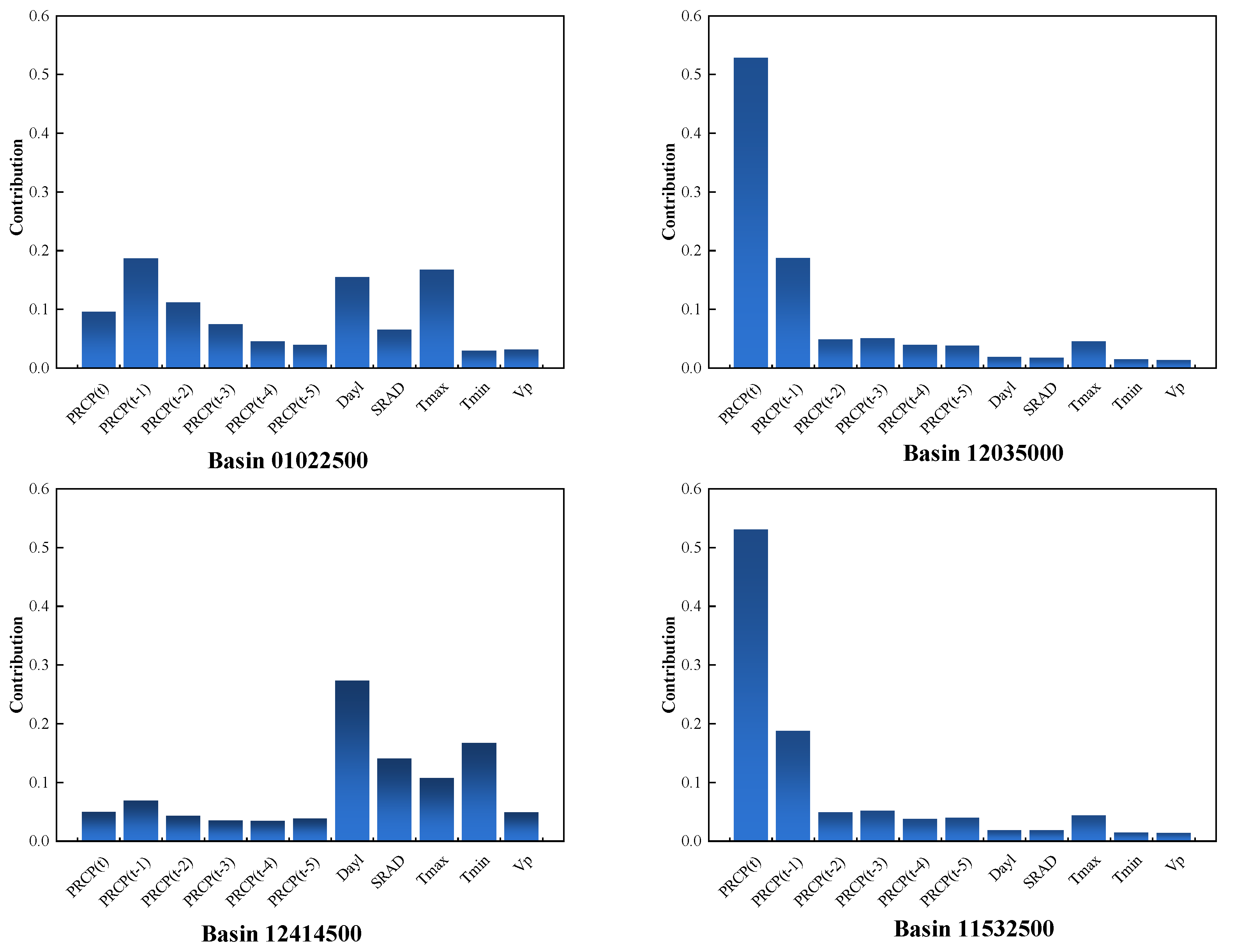
2.1.1. Model Input Selection

Incorporating meteorological and hydrological data into runoff prediction models can enhance their accuracy [43], including variables such as precipitation, temperature, and evaporation [44,45,46,47], with precipitation considered the most important input factor [48]. To mitigate the impact of redundant features on data-driven model prediction accuracy, this study employs Random Forest (RF) for initial feature selection of the model input factors. Random Forest is an ensemble learning algorithm that uses decision trees as base learners and is widely applied in regression prediction and high-dimensional feature selection [42,49]. In this study, the calculation of feature importance in Random Forest utilizes the out-of-bag (OOB) data’s classification accuracy as the evaluation criterion. Assuming there are $A$ decision trees in the Random Forest, the formula for calculating feature importance is as follows.

$$FI=\frac{1}{A}{\displaystyle \sum (e_{OOB2}-e_{OOB1})}$$

(1)

where $FI$ represents the importance of the current data, $e_{OOB1}$ is the error rate obtained by the Random Forest model before variable alteration, and $e_{OOB2}$ is the error rate of the Random Forest model after variable alteration.

2.1.2. Benchmark Model Establishment

Runoff sequences typically consist of both linear and nonlinear components [10]. In fact, there is no universal model that can proficiently capture both linear and nonlinear relationships. In different watersheds, the effectiveness of each model may be different. We have chosen eight commonly used data-driven models in hydrological forecasting, including two statistical models, four machine-learning models, and two deep-learning models [4,6,8,9,11,12,13,14]. We selected three best-performing models as inputs for multi-model ensemble method. Furthermore, each model is represented using abbreviations as shown in

Table 1. Attributes and abbreviations of benchmark models.

Model	Abbreviation	Model Type
Bayesian Ridge Regression	BR	Statistical Model 1
Linear Regression	LR	Statistical Model 2
Gradient Boosting Decision Tree	GBDT	Machine Learning Model 1
Back Propagation Neural Network	BP	Machine Learning Model 2
Random Forest	RF	Machine Learning Model 3
HistGradient Boosting Regressor	HistG	Machine Learning Model 4
Long Short-Term Memory	LSTM	Deep Learning Model 1
Gate Recurrent Unit	GRU	Deep Learning Model 2

.

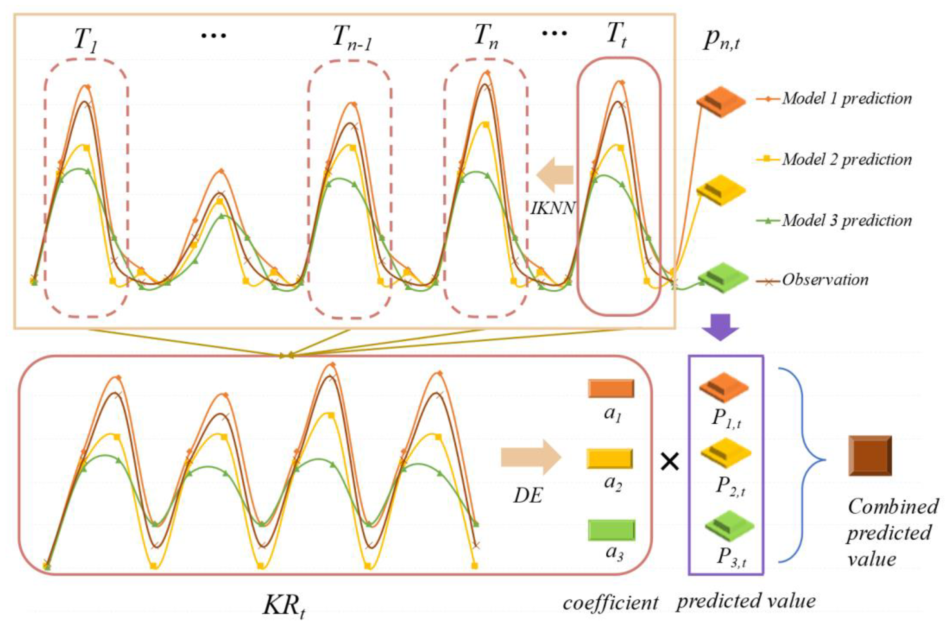
2.2. The Improved K-Nearest Neighbors Method

Traditional K-Nearest Neighbors (KNN) algorithms in runoff forecasting and error correction determine neighboring samples by computing the Euclidean distance between the target sample and other samples [32,34,50,51,52]. For two samples $X_i\left(x_1,\cdots ,x_N\right)$ and $Y_i\left(y_1,\cdots ,y_N\right)$ in an N-dimensional space, the Euclidean distance between $X_i$ and $Y_i$ can be represented as

$$d_{XY}=\sqrt[]{{\displaystyle \sum _{k=1}^N{(x_k-y_k)}^2}}$$

(2)

where $d_{XY}$ is the Euclidean distance between samples; $N$ is the dimensionality of the samples.

The Euclidean distance calculation assumes equal weighting for each dimension, which may not be suitable for runoff sequences characterized by nonlinearity, randomness, and complexity [53]. For instance, a large flow feature’s absolute error can disproportionately affect the similarity ratio of the entire feature vector. In contrast, Pearson Correlation Coefficient (PCC) is not influenced by the magnitude of flow and is suitable for calculating the correlation between flow values of different scales. Introducing PCC into the similarity distance calculation of multi-dimensional runoff sequences can effectively reduce the impact of high-flow characteristic points on similarity selection. The application of PCC in the K-Nearest Neighbor (KNN) algorithm requires adherence to conditions such as linear assumptions, normal distribution assumptions, and equidistant assumptions. Despite the nonlinear and non-normally distributed characteristics of hydrological data, PCC plays a crucial role in the KNN algorithm by capturing the correlation between runoff time series and reducing the influence of flow magnitudes on the results. This aligns with the suitable application scenario for PCC.

This study proposes a novel multidimensional K-Nearest Neighbor (KNN) method. It is based on constructing a distance function for multi-dimensional hydrological sequences using correlation coefficients to enhance the data classification capabilities of the KNN algorithm within multi-dimensional runoff sequences. The specific steps are as follows.

(1) Update the target vector set and historical vector set. Assuming the current prediction time is $t$, the historical vector set $H_t$ consists of $n$ forecast value vectors, denoted as $P_{t,i}\left(p_{1,i},\cdots ,p_{t-2,i},p_{t-1,i}\right)$, and one observed value vector, represented as $O_t\left(o_1,\cdots ,o_{t-2},o_{t-1}\right)$, including historical multi-model forecast values and observed values up to time $t-1$. The target vector set $T_t$ consists of $n$ forecast value vectors with a length of $s$, denoted as $P_{t,n}^{\prime }\left(q_{t-s,i},\cdots ,q_{t-2,i},q_{t-1,i}\right)$, and one observed value vector with a length of $s$, represented as $O_t^{\prime }\left(o_{t-s},\cdots ,o_{t-2},o_{t-1}\right)$. As the observed and forecast data are continuously updated, the vector data in the historical vector set $H_t$ and the target vector set $T_t$ are constantly updated with the latest forecast values and observed values. However, the number of samples in each target vector remains constant at $s$.

$$T_t=\left\{\begin{array}{c}{P}_{t,1}^{\prime }\left(p_{t-s,1},\cdots ,p_{t-2,1},p_{t-1,1}\right)\\ P_{t,2}^{\prime }\left(p_{t-s,2},\cdots ,p_{t-2,2},p_{t-1,2}\right)\\ \cdots \\ \begin{array}{c}{P}_{t,n}^{\prime }\left(p_{t-s,n},\cdots ,p_{t-2,n},p_{t-1,n}\right)\\ O_t^{\prime }\left(o_{t-s},\cdots ,o_{t-2},o_{t-1}\right)\end{array}\end{array}\right\},H_t=\left\{\begin{array}{c}{P}_{t,1}\left(p_{1,1},\cdots ,p_{t-2,1},p_{t-1,1}\right)\\ P_{t,2}\left(p_{1,2},\cdots ,p_{t-2,2},p_{t-1,2}\right)\\ \cdots \\ \begin{array}{c}{P}_{t,n}\left(p_{1,n},\cdots ,p_{t-2,n},p_{t-1,n}\right)\\ O_t\left(o_1,\cdots ,o_{t-2},o_{t-1}\right)\end{array}\end{array}\right\}$$

(3)

where $p_{t,n}$ represents the prediction of the nth model at time $t$, $o_t$ is the observed value at time $t$, and $s$ is the length of the target vector.

(2) Matching Nearest Neighbor Set. When the prediction time is $t$, the historical vector set $H_t$ can extract a set of $t-s$ vectors that are the same size as the target vector set $T_t$. The distance between the collected set and the target vector set is the sum of the correlation between the target vector set B and the corresponding prediction value vector and observed value vector in this set, denoted as $D_{t+ext}(ext=s-t+1,\cdots ,-1,0)$. The formula can be expressed as

$$\begin{array}{l}{P}_{t+ext,n}^{\prime }=\left(p_{t-s+ext,n},\cdots ,p_{t-2+ext,n},p_{t-1+ext,n}\right)\\ O_{t+ext}^{\prime }=\left(o_{t-s+ext},\cdots ,o_{t-2+ext},o_{t-1+ext}\right)\\ D_{t+ext}={\displaystyle \sum _{i=1}^n{r}_{P_{t+ext,i}^{\prime },P_{t,i}^{\prime }}}+r_{O_{t+ext}^{\prime },O_t^{\prime }}\end{array}$$

(4)

where $ext$ represents the time interval, $D_{t+ext}$ is the distance between the target vector set at time $t$ and the extracted vector set from the historical vector set, and $r_{P_{t+ext,i}^{\prime },P_{t,i}^{\prime }}$ is the distance between the target vector set and the i-th model’s predicted value vector in the extracted vector set, while $r_{O_{t+ext}^{\prime },O_t^{\prime }}$ represents the distance between the target vector set and the observed value vector in the extracted vector set.

To identify the most proximate similar target set to the current prediction time, the extracted vector set is sorted in ascending order based on the value of $D_{t+ext}$. The quantification of the correlation is carried out using the Pearson Correlation Coefficient (PCC). For two samples, $X_i\left(x_1,\cdots ,x_N\right)$ and $Y_i\left(y_1,\cdots ,y_N\right)$, in an N-dimensional space, the correlation coefficient between $X_i$ and $Y_i$ can be represented as follows:

$$r_{XY}=\frac{{\displaystyle \sum _{i=1}^N(x_i-\overline{x})}(y_i-\overline{y})}{\sqrt{{\displaystyle \sum _{i=1}^N{(x_i-\overline{x})}^2}{\displaystyle \sum _{i=1}^s{(y_i-\overline{y})}^2}}}$$

(5)

2.3. The Multi-Model Ensemble Method Based on the Improved KNN Algorithm

This section introduces a multi-model ensemble method based on an enhanced K-Nearest Neighbor (KNN) approach to enhance the capabilities of data-driven machine learning models in runoff prediction. As shown in Figure 1, the IKNN-MME method consists of three key steps. Step 1 involves utilizing the enhanced KNN method to extract historically similar samples and introducing the optimally selected similar target set into the weight calibration of the ensemble model. Step 2 involves calculating the weight of each model using the error distribution characteristics of the prediction results and a local error minimization criterion. Step 3 involves dynamically adjusting the model weights at different times and synthesizing the time-varying weights of each model to obtain comprehensive prediction results.

As shown in Figure 2, the specific implementation process and method details are explained below. Initially, multiple heterogeneous data-driven prediction models are selected for runoff forecasting. The forecast results, in conjunction with the observed values, constitute the target vector set and the historical vector set, respectively. Based on the principle of feature space classification using the improved KNN algorithm, we search for $k$ similar vector sets $R_t$ within the historical vector set at the current forecast time. These sets are combined to create a set defined as a similar sample set $K{R}_t$, which includes $n$ forecast value vectors and 1 observed value vector. Each vector contains $k\ast s$ values. The mathematical expression is as follows. In this study, three models were carefully selected as the input for the multi-model ensemble from the eight baseline models. These three sets of streamflow forecast sequences, along with one observed streamflow sequence, were used as model samples, i.e., n = 3.

$$K{R}_t=\left\{\begin{array}{c}{P}_{t+ex{t}_1,1}^{\prime },\cdots ,P_{t+ex{t}_{k-1`},1}^{\prime },P_{t+ex{t}_k,1}^{\prime }\\ \begin{array}{c}{P}_{t+ex{t}_1,2}^{\prime },\cdots ,P_{t+ex{t}_{k-1`},2}^{\prime },P_{t+ex{t}_k,2}^{\prime }\\ \cdots \end{array}\\ P_{t+ex{t}_1,n}^{\prime },\cdots ,P_{t+ex{t}_{k-1`},n}^{\prime },P_{t+ex{t}_k,n}^{\prime }\\ O_{t+ex{t}_1}^{\prime },\cdots ,O_{t+ex{t}_{k-1}}^{\prime },O_{t+ex{t}_k}^{\prime }\end{array}\right\}$$

(6)

where $K{R}_t$ is the target similar sample set, and $ex{t}_k$ represents the time interval between the similar vector set and the target vector set.

Next, based on the principle of similarity, the optimal model combination strategy from the similar sample set is employed as the combination strategy for the multi-model forecast results at the current time. To extract error distribution characteristics from the predictions of multiple models in a similar feature set, a multivariate regression model is constructed, as shown in Equation (7). Based on this, the optimal weights are determined using a minimum error criterion, and the differential evolution algorithm [54] is used for the optimal weighting of the multiple models, with the objective function shown in Equation (8).

$$\left\{\begin{array}{c}{o}_{t+ex{t}_1-s}={\alpha }_1{p}_{t+ex{t}_1-s,1}+\cdots +{\alpha }_{i-1}{p}_{t+ex{t}_1-s,n-1}+{\alpha }_i{p}_{t+ex{t}_1-s,n}\\ \begin{array}{c}\begin{array}{c}\begin{array}{c}\cdots \\ o_{t+ex{t}_1-1}={\alpha }_1{p}_{t+ex{t}_1-1,1}+\cdots +{\alpha }_{i-1}{p}_{t+ex{t}_1-1,n-1}+{\alpha }_i{p}_{t+ex{t}_1-1,n}\end{array}\\ \cdots \end{array}\\ \begin{array}{c}{o}_{t+ex{t}_k-s}={\alpha }_1{p}_{t+ex{t}_k-s,1}+\cdots +{\alpha }_{i-1}{p}_{t+ex{t}_k-s,n-1}+{\alpha }_i{p}_{t+ex{t}_k-s,n}\\ \cdots \end{array}\end{array}\\ o_{t+ex{t}_k-1}={\alpha }_1{p}_{t+ex{t}_k-1,1}+\cdots +{\alpha }_{i-1}{p}_{t+ex{t}_k-1,n-1}+{\alpha }_i{p}_{t+ex{t}_k-1,n}\end{array}\right.$$

(7)

$$\begin{array}{c}\min f(\overrightarrow{\alpha })=\left|{\displaystyle \sum _{j=1}^{s\ast k}({\alpha }_1{p}_{t_j,1}+\cdots {\alpha }_{n-1}{p}_{t_j,n-1}+{\alpha }_n{p}_{t_j,n}}-o_{t_j})/o_{t_j}\right|\\ \overrightarrow{\alpha }=({\alpha }_1,\cdots ,{\alpha }_n)\end{array}$$

(8)

where $a_i$ is the weight of the i-th benchmark model; $p_{n,t_j}$ and $o_{t_j}$ is the forecast value and observed value in the j-th vector at time $t$ within the similar sample set $K{R}_t$.

The data in the target vector set continuously update over time. Different time-varying weights are calculated based on data from different similar sample sets to achieve dynamic updates of model weights. Finally, combining the time-varying weights with the model predictions yields the forecasted values as follows.

$$P_t={\displaystyle \sum _{i=1}^n{a}_i{p}_{t,i}}$$

(9)

2.4. Method Evaluation Metric

In this paper, three evaluation metrics are utilized to assess the performance of different models. The descriptions of these evaluation metrics are as follows.

(1) Nash–Sutcliffe Efficiency Coefficient (NSE)

NSE is the ratio of the sum of squares of the regression to the total sum of squares, reflecting the linear fit between predicted and observed values. The closer the value is to 1, the better the linear fit.

(2) Root Mean Squared Error (RMSE)

RMSE is the square root of the ratio of the square of the deviation between predicted and observed values to the number of observed values, reflecting the degree of dispersion in the dataset.

(3) Mean Absolute Error (MAE)

MAE is the average of the distances between predictions and observations. The mean absolute error can avoid the problem of errors canceling each other out and accurately reflects the size of the actual forecasting error. The specific formulas for these three evaluation metrics are as follows.

$$\mathrm{NSE}=1-\frac{{\displaystyle {\sum }_{i=1}^N{\left(x_i-y_i\right)}^2}}{{\displaystyle {\sum }_{i=1}^N{\left(y_i-{\overline{y}}_i\right)}^2}}$$

(10)

$$\mathrm{MAE}=\frac{1}{N}{\displaystyle \sum _{i=1}^N\left|x_i-y_i\right|}$$

(11)

$$\mathrm{RMSE}=\sqrt{\frac{1}{N}{\displaystyle \sum _{i=1}^N{\left(x_i-y_i\right)}^2}}$$

(12)

where $x$ and $y$ represent the sets of sequences of model prediction values and true values; $x_i$ represents a prediction value; $y_i$ represents an observed value; ${\overline{y}}_i$ is the mean of observed values; and $N$ is the number of prediction and observed values.

3. Case Study

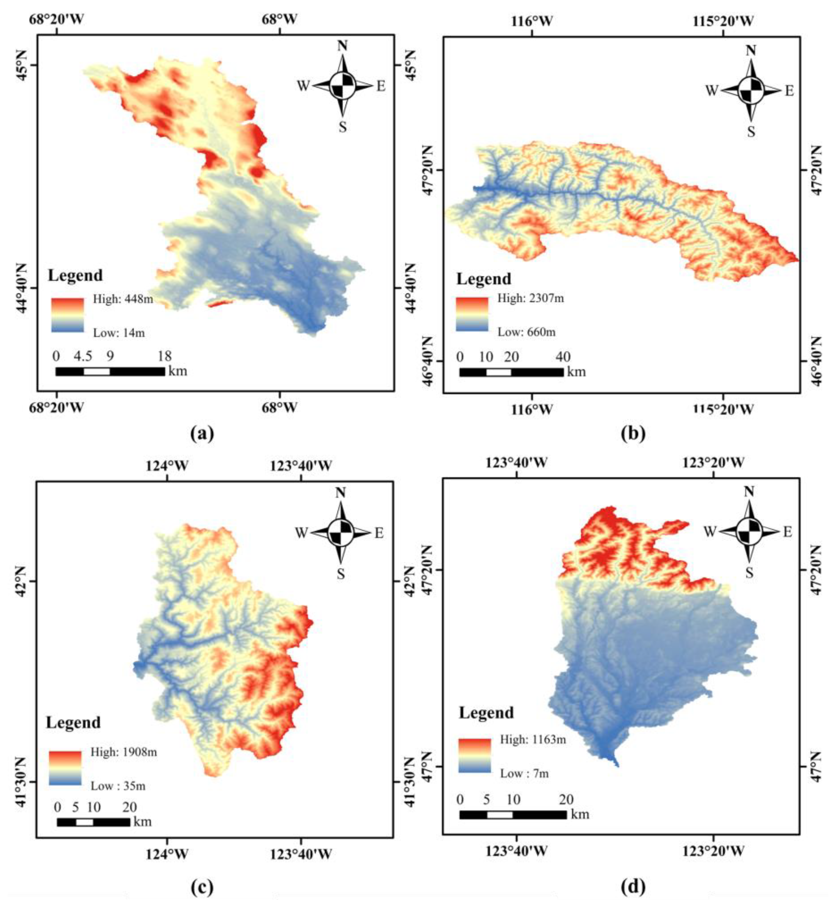
3.1. Study Area and Data

We employed the catchment attributes and meteorology for large-sample studies (CAMELS) dataset [55,56], in which the basins with the least human interference were selected for inclusion in the CAMELS [57,58]. This dataset encompasses average hydro-meteorological time series, catchment attributes, and runoff sequences for 671 catchments within the continental United States. The majority of the hydro-meteorological data in CAMELS falls within the time frame of 1980 to 2014. The meteorological forcing data from CAMELS as model inputs are presented in

Table 2. The forcing variables of four basins.

Variable Name	Description	Units
PRCP	Precipitation	mm/day
SRAD	Solar radiation	W/m2
Tmax	Maximum temperature	°C
Tmin	Minimum temperature	°C
Vp	Vapor pressure	Pa
Dayl	Day length	s

.

To demonstrate the adaptability of the proposed model, four basins with distinct spatial locations and significant variations in hydro-meteorological conditions were chosen as the study areas to assess the runoff simulation performance of the proposed model. These basins include 01022500, 12035000, 12414500, and 11532500 (Figure 3). The former two basins have smaller areas, moderate slopes, and relatively lower elevations, likely corresponding to hilly or plain regions. The latter two basins have larger areas, steeper slopes, and relatively higher elevations, possibly including mountainous or hilly areas. The characteristics of the four selected basins are detailed in

Table 3. The characteristics of four basins.

Basin Code	Size (km2)	Elevation (m)	Slope (m_km−1)
01022500	620.38	92.68	17.79
12414500	2660.37	1381.41	104.38
11532500	1590.16	725.07	112.11
12035000	768.98	149.30	29.35

. The daily hydro-meteorological and runoff data for these watersheds were sequentially divided into training and testing sets, accounting for 80% and 20% of the total data, respectively. The daily streamflow time series was used as model outputs, and the important forcing variables time series were selected as outputs for modeling. The descriptive statistics of the streamflow at the four basins are provided in

Table 4. Descriptive statistics of streamflow data.

Basin Code	01022500	12414500	11532500	12035000
Statistics	Training
MAXIMUM (m3/s)	6790.00	33,900.00	91,200.00	51,800.00
MINIMUM (m3/s)	12.00	105.00	172.00	147.00
MEAN (m3/s)	487.53	2239.04	3640.09	2086.57
Standard Deviation (m3/s)	577.97	2692.87	6247.83	2918.35
Coefficient of Variation	1.19	1.20	1.72	1.40
Statistics	Testing
MAXIMUM (m3/s)	6160.00	22,000.00	76,900.00	34,400.00
MINIMUM (m3/s)	37.00	140.00	190.00	204.00
MEAN (m3/s)	593.45	2428.78	3462.30	2104.60
Standard Deviation (m3/s)	635.49	3222.77	5741.19	2585.62
Coefficient of Variation	1.07	1.33	1.66	1.23

. The training period encompassed 1 January 1980, to 19 October 2007, while the testing period ranged from 20 October 2007 to 30 September 2014. The training set was used for model parameter training, while the testing set was employed to evaluate model performance.

3.2. Data Pre-Processing

(1) Normalized processing

To eliminate the influence of unit and scale differences between features, the feature inputs are normalized using Equation (13). The normalized data fall in the range of [0, 1]:

$$e_{norm}=\frac{e_i-e_{\min }}{e_{\max }-e_{\min }}$$

(13)

where $e_{norm}$ is the normalized values, $e_i$ is the i-th observed values, and $e_{\min }$ and $e_{\max }$ are minimum and maximum values.

(2) Feature selection

Rainfall, as the most significant factor in runoff forecasting, was considered along with the past 5 days’ rainfall and single-day SRAD, Tmax, Tmin, Vp, and Dayl, totaling 11 predictors for input into the Random Forest feature selection model. Feature importance is computed using the out-of-bag (OOB) data error rate as the evaluation metric, and all obtained importance scores are normalized. The results are illustrated in Figure 4, and the top five contributing factors were selected for each of the four basins as the input feature factors for the data-driven model.

4. Results and Discussion

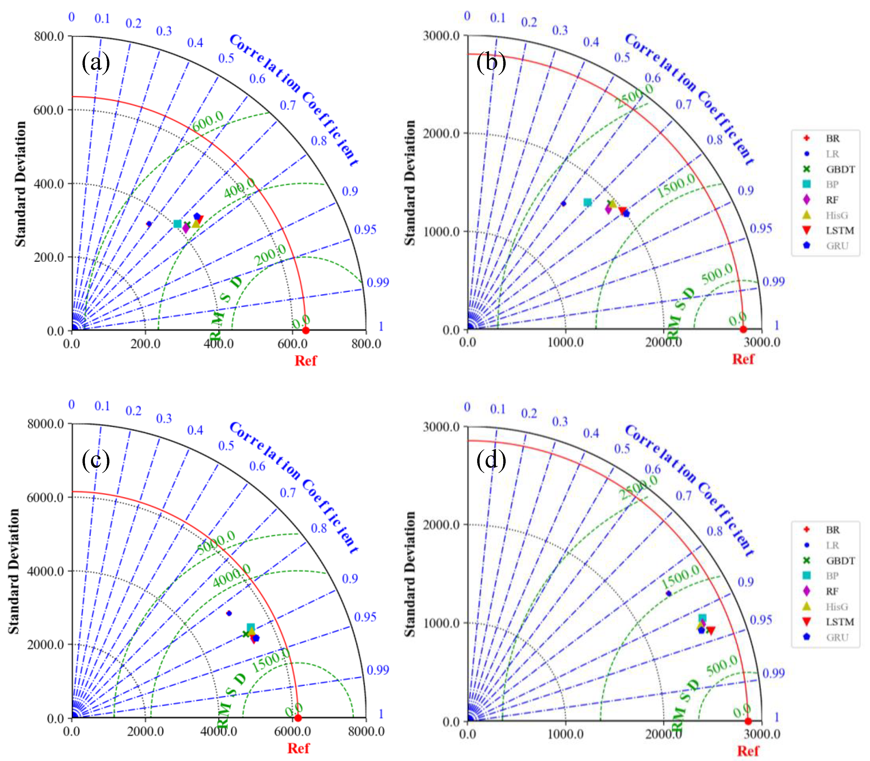
4.1. Runoff Prediction Results of Benchmark Model

In this section, the comprehensive performance of eight data-driven models in runoff forecasting for four basins was compared to determine the three best baseline models for each basin. The hyperparameter adjustment for the benchmark model was refined via iterative experimentation, resulting in a reduction in manual tuning. The quantities of input and output nodes were set at 5 and 1, respectively. To ensure the comprehensive training of the deep-learning model, the value of the epochs was configured to 100. The runoff forecasting results are presented in

Table 5. Predictive performance of 8 baseline models for the 4 basins.

Area	Model	NSE	RMSE (m3/s)	MAE (m3/s)
01025000	BR	0.32	523.1	323.0
	LR	0.32	523.1	323.0
	GBDT	0.52	441.6	258.0
	BP	0.47	464.8	272.7
	RF	0.52	439.9	253.3
	HistG	0.55	425.8	245.5
	LSTM	0.55	426.3	248.0
	GRU	0.54	431.3	255.8
	average	0.47	459.5	272.4
12414500	BR	0.38	2530.0	1576.8
	LR	0.38	2529.9	1577.1
	GBDT	0.53	2221.5	1228.7
	BP	0.50	2274.9	1288.0
	RF	0.55	2162.8	1170.7
	HistG	0.57	2122.2	1161.1
	LSTM	0.58	2095.4	1127.4
	GRU	0.58	2094.3	1120.9
	average	0.51	2253.9	1281.4
11532500	BR	0.67	3297.7	1866.4
	LR	0.67	3297.8	1866.7
	GBDT	0.78	2687.8	1536.7
	BP	0.78	2689.3	1561.4
	RF	0.79	2637.0	1535.1
	HistG	0.78	2718.7	1543.3
	LSTM	0.80	2557.7	1524.3
	GRU	0.79	2626.9	1534.6
	average	0.76	2814.1	1621.1
12035000	BR	0.70	1425.9	928.8
	LR	0.70	1425.9	928.9
	GBDT	0.83	1069.4	669.7
	BP	0.82	1096.3	723.2
	RF	0.82	1098.5	674.4
	HistG	0.82	1099.9	670.8
	LSTM	0.84	1034.5	653.8
	GRU	0.84	1047.2	658.7
	average	0.79	1162.2	738.5

. For Basin 01025000, the models HistG, LSTM, and GRU exhibited superior to the other models. Basin 12414500 shows similar forecasting capabilities to Basin 01025000, with HistG, LSTM, and GRU outperforming the other models. In the case of Basins 11532500 and 12035000, the selected three baseline models were RF, LSTM, and GRU, and GBDT, LSTM, and GRU, respectively. Overall, deep-learning models demonstrated higher predictive accuracy compared to machine-learning models, while machine-learning models outperformed statistical models. Additionally, it can be observed from Table 5 that the forecasting performance for Basins 12035000 and 11,532,500 is significantly better than that for Basins 01025000 and 12414500. The average NSE for Basin 12035000 improved by 67.81% and 56.39% compared to Basins 01025000 and 12414500, respectively. For Basin 11532500, the average NSE improved by 59.96% and 49.08% compared to Basins 01025000 and 12414500, respectively. This indicates that the contribution of feature factors effectively impacts the predictive performance of data-driven models. When the input feature factors have a greater contribution to the output features, meaning a stronger correlation, the model’s predictive capabilities also improve accordingly. Additionally, Taylor diagrams, as shown in Figure 5, were generated to visually summarize the prediction performance of the eight different data-driven methods. Observation points are marked in red, and the closer the model prediction points are to the observation marks, the better the model prediction performance.

In a previous study [6], the authors similarly employed linear models, machine-learning models, and deep-learning models (AR, ANN, and LSTM) to carry out runoff predictions for 671 watersheds in the CAMELS dataset under different data integration and comparative scenarios. The obtained median NSE values are 0.554, 0.650, and 0.714, respectively. The research indicated that LSTM exhibited significant advantages compared to the traditional statistical methods (AR). In the present study, baseline models were constructed, yielding results similar to LSTM, suggesting that the baseline models developed in this study can serve as effective tools for runoff prediction in the study area.

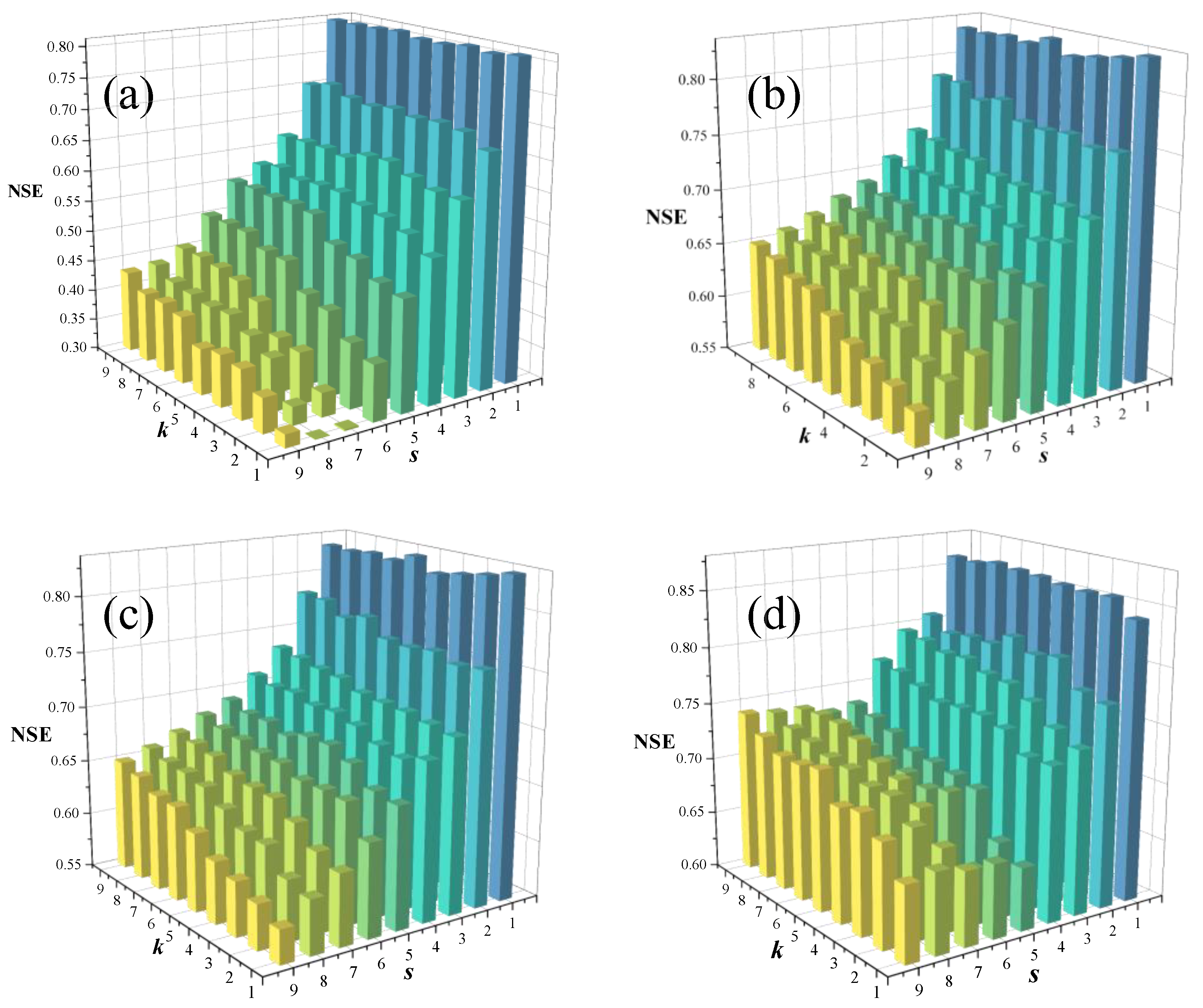
4.2. Parameters Preferences

The IKNN-MME algorithm proposed in this study relies on two critical parameters: $k$ and $s$. A grid search method is employed to optimize these parameters, with the Nash–Sutcliffe efficiency (NSE) used as the evaluation metric for selecting the model that performs best. For each basin, the top three models with the most promising predictive performance from the eight available data-driven models are chosen as input for the IKNN-MME. Subsequently, a grid search is conducted to assess the performance of the IKNN-MME model for various $k$ values with $s$ ranging from 1 to 9. The results, as illustrated in Figure 6, consistently indicate that the IKNN-MME model performs optimally when $s$ is set to 1, where it exclusively incorporates the data features from the nearest neighbor within a single unit as its target feature set. However, with increasing values of $s$, the model’s accuracy substantially diminishes. This suggests that an excessive number of data features might adversely affect the precision of the model combination. Remarkably, when $s$ is set to 1, the performance of the IKNN-MME model remains relatively consistent across different $k$ values, allowing for a constant $k$ value of 5 for subsequent calculations.

The parameter $k$ is crucial in the KNN algorithm, and in the application of other KNN algorithms in the runoff prediction [34,40], the model’s prediction accuracy rapidly improves as $k$ increases from 1. However, as $k$ continues to rise to its optimal value, the model’s prediction accuracy exhibits a slow decline. In this study, the sensitivity of the parameter $k$ is not pronounced. When $k$ is varied at $s$ = 1, the model’s prediction accuracy does not show a clear trend of improvement followed by deterioration. This is because the KNN algorithm in this study is not directly applied to the model results but is used to determine the combination weights of multiple models. As the number of samples with different similarity levels increases, the corrective effect on the model weights gradually decreases, resulting in no significant changes in the model results with the increase in $k$. When $s$ increases, an increase in $k$ actually leads to a reduction in the model’s prediction accuracy. This is attributed to the larger $k$ values accompanying a continuous decrease in the threshold for determining similarity. Dissimilar sample points persistently interfere with the model results, thereby reducing accuracy.

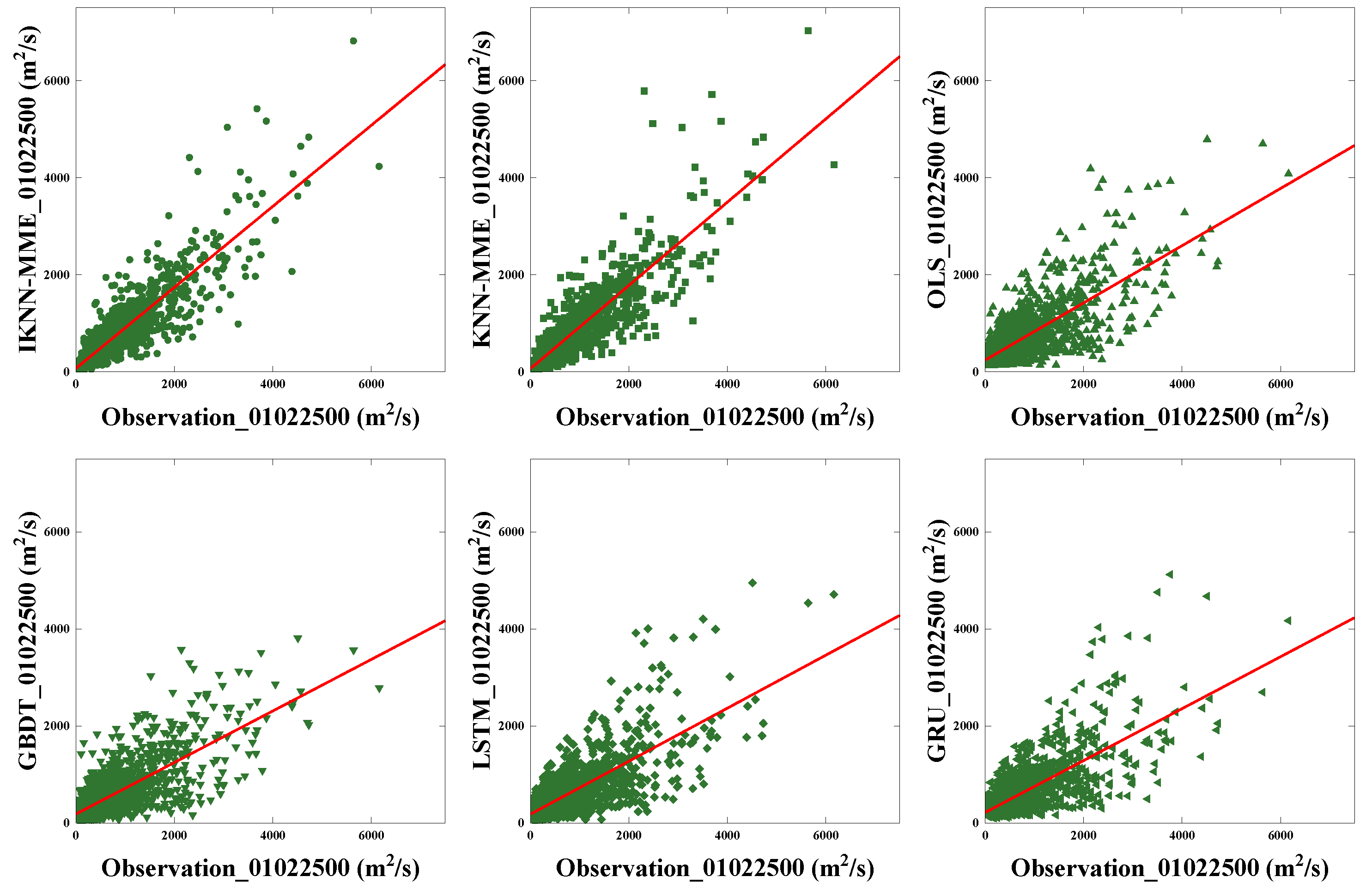
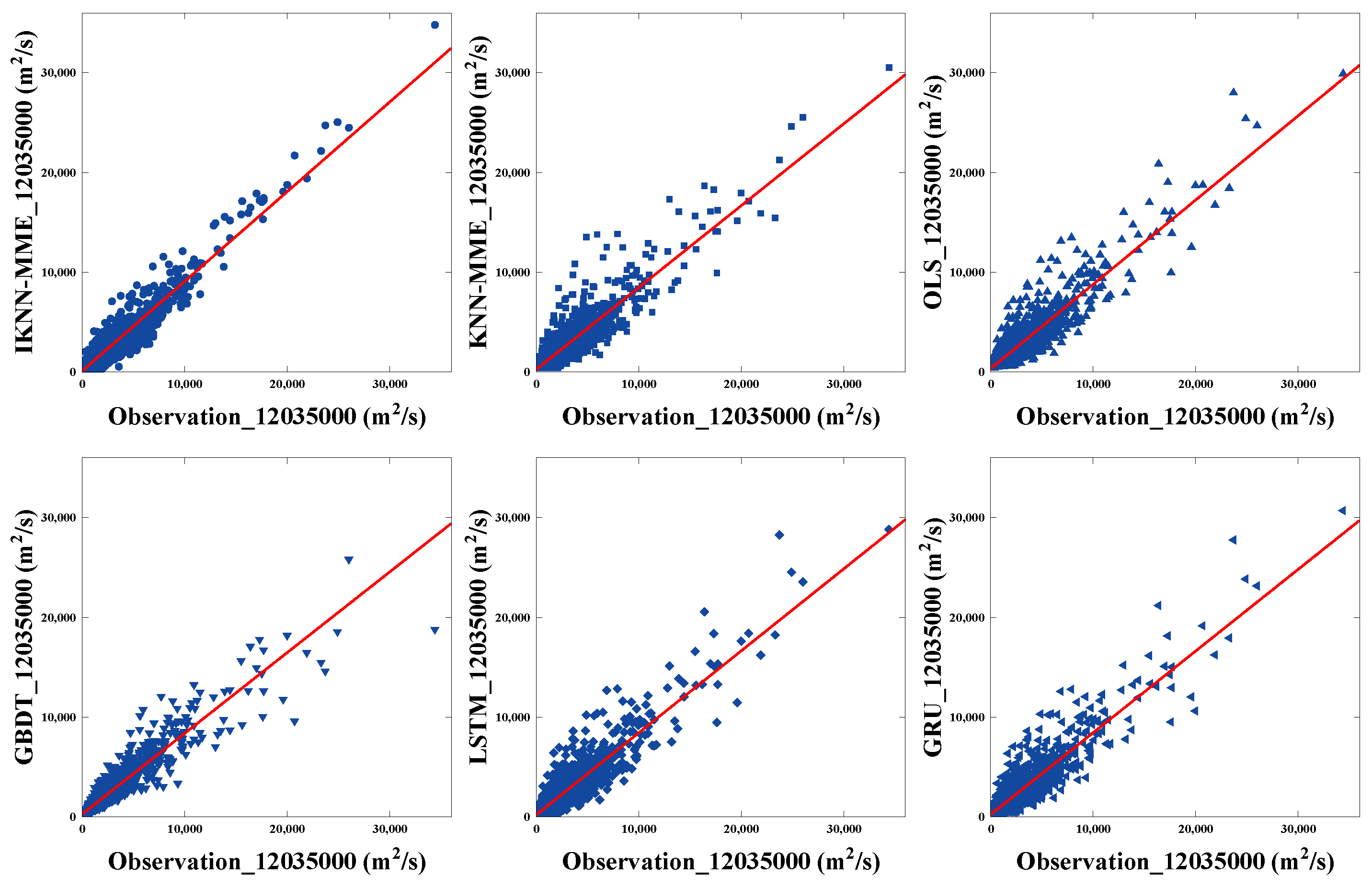
4.3. Comparisons of Multi-Model Ensemble Forecasting Methods

In this section, three different multi-model ensemble forecasting methods were applied to the three best-performing benchmark models in each of the four basins. These methods include IKNN-MME, a multi-model ensemble method based on traditional KNN (KNN-MME), and ordinary least squares (OLS), the KNN-MME method uses the Euclidean distance in the comparison of similar sample sets.

Table 6. Performance comparison of different ensemble models and benchmark models.

Basin Code	Model	NSE	RMSE (m3/s)	MAE (m3/s)
01022500	IKNN-MME	0.81	274.7	137.4
	KNN-MME	0.80	281.2	138.7
	OLS	0.56	419.7	262.9
	HistG	0.55	425.8	245.5
	LSTM	0.55	426.3	248.0
	GRU	0.54	431.3	255.8
12414500	IKNN-MME	0.84	1290.2	553.6
	KNN-MME	0.83	1337.3	561.6
	OLS	0.56	2149.0	1262.7
	HistG	0.57	2122.2	1161.1
	LSTM	0.58	2095.4	1127.4
	GRU	0.58	2094.3	1120.9
11532500	IKNN-MME	0.89	1939.3	808.3
	KNN-MME	0.88	2030.1	822.3
	OLS	0.80	2583.3	1505.2
	RF	0.79	2637.0	1535.1
	LSTM	0.80	2557.7	1524.3
	GRU	0.79	2626.9	1534.6
12035000	IKNN-MME	0.89	875.8	372.0
	KNN-MME	0.87	925.2	382.5
	OLS	0.84	1047.9	669.4
	GBDT	0.83	1069.4	669.7
	LSTM	0.84	1034.5	653.8
	GRU	0.84	1047.2	658.7

displays the corresponding statistical data for the six models in each of the basins. As seen in Table 6, for Basin 01025000, all three multi-model ensemble methods are capable of enhancing forecasting abilities to some extent. IKNN-MME, KNN-MME, and OLS improve the NSE by 47.57%, 45.94%, and 2.38%, respectively, compared to the best-performing benchmark model HistG. For Basin 12414500, IKNN-MME and KNN-MME increase the NSE by 45.44% and 43.37%, respectively, while OLS reduces it by 3.90%, relative to the best benchmark model GRU. In the case of Basin 11532500, IKNN-MME and KNN-MME result in NSE improvements of 10.55% and 9.18%, respectively, compared to the best benchmark model LSTM, whereas OLS decreases the NSE by 0.55%. In Basin 12035000, IKNN-MME and KNN-MME enhance the NSE by 5.38% and 3.83%, respectively, compared to the best benchmark model LSTM, while OLS decreases the NSE by 0.46%, multi-model ensemble methods do not always improve single-model accuracy. In the experiments conducted for the four basins, both of the proposed multi-model ensemble forecasting methods, IKNN-MME and KNN-MME, significantly enhance the predictive capabilities of the benchmark models, demonstrating higher accuracy compared to the traditional multi-model ensemble model OLS.

In order to perform a detailed comparison of the developed ensemble model and the baseline models, scatter plots of the test phase results for all investigated sites (i.e., Basins 01022500, 12414500, 11532500, and 12035000) are separately presented in Figure 7, Figure 8, Figure 9 and Figure 10. Figure 7 illustrates the scatter plot generated for Basin 01022500. Clearly, the fitting lines of both the proposed IKNN-MME and KNN-MME methods are closer to the 45-degree line, Compared to the KNN-MME method, the IKNN-MME method demonstrates better accuracy in predicting high flow. Figure 8 displays the scatter plot generated for Basin 12414500. The IKNN-MME method proposed in this study exhibits the best-fitting performance between the observed and predicted values. However, both the IKNN-MME and KNN-MME methods tend to overestimate flow rates, with KNN-MME showing a more severe overestimation, particularly for high flow. Figure 9 and Figure 10 depict the scatter plots for Basins 11532500 and 12035000, respectively. It is evident that the modeling results for Basins 11532500 and 12035000 slightly differ from the other two Basins (01022500 and 12414500). Both the proposed ensemble forecasting model and the baseline models yield good results, with minimal differences. In particular, the forecasting performance of the proposed IKNN-MME and KNN-MME methods is very close, slightly outperforming the baseline models and the OLS method. Overall, for the four basins, the ensemble forecasting sequences calculated by the proposed multi-model integration method show an improved fit with the observed flow sequences compared to the baseline models and the OLS method.

The proposed IKNN-MME method exhibits superior predictive performance across four sites with distinct characteristic attributes compared to both the baseline model and the OLS model. This is a beneficial outcome, considering that the accuracy improvement of ensemble methods over single models requires specific conditions to be met [59]. As indicated in Table 6, the baseline model’s prediction accuracy for Basin 12035000 consistently surpasses that of Basin 11532500. However, the IKNN-MME method for Basin 11532500 achieves better combined prediction accuracy, leading to instances where the OLS model’s prediction accuracy does not consistently outperform that of a single model. It is noteworthy that in peak flow simulations, the IKNN-MME model, compared to the KNN-MME model, yields results closer to the observational values. This suggests that the improved KNN approach effectively mitigates the influence of high-flow characteristic points on the weights of multiple models in runoff sequences, making the predictions more closely aligned with actual values.

The effective role of the IKNN-MME method, based on the enhanced KNN approach, within the existing machine-learning forecasting framework lies in its consideration of the similarity of the historical runoff prediction results to enhance the current predictive performance rather than solely focusing on input factor selection or parameter optimization. Additionally, the model has simple inputs, making it suitable for enhancing the accuracy of most data-driven runoff forecasts and applicable for improving water resource management decisions. Furthermore, compared to the traditional dynamic weighting models, the IKNN-MME model, by using optimized data through an improved KNN, inevitably reduces computational efficiency. However, the parameter optimization results indicate that a smaller K value suffices for satisfactory simulation results, reducing the computational workload for each time step solved by the optimization model and thus lowering the model’s computational demands.

5. Conclusions

To enhance the performance of data-driven models in runoff prediction, this study introduces the Improved K-Nearest Neighbor-based Multi-Model Ensemble method (IKNN-MME). This method, by coupling the improved KNN approach and multi-model ensemble techniques, strengthens the runoff modeling capabilities from both feature data selection and dynamic weighting of multiple models. To validate the model’s practicality, it is applied to runoff prediction in four watersheds in the United States. The results indicate that the performance of individual data-driven models in the study area is limited, especially in watersheds where there is a weak correlation between input factors and runoff. Upon applying the IKNN-MME model for multi-model combination, the model’s predictive Nash–Sutcliffe efficiency (NSE) values are improved from around 0.55 to above 0.80. For peak flow, the IKNN-MME model, based on the improved KNN, exhibits combined results closer to observational values compared to the KNN-MME model based on traditional KNN. This underscores the superiority of the improved IKNN over traditional KNN in multi-model integration, providing a novel approach for enhancing the accuracy of data-driven prediction models. Additionally, this study reveals the following:

(1) Data-driven models exhibit stronger predictive performance when there is a higher correlation between input and output features.

(2) The runoff prediction capabilities of deep-learning models are, to some extent, superior to machine-learning and linear models.

(3) Multi-model ensemble prediction models do not consistently demonstrate a characteristic of consistently improving the baseline model’s prediction ability.

However, the proposed method still has limitations. The IKNN-MME model has a limited capability to enhance the prediction performance of baseline models with already high accuracy, and the computational efficiency of the model is relatively low. Future research directions include improving the computational efficiency of ensemble models, enhancing the accuracy and robustness of the model, obtaining higher-precision runoff prediction results, and ultimately improving water resource management decisions.

References

1. Qiu, H.; Chen, L.; Zhou, J.; He, Z.; Zhang, H. Risk Analysis of Water Supply-Hydropower Generation-Environment Nexus in the Cascade Reservoir Operation. J. Clean. Prod. 2021, 283, 124239. [Google Scholar] [CrossRef]
2. Yi, B.; Chen, L.; Zhang, H.; Singh, V.P.; Jiang, P.; Liu, Y.; Guo, H.; Qiu, H. A Time-Varying Distributed Unit Hydrograph Method Considering Soil Moisture. Hydrol. Earth Syst. Sci. 2022, 26, 5269–5289. [Google Scholar] [CrossRef]
3. Guo, Z.; Moosavi, V.; Leitão, J.P. Data-Driven Rapid Flood Prediction Mapping with Catchment Generalizability. J. Hydrol. 2022, 609, 127726. [Google Scholar] [CrossRef]
4. Liu, G.; Tang, Z.; Qin, H.; Liu, S.; Shen, Q.; Qu, Y.; Zhou, J. Short-Term Runoff Prediction Using Deep Learning Multi-Dimensional Ensemble Method. J. Hydrol. 2022, 609, 127762. [Google Scholar] [CrossRef]
5. Pour, S.H.; Shahid, S.; Sammen, S.S. Chapter 25—Runoff Modeling Using Group Method of Data Handling and Gene Expression Programming. In Handbook of Hydroinformatics; Eslamian, S., Eslamian, F., Eds.; Elsevier: Amsterdam, The Netherlands, 2023; pp. 353–377. ISBN 978-0-12-821962-1. [Google Scholar]
6. Feng, D.; Fang, K.; Shen, C. Enhancing Streamflow Forecast and Extracting Insights Using Long-Short Term Memory Networks with Data Integration at Continental Scales. Water Resour. Res. 2020, 56, e2019WR026793. [Google Scholar] [CrossRef]
7. Naganna, S.R.; Marulasiddappa, S.B.; Balreddy, M.S.; Yaseen, Z.M. Daily Scale Streamflow Forecasting in Multiple Stream Orders of Cauvery River, India: Application of Advanced Ensemble and Deep Learning Models. J. Hydrol. 2023, 626, 130320. [Google Scholar] [CrossRef]
8. Lima, C.H.R.; Lall, U. Climate Informed Monthly Streamflow Forecasts for the Brazilian Hydropower Network Using a Periodic Ridge Regression Model. J. Hydrol. 2010, 380, 438–449. [Google Scholar] [CrossRef]
9. Si, W.; Gupta, H.V.; Bao, W.; Jiang, P.; Wang, W. Improved Dynamic System Response Curve Method for Real-Time Flood Forecast Updating. Water Resour. Res. 2019, 55, 7493–7519. [Google Scholar] [CrossRef]
10. Yang, T.; Zhang, L.; Kim, T.; Hong, Y.; Zhang, D.; Peng, Q. A Large-Scale Comparison of Artificial Intelligence and Data Mining (AI&DM) Techniques in Simulating Reservoir Releases over the Upper Colorado Region. J. Hydrol. 2021, 602, 126723. [Google Scholar] [CrossRef]
11. Nayak, P.C.; Sudheer, K.P.; Rangan, D.M.; Ramasastri, K.S. Short-Term Flood Forecasting with a Neurofuzzy Model. Water Resour. Res. 2005, 41, W04004. [Google Scholar] [CrossRef]
12. Mosavi, A.; Ozturk, P.; Chau, K. Flood Prediction Using Machine Learning Models: Literature Review. Water 2018, 10, 1536. [Google Scholar] [CrossRef]
13. Liang, W.; Luo, S.; Zhao, G.; Wu, H. Predicting Hard Rock Pillar Stability Using GBDT, XGBoost, and LightGBM Algorithms. Mathematics 2020, 8, 765. [Google Scholar] [CrossRef]
14. Kratzert, F.; Klotz, D.; Brenner, C.; Schulz, K.; Herrnegger, M. Rainfall–Runoff Modelling Using Long Short-Term Memory (LSTM) Networks. Hydrol. Earth Syst. Sci. 2018, 22, 6005–6022. [Google Scholar] [CrossRef]
15. Shamseldin, A.Y.; O’Connor, K.M.; Liang, G.C. Methods for Combining the Outputs of Different Rainfall–Runoff Models. J. Hydrol. 1997, 197, 203–229. [Google Scholar] [CrossRef]
16. Chen, L.; Zhang, Y.; Zhou, J.; Singh, V.; Guo, S.; Zhang, J. Real-Time Error Correction Method Combined with Combination Flood Forecasting Technique for Improving the Accuracy of Flood Forecasting. J. Hydrol. 2014, 521, 157–169. [Google Scholar] [CrossRef]
17. Wu, J.; Zhou, J.; Chen, L.; Ye, L. Coupling Forecast Methods of Multiple Rainfall–Runoff Models for Improving the Precision of Hydrological Forecasting. Water Resour. Manag. 2015, 29, 5091–5108. [Google Scholar] [CrossRef]
18. Chevuturi, A.; Tanguy, M.; Facer-Childs, K.; Martínez-de la Torre, A.; Sarkar, S.; Thober, S.; Samaniego, L.; Rakovec, O.; Kelbling, M.; Sutanudjaja, E.H.; et al. Improving Global Hydrological Simulations through Bias-Correction and Multi-Model Blending. J. Hydrol. 2023, 621, 129607. [Google Scholar] [CrossRef]
19. Shin, S.; Her, Y.; Muñoz-Carpena, R.; Khare, Y.P. Multi-Parameter Approaches for Improved Ensemble Prediction Accuracy in Hydrology and Water Quality Modeling. J. Hydrol. 2023, 622, 129458. [Google Scholar] [CrossRef]
20. Xu, C.; Zhong, P.; Zhu, F.; Yang, L.; Wang, S.; Wang, Y. Real-Time Error Correction for Flood Forecasting Based on Machine Learning Ensemble Method and Its Uncertainty Assessment. Stoch. Environ. Res. Risk Assess. 2023, 37, 1557–1577. [Google Scholar] [CrossRef]
21. Wanders, N.; Wood, E.F. Improved Sub-Seasonal Meteorological Forecast Skill Using Weighted Multi-Model Ensemble Simulations. Environ. Res. Lett. 2016, 11, 094007. [Google Scholar] [CrossRef]
22. Liu, G.; Wang, Y.; Qin, H.; Shen, K.; Liu, S.; Shen, Q.; Qu, Y.; Zhou, J. Probabilistic Spatiotemporal Forecasting of Wind Speed Based on Multi-Network Deep Ensembles Method. Renew. Energy 2023, 209, 231–247. [Google Scholar] [CrossRef]
23. Wang, Q.J.; Schepen, A.; Robertson, D.E. Merging Seasonal Rainfall Forecasts from Multiple Statistical Models through Bayesian Model Averaging. J. Clim. 2012, 25, 5524–5537. [Google Scholar] [CrossRef]
24. Zhang, L.; Yang, X. Applying a Multi-Model Ensemble Method for Long-Term Runoff Prediction under Climate Change Scenarios for the Yellow River Basin, China. Water 2018, 10, 301. [Google Scholar] [CrossRef]
25. Raftery, A.E.; Gneiting, T.; Balabdaoui, F.; Polakowski, M. Using Bayesian Model Averaging to Calibrate Forecast Ensembles. Mon. Weather Rev. 2005, 133, 1155–1174. [Google Scholar] [CrossRef]
26. Wang, J.; Bao, W.; Xiao, Z.; Si, W. Multi-Model Integrated Error Correction for Streamflow Simulation Based on Bayesian Model Averaging and Dynamic System Response Curve. J. Hydrol. 2022, 607, 127518. [Google Scholar] [CrossRef]
27. Farfán, J.F.; Cea, L. Improving the Predictive Skills of Hydrological Models Using a Combinatorial Optimization Algorithm and Artificial Neural Networks. Model. Earth Syst. Environ. 2023, 9, 1103–1118. [Google Scholar] [CrossRef]
28. Hajirahimi, Z.; Khashei, M. Weighting Approaches in Data Mining and Knowledge Discovery: A Review. Neural Process Lett. 2023, 55, 1–46. [Google Scholar] [CrossRef]
29. de Amorim, R.C. A Survey on Feature Weighting Based K-Means Algorithms. J. Classif. 2016, 33, 210–242. [Google Scholar] [CrossRef]
30. Akbari, M.; van Overloop, P.J.; Afshar, A. Clustered K Nearest Neighbor Algorithm for Daily Inflow Forecasting. Water Resour. Manag. 2011, 25, 1341–1357. [Google Scholar] [CrossRef]
31. Ran, J.; Cui, Y.; Xiang, K.; Song, Y. Improved Runoff Forecasting Based on Time-Varying Model Averaging Method and Deep Learning. PLoS ONE 2022, 17, e0274004. [Google Scholar] [CrossRef]
32. Liu, K.; Li, Z.; Yao, C.; Chen, J.; Zhang, K.; Saifullah, M. Coupling the K-Nearest Neighbor Procedure with the Kalman Filter for Real-Time Updating of the Hydraulic Model in Flood Forecasting. Int. J. Sediment Res. 2016, 31, 149–158. [Google Scholar] [CrossRef]
33. Delima, A.J.P. An Enhanced K-Nearest Neighbor Predictive Model through Metaheuristic Optimization. Int. J. Eng. Technol. Innov. 2020, 10, 280–292. [Google Scholar] [CrossRef]
34. Yang, M.; Wang, H.; Jiang, Y.; Lu, X.; Xu, Z.; Sun, G. GECA Proposed Ensemble–KNN Method for Improved Monthly Runoff Forecasting. Water Resour. Manag. 2020, 34, 849–863. [Google Scholar] [CrossRef]
35. Ukey, N.; Yang, Z.; Li, B.; Zhang, G.; Hu, Y.; Zhang, W. Survey on Exact kNN Queries over High-Dimensional Data Space. Sensors 2023, 23, 629. [Google Scholar] [CrossRef] [PubMed]
36. Akbari, M.; Afshar, A. Similarity-Based Error Prediction Approach for Real-Time Inflow Forecasting. Hydrol. Res. 2013, 45, 589–602. [Google Scholar] [CrossRef]
37. Modaresi, F.; Araghinejad, S. A Comparative Assessment of Support Vector Machines, Probabilistic Neural Networks, and K-Nearest Neighbor Algorithms for Water Quality Classification. Water Resour. Manag. 2014, 28, 4095–4111. [Google Scholar] [CrossRef]
38. Karlsson, M.; Yakowitz, S. Nearest-Neighbor Methods for Nonparametric Rainfall-Runoff Forecasting. Water Resour. Res. 1987, 23, 1300–1308. [Google Scholar] [CrossRef]
39. Wan, H.; Xia, J.; Zhang, L.; She, D.; Xiao, Y.; Zou, L. Sensitivity and Interaction Analysis Based on Sobol’ Method and Its Application in a Distributed Flood Forecasting Model. Water 2015, 7, 2924–2951. [Google Scholar] [CrossRef]
40. Gauhar, N.; Das, S.; Moury, K.S. Prediction of Flood in Bangladesh Using K-Nearest Neighbors Algorithm. In Proceedings of the 2021 2nd International Conference on Robotics, Electrical and Signal Processing Techniques (ICREST), Dhaka, Bangladesh, 5–7 January 2021; pp. 357–361. [Google Scholar]
41. Liu, D.; Wang, C.; Ji, Y.; Fu, Q.; Li, M.; Ali, S.; Li, T.; Cui, S. Measurement and Analysis of Regional Flood Disaster Resilience Based on a Support Vector Regression Model Refined by the Selfish Herd Optimizer with Elite Opposition-Based Learning. J. Environ. Manag. 2021, 300, 113764. [Google Scholar] [CrossRef]
42. Yang, B.; Chen, L.; Singh, V.P.; Yi, B.; Leng, Z.; Zheng, J.; Song, Q. A Method for Monthly Extreme Precipitation Forecasting with Physical Explanations. Water 2023, 15, 1545. [Google Scholar] [CrossRef]
43. Puttinaovarat, S.; Horkaew, P. Flood Forecasting System Based on Integrated Big and Crowdsource Data by Using Machine Learning Techniques. IEEE Access 2020, 8, 5885–5905. [Google Scholar] [CrossRef]
44. Ahmad, M.; Al Mehedi, M.A.; Yazdan, M.M.S.; Kumar, R. Development of Machine Learning Flood Model Using Artificial Neural Network (ANN) at Var River. Liquids 2022, 2, 147–160. [Google Scholar] [CrossRef]
45. Wang, S.; Sun, M.; Wang, G.; Yao, X.; Wang, M.; Li, J.; Duan, H.; Xie, Z.; Fan, R.; Yang, Y. Simulation and Reconstruction of Runoff in the High-Cold Mountains Area Based on Multiple Machine Learning Models. Water 2023, 15, 3222. [Google Scholar] [CrossRef]
46. Yi, B.; Chen, L.; Yang, B.; Li, S.; Leng, Z. Influences of the Runoff Partition Method on the Flexible Hybrid Runoff Generation Model for Flood Prediction. Water 2023, 15, 2738. [Google Scholar] [CrossRef]
47. Yi, B.; Chen, L.; Liu, Y.; Guo, H.; Leng, Z.; Gan, X.; Xie, T.; Mei, Z. Hydrological Modelling with an Improved Flexible Hybrid Runoff Generation Strategy. J. Hydrol. 2023, 620, 129457. [Google Scholar] [CrossRef]
48. Chen, X.; Zhang, L.; Gippel, C.J.; Shan, L.; Chen, S.; Yang, W. Uncertainty of Flood Forecasting Based on Radar Rainfall Data Assimilation. Adv. Meteorol. 2016, 2016, e2710457. [Google Scholar] [CrossRef]
49. Qiao, X.; Peng, T.; Sun, N.; Zhang, C.; Liu, Q.; Zhang, Y.; Wang, Y.; Shahzad Nazir, M. Metaheuristic Evolutionary Deep Learning Model Based on Temporal Convolutional Network, Improved Aquila Optimizer and Random Forest for Rainfall-Runoff Simulation and Multi-Step Runoff Prediction. Expert Syst. Appl. 2023, 229, 120616. [Google Scholar] [CrossRef]
50. Shamseldin, A.Y.; O’Connor, K.M. A Nearest Neighbour Linear Perturbation Model for River Flow Forecasting. J. Hydrol. 1996, 179, 353–375. [Google Scholar] [CrossRef]
51. Liu, Z.; Guo, S.; Zhang, H.; Liu, D.; Yang, G. Comparative Study of Three Updating Procedures for Real-Time Flood Forecasting. Water Resour. Manag. 2016, 30, 2111–2126. [Google Scholar] [CrossRef]
52. Ebrahimi, E.; Shourian, M. River Flow Prediction Using Dynamic Method for Selecting and Prioritizing K-Nearest Neighbors Based on Data Features. J. Hydrol. Eng. 2020, 25, 04020010. [Google Scholar] [CrossRef]
53. Wang, W.-C.; Chau, K.-W.; Cheng, C.-T.; Qiu, L. A Comparison of Performance of Several Artificial Intelligence Methods for Forecasting Monthly Discharge Time Series. J. Hydrol. 2009, 374, 294–306. [Google Scholar] [CrossRef]
54. Storn, R. Differential Evolution—A Simple and Efficient Heuristic for Global Optimization over Continuous Spaces. J. Glob. Optim. 1997, 11, 341–359. [Google Scholar] [CrossRef]
55. Addor, A.N.; Mizukami, M.; Clark, M.P. Catchment Attributes for Large-Sample Studies; UCAR/NCAR: Boulder, CO, USA, 2017. [Google Scholar] [CrossRef]
56. Newman, A.; Sampson, K.; Clark, M.P.; Bock, A.; Viger, R.J.; Blodgett, D. A Large-Sample Watershed-Scale Hydrometeorological Dataset for the Contiguous; UCAR/NCAR: Boulder, CO, USA, 2014. [Google Scholar] [CrossRef]
57. Newman, A.J.; Clark, M.P.; Sampson, K.; Wood, A.; Hay, L.E.; Bock, A.; Viger, R.J.; Blodgett, D.; Brekke, L.; Arnold, J.R.; et al. Development of a Large-Sample Watershed-Scale Hydrometeorological Data Set for the Contiguous USA: Data Set Characteristics and Assessment of Regional Variability in Hydrologic Model Performance. Hydrol. Earth Syst. Sci. 2015, 19, 209–223. [Google Scholar] [CrossRef]
58. Addor, N.; Newman, A.J.; Mizukami, N.; Clark, M.P. The CAMELS Data Set: Catchment Attributes and Meteorology for Large-Sample Studies. Hydrol. Earth Syst. Sci. 2017, 21, 5293–5313. [Google Scholar] [CrossRef]
59. Weigel, A.P.; Liniger, M.A.; Appenzeller, C. Can Multi-Model Combination Really Enhance the Prediction Skill of Probabilistic Ensemble Forecasts? Q. J. R. Meteorol. Soc. 2008, 134, 241–260. [Google Scholar] [CrossRef]
Figure 1. Flowchart of the IKNN-MME model.
Water 16 00069 g001
Figure 2. Schematic representation of the IKNN-MME model.
Water 16 00069 g002
Figure 3. Locations of four basins. (a) Basin 01022500. (b) Basin 12414500. (c) Basin 11532500. (d) Basin 12035000.
Water 16 00069 g003
Figure 4. Contribution of feature factors for the 4 basins.
Water 16 00069 g004
Figure 5. Taylor diagrams consisting of Predictive performance of 8 baseline models. (a) Basin 01022500. (b) Basin 12414500. (c) Basin 11532500. (d) Basin 12035000.
Water 16 00069 g005
Figure 6. Model forecast accuracy for different hyperparameter values. (a) Basin 01022500. (b) Basin 12414500. (c) Basin 11532500. (d) Basin 12035000.
Water 16 00069 g006
Figure 7. Scatter plots showing the performance of models for Basin 01022500.
Water 16 00069 g007
Figure 8. Scatter plots showing the performance of models for Basin 12414500.
Water 16 00069 g008
Figure 9. Scatter plots showing the performance of models for Basin 11532500.
Water 16 00069 g009
Figure 10. Scatter plots showing the performance of models for Basin 12035000.
Water 16 00069 g010