Article

Trend Analysis of Streamflows in Relation to Precipitation: A Case Study in Central Italy

by
Matteo Gentilucci
1,*,
Sophie Ingrid Djouohou
1,
Maurizio Barbieri
2,
Younes Hamed
3,4 and
Gilberto Pambianchi
1
1
School of Sciences and Technologies, Geology Division, University of Camerino, 62032 Camerino, Italy
2
Department of Chemical Engineering Materials Environment (DICMA), Sapienza University of Rome, 00185 Rome, Italy
3
Laboratory for the Application of Materials to the Environment, Water and Energy (LAM3E), Department of Earth Sciences, University of Gafsa, Gafsa 2112, Tunisia
4
Department of Earth and Atmospheric Sciences, Science and Research, University of Houston, 3507 Cullen Blvd, Room 312, Houston, TX 77204, USA
*
Author to whom correspondence should be addressed.
Water 2023, 15(8), 1586; https://doi.org/10.3390/w15081586
Submission received: 17 March 2023 / Revised: 14 April 2023 / Accepted: 17 April 2023 / Published: 19 April 2023

Abstract

:
The monitoring of water resources is becoming increasingly important for humid temperate climates in light of climate change, which shows a generalised increase in temperatures and a decrease in precipitation, which is not generalised but relative to the area of interest. In this context, it is interesting to understand what the climatic changes have been, in terms of precipitation and how they have affected streamflows, by analysing them on a monthly basis. At the basin scale, interpolations were carried out with geostatistical methods using GIS software, spatialising the areal distribution of precipitation and obtaining an average value that can be correlated with water flows. As a pilot project, this research analysed the Upper Potenza basin in relation to the flow rates of the Potenza River over two reference periods, from 1964 to 1979 and from 2005 to 2020. The results show a decreasing trend in streamflows within the studied basin, while the precipitation trend decreases for the period 1964–1979 and increases for the period 2005–2020. Effective precipitation, in turn, shows a rather pronounced decrease in the more recent 2005–2020 period, due to climate change influencing the increase in temperature and consequently, the increase in evapotranspiration. In this context, it is significant to note that the Pearson correlation coefficient of streamflow to effective rainfall for both periods is about 0.8, suggesting that the net of anthropogenic disturbances, streamflow and actual precipitation maintain a high correlation. This model could be exported to other territories, in order to gain a global view for a better understanding and subsequent adaptation to ongoing climate change.

1. Introduction

1.1. State of the Art

Currently, not only scientists but also the general public is aware of the effects that climate change may have on the hydrological cycle [1]. So much so that numerous international researchers [2] have highlighted the effects of climate change and human impact on seasonal and annual streamflows and the increase in the frequency and intensity of floods observed in recent decades [3,4,5,6]. These hydrological variations have so many negative implications on water resources, hydrological risk assessment and related economic issues, that they have attracted the interest of scientists and the concern of people involved in land planning and management [7]. For this reason, many studies have been conducted to analyse the temporal variability of streamflows and their connections with climate change and general atmospheric circulation [8,9,10,11,12], or human activities involving the exploitation of water resources [13]. In this regard, Hannah et al. in 2011 [14] clearly emphasised the crucial role of historical flow records and archives to conduct appropriate and reliable analyses of hydrological variability in the recent past in order to develop predictive models for the future [15]. In the scientific literature, the monthly streamflow variations of many European rivers in the interval 1962–2004 have been analysed in this way; however, no Italian river was analysed in this study [16]. On the other hand, extreme streamflow variations, taking into account emission scenarios, were analysed on the basis of the 1961–1990 standard period [17]. Here, precipitation and runoff models validated by the hydrological data of several rivers were used, among which only one Italian river was considered, the Po at the Pontelagoscuro discharge gauge (the most downstream and very close to the mouth). In the most recent scientific literature [18], it is highlighted that river streamflows in Europe increased especially in northern Europe in winter, while they decreased mainly in the Mediterranean area. Additionally, according to this report, water deficits in rivers were observed in the period 2071–2100 under two emission scenarios RCP 4.5 and RCP 8.5 based on the period 1981–2010, and again a greater deficit was shown in the Mediterranean area, while the same deficit was not shown in Central and Northern Europe [18]. Similarly, studies have been carried out to assess the trend of river floods in the recent period, studies have shown an alternation in Europe of increasing and decreasing floods according to the different areas of location, highlighting that the most relevant changes due to climate change are observed in smaller basins [19]. Climate change is a consolidated reality, largely due to anthropogenic emissions into the atmosphere, which affects not only hydrology but many other fields of research, such as agriculture [20,21], biodiversity [22,23], slope stability [24,25], the vegetation [26,27] and the economy in general [28]. Climate change can affect streamflow both through rising temperatures [29,30] which inevitably affect the increase in evapotranspiration and through changes in the rainfall regime [31]. Significant changes in mean temperatures and consequently in potential evapotranspiration have been shown worldwide [32], and this study area is no exception. About mean precipitation, the change is not as pronounced, although it is much more variable from an aerial point of view, with increasing trends in some areas and decreasing trends in others [33,34]. While long-term trends in the flow rates of rivers are certainly to be assessed through an analysis of average climatic variables, in cases where maximum flow rates or flood events are to be investigated, reference is made to extreme events [35]. Even in the case of extreme events, there is a lengthy discussion in the literature, which has been growing in recent years, to provide analysis and improve land management to defend against these events that often become catastrophic. Sometimes extreme precipitation indices are used to correlate them with the intensity and occurrence of floods [36,37], while in other cases extreme precipitation data are used to identify rainfall IDF (intensity duration frequency) curves related to rainfall return levels [38]. All this is aimed both at managing water resources at a time when climate change seems to be pushing the planet towards a drying up, especially in already vulnerable areas [39], and at-risk mitigation by allowing the drafting of data-driven and elaborated strategies [40]. In this context, the present research is innovative because it investigates a pilot project, a smaller water basin, thus the areas most sensitive to flow changes generated by climate variations. In particular, the upstream part of a reservoir was chosen where there was no particular increase in water extraction for irrigation or industrial purposes. This has made it possible, in a completely innovative way compared to current scientific literature, to assess the actual relationship between climatic variables and streamflows by comparing two periods far apart in order to understand their similarities and differences, free of uncertainties due to anthropic changes. This type of analysis could highlight the actual dependence, without overestimating as might happen in other contexts the effect of climate change on discharge.

1.2. Study Area

This study considers the upper part of the Potenza River basin (Figure 1), which has an extension of 339.80 km2. This basin includes approximately 11 municipalities on the Adriatic coast of Central Italy, with the basin closing near San Severino Marche (coordinates: 13°11′18.7″ for longitude and 43°13′46.2″ for latitude).
The Potenza is a river in the province of Macerata, in the Marche region of Italy (south of Europe). The spring of the river is in the territory of Fiuminata (Figure 1). The Potenza River consists of two main branches, the western one descending from Mount Vermenone 1363 m a.s.l. and the north-eastern one from Mount Pennino 1571 m a.s.l., which join at Poggio Sorifa, a small village. The river flows east-west and into the Adriatic Sea at Porto Recanati town, after a course of about 95 km.

2. Materials and Methods

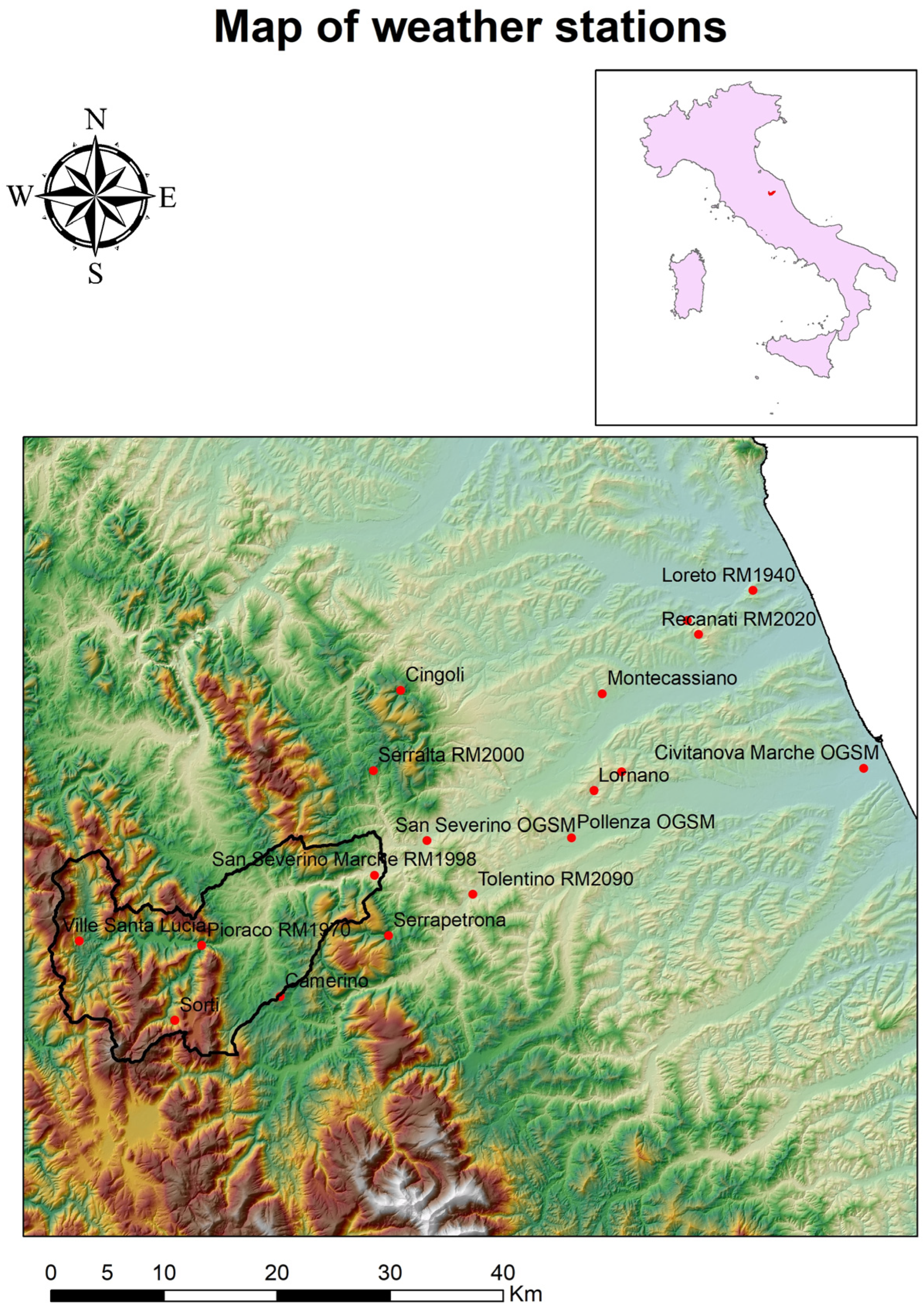
Hydrometric data, obtained at the hydrometric closure station located in San Severino Marche (Figure 1) and retrieved from 1964 to 1979 from the Italian Institute for Environmental Protection and Research (ISPRA) and from 2005 to 2020 from the Meteorological and Hydrological Information System service of the Marche Region, were required for this analysis. These study periods were chosen because they represent the range of existence of the hydrometric station, which was not active from 1980 to 2004. As far as climate data is concerned, instead, 16 weather stations were taken into consideration (Camerino, Cingoli, Loreto, Lornano, Macerata, Montecassiano, Pioraco, Pollenza, Recanati OGSM, Recanati, San Severino Marche OGSM, San Severino Marche, Serralta, Serrapetrona, Sorti, Tolentino), in order to prepare interpolations based on a good number of values to provide accurate estimates for both study periods (1964–1979 and 2005–2020). All weather stations considered were active during the two study periods with continuous data of precipitation and temperatures and were also prevalidated upon by the institutions managing them. Subsequently, the 16 weather stations used were validated following the tests prescribed by the WMO (World Meteorological Organization) and homogenised using the SNHT test [41,42]. (Figure 2).
It was first checked using the land use map for 1990 and that for 2018, to verify as we already knew that land use has not changed significantly in the study area. The Corine Land Cover (CLC) is a land-use inventory that began in 1985 and which, by means of satellite tracking, has made it possible to keep track of changes over the years to the present day. In this case, two maps were compared, one relating to CLC 1990 and one relating to CLC 2018, and the variation between land-use classes was also assessed graphically over the study area. In addition, the population in the study area in 1971 and in 2021 was also counted, using ISTAT (Italian National Statistical Institute) data, in order to assess whether the area can indeed be considered to be free of significant disturbances between 1964–1979 and 2005–2020 that could influence the measured flow rates in one direction or another. The second step was to interpolate the rainfall, in order to obtain monthly and annual averages for both study periods, in the research area. The most suitable interpolative method was cokriging with altitude as the independent variable, since after a prior analysis of the correlation between precipitation and altitude in the area, Pearson correlation coefficients between 0.63 and 0.81 were found for both study periods, which were high enough to guarantee excellent results. In this case, ordinary cokriging (OCK) (1) was used instead of simple cokriging, as the assumption that the mean is known over the entire area being interpolated, cannot be considered correct due to the non-pervasive coverage of the area, because of the low number of weather stations present.
Z O C K ( u ) = α 1 = 1 n 1 ( u ) λ α 1 O C K ( u ) Z 1 ( u α 1 ) + α 2 = 1 n 2 ( u ) λ α 2 O C K ( u ) Z 1 ( u α 2 )
Z ( u ) = primary variable
λ α = kriging weight for the α primary data sample
In order to be able to assess the goodness of an interpolative method, the cross-validation procedure with the one-leave-out method was used, which resulted in four statistical indices: mean standardized error (MSE), root mean square error standardized (RMSSE), root mean square error (RMSE) and average standard error (ASE) [43].
Root Mean Square Error (RMSE) (2), is the standard deviation between observed and predicted values. This parameter allows an assessment of the prediction errors for different weather stations; however, RMSE is not an absolute parameter, since it is impossible to compare different variables with the RMSE, but only the same dataset. The value of RMSE should be the smallest possible and similar to the ASE (average standard error), in this way, when it is predicting a value in a point without observation points it has only the ASE to assess the uncertainty of the prediction:
RMSE = i = 1 n [ Z ^ ( s i ) z ( s i ) ] 2 n
    z ^ ( s i ) = estimated value
z ( s i ) = observed value
n = sample size
Average Standard Error (ASE) (3)–this statistical tool is known also as the standard deviation from the mean and it is used to estimate the standard deviation of a sampling distribution. The ASE is an estimator of the bias of the RMSE (i.e., the standard deviation of the estimation error), a value close to zero and similar to RMSE represents a very low error in the estimation of the variability of the sampling distribution:
ASE = i = 1 n σ ^ 2 ( s i ) n
Mean Standardized Error (MSE) (4) is similar to the mean error and calculates the difference between measured and predicted values; however, the MSE values are not related to single variables but can be used to compare different variables. The standardization procedure leads a variable with mean x and variance σ2, to another with mean zero and variance equal to 1, in order to allow comparison between different variables. The mean standardized error is represented by the ratio between the mean absolute error and the standard deviation of the estimation error:
MSE = i = 1 n   [ Z ^ ^ ( s i ) z ( s i ) ] / σ ^ ( s i ) n
σ ^ ( s i ) = standard deviation
Root Mean Square Standardized Error (RMSSE) (5 allows the assessment of the efficacy of prediction models, it is desirable to have a value close to 1. If the value of RMSSE is lower than 1 the variability is overestimated, otherwise, it is underestimated; this is a dimensionless statistical tool, independent from the considered variable and it is the most significant instrument to evaluate the interpolative model with other variables:
RMSSE = i = 1 n   [ Z ^ ( s i ) z ( s i ) / σ ^ ( s i ) ] 2 n
The effective precipitation was then calculated by subtracting the potential evapotranspiration from the precipitation, estimated with Turc’s Equation (6) using the average annual precipitation and the average annual temperature (7) for each study period [44].
E T p   ( m m a n n o ) = P 0.9 + P 2 L 2
  L = 300 + 25 T + 0.05 T 3
    P = average annual precipitation
T = average annual temperature
In addition, the presence of a trend was tested for both effective precipitation and evapotranspiration by means of the Mann–Kendall test (MK), with the slope calculated through Sen’s slope estimator method. The Mann–Kendall (8) test makes no assumptions about the underlying distribution of the data and its rank-based measure is not affected by extreme value. Instead, Sen’s slope corresponds to the median of all calculated slopes between each pair of points in the series. The Mann–Kendall test was used by setting an alpha value of 0.05, i.e., with a 95% confidence level, thus the test is meaningful if the p-value is less than 0.05, meaning that one can accept the alternative hypothesis H1 and discard the null hypothesis H0.
Then the MK rank statistic dk was given by:
d k = i = 1 n p i   2 k n
Under the null hypothesis of no trend, the statistic dk is distributed as a normal distribution with the expected value of E(dk) (9) and the variance var(dk) (10) as follows:
E [ d k ] = k ( k 1 ) 4
V a r [ d k ] = k ( k 1 ) ( 2 k + 5 ) 72                 2 k n
Under the above assumption, the definition of the statistic index Zk (11) is calculated as:
Z k = d k E [ d k ] v a r [ d k ]   k = 1 , 2 , 3 , . , n
Finally, through a scatterplot and Pearson’s correlation coefficient, the correlation and linear trend were assessed for each of the two study periods.

3. Results

3.1. Verification of Land Use Change

Land use was tested by analysing the macro-categories of the CLC, both for the year 1990 and for the year 2018, and as can be seen, graphically there are no major differences (Figure 3).
In order to be even more precise and accurate, the land use percentages for both maps are given below, highlighting that the differences are absolutely minimal and not significant for the purposes of our research: 2.2% artificial surfaces CLC 2018; 37.6% agricultural areas CLC 2018; 60.2% Forest and seminatural areas CLC 2018; 1,6% artificial surfaces CLC 1990; 39.5% agricultural areas CLC 1990; and 58.9 Forest and seminatural areas CLC 1990. Finally, in order to exclude any further disturbance to our analysis, the population of the municipalities even partially affected by the study area, i.e., the upper basin of the Potenza River, was taken into account. The inhabitants of all municipalities with a portion of territory in the study area, in 1971 and 2021, were counted. The result was that in 1971, the population of the municipalities affected by the study area was 74,020 inhabitants, while the population updated to 2021 is 70,838 inhabitants, so basically there has been a decrease in population that is basically on a par with the higher water consumption at the present time.

3.2. Interpolation of Precipitation

Watershed management requires data related to the very important issue of precipitation, often measured with rain gauges. The reliability of spatialization is determined by the quality of the precipitation distribution within the study area, which derives primarily from data quality control [45] and secondarily from interpolation. Several geostatistical interpolation methods were tested for precipitation in the upper Potenza basin, but the best, based on the cross-correlation results, obtained by the one-leave-out method, was ordinary cokriging. Table 1 and Table 2 show that all the statistical indices have values very close to the optimum, zero for the MSE, one for the RMSSE and similar values between RMSE and ASE.
The results of the interpolations are monthly average values over the upper basin of the river Potenza (Table 3), which allows the analysis to continue until the actual rainfall and river flows are correlated. It is evident from Table 3 there is a difference in terms of average monthly precipitation over the basin, between the period 1964–1979 and the period 2005–2020. In particular, the biggest differences in percentages are in the months of September, October and August.
Taking the annual period into consideration, the rainfall analysis shows two different trends, one decreasing for the period 1964–1979 and the other increasing for the period 2005–2020 (Figure 4). In each case, the Mann–Kendall test on the trend shows p-values that do not allow the null hypothesis of no significant trend to be rejected. Interpolation was then performed for both periods, of which the experimental semivariogram is reported (Figure 5).
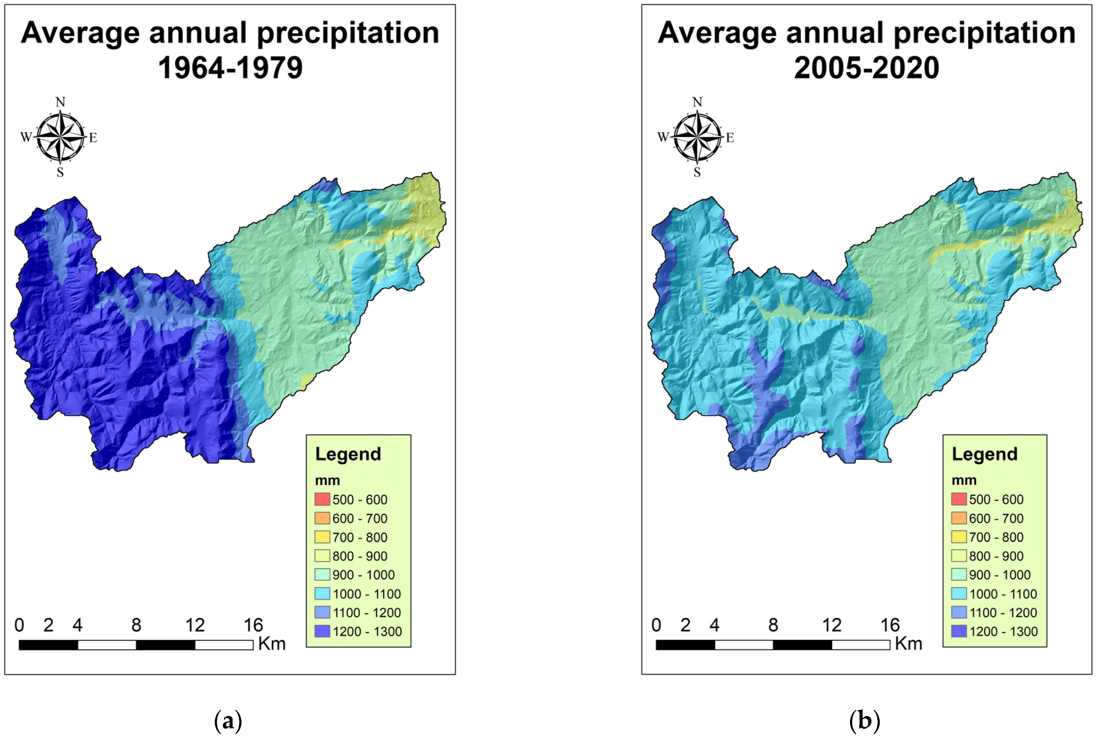
Analysing the average annual rainfall by interpolating the values of the two periods shows that there are some differences between the two periods, approximately 100 mm less rainfall for the period 2005–2020, 1153 mm for the period 1964–1979 and 1023 mm for the period 2005–2020 (Figure 6).
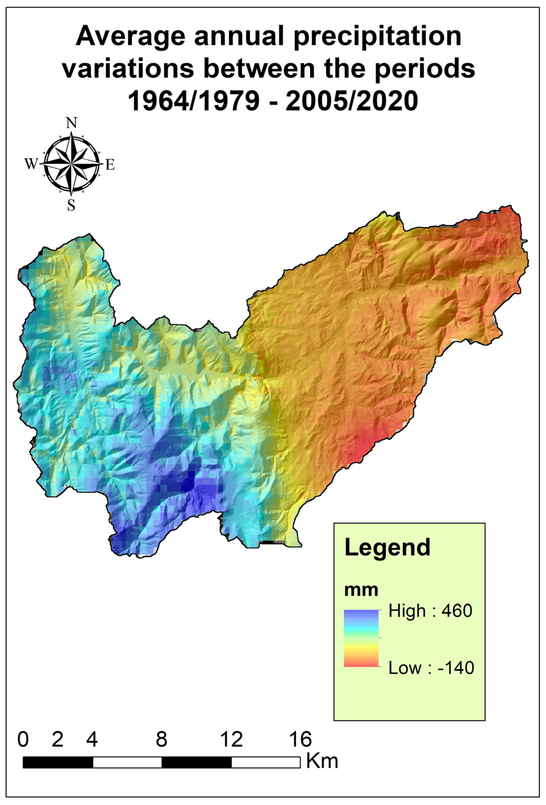
A difference map was then made between the two rasters in Figure 6 and a marked decrease in rainfall, especially in the mountainous area, emerged, while in the less elevated zone, there are also increases in precipitation over the period 2005–2020 (Figure 7).

3.3. Evapotranspiration

Evapotranspiration plays a crucial role in the water balance and consequently also in streamflows. In recent times, because of the increase in temperatures due to anthropogenic global warming, the value of evapotranspiration tends to be an important variable, in assessing the water supply to vegetation and also the hydrology of a given area. Turc’s formula, similar to many other formulas that calculate evapotranspiration, has a strong dependence on temperature, hence it was necessary to interpolate temperatures in the study area for both study periods before calculating potential evapotranspiration. The interpolation of the mean annual temperatures is shown here, which is very significant for the assessment of climate change in the study area (Figure 8).
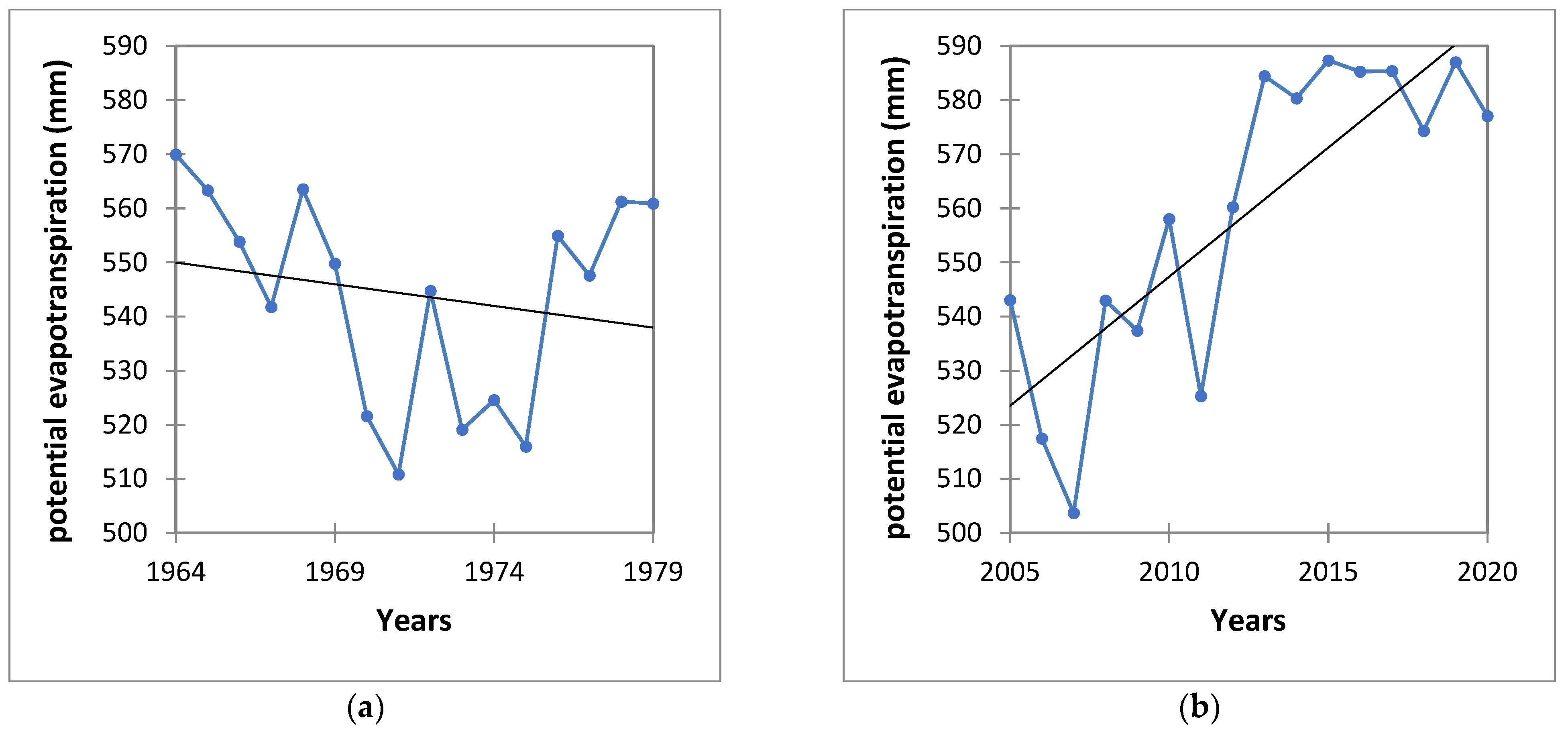
In particular, the analysis showed that the average temperature in the study area from 1964 to 1979 was 12.2 °C, while from 2005 to 2020 it was 12.9 °C, an increase of a remarkable 0.7 °C. The correctness of the interpolation of the mean annual temperatures is evidenced by the results of the cross-validation, which showed RMSSE values of 0.98 and 1.00 for the period 1964–1979 and the period 2005–2020, respectively, MSE of −0.07 and −0.09, RMSE of 0.58 and 0.57, and ASE of 0.62 and 0.59. The interpolative method used was always cokriging with altitude as the independent variable, and in this case, we can see that the relationship between the two variables is even stronger than in the case of precipitation. In this research, Turc’s formula for potential evapotranspiration showed that the increase in temperature between the two periods results in an increase in evapotranspiration of 544 mm for the period 1964–1979, and 559 mm for the period 2005–2020. As far as the trend, there is no significant 95% trend for the period 1964–1979, while the trend is significant for the period 2005–2020 with a Sen’s slope equal to 4.4 mm/year, which is so high that it results in an increase in potential evapotranspiration of 70 mm (Figure 9).

3.4. Streamflow Trend and Effective Rainfall Trend

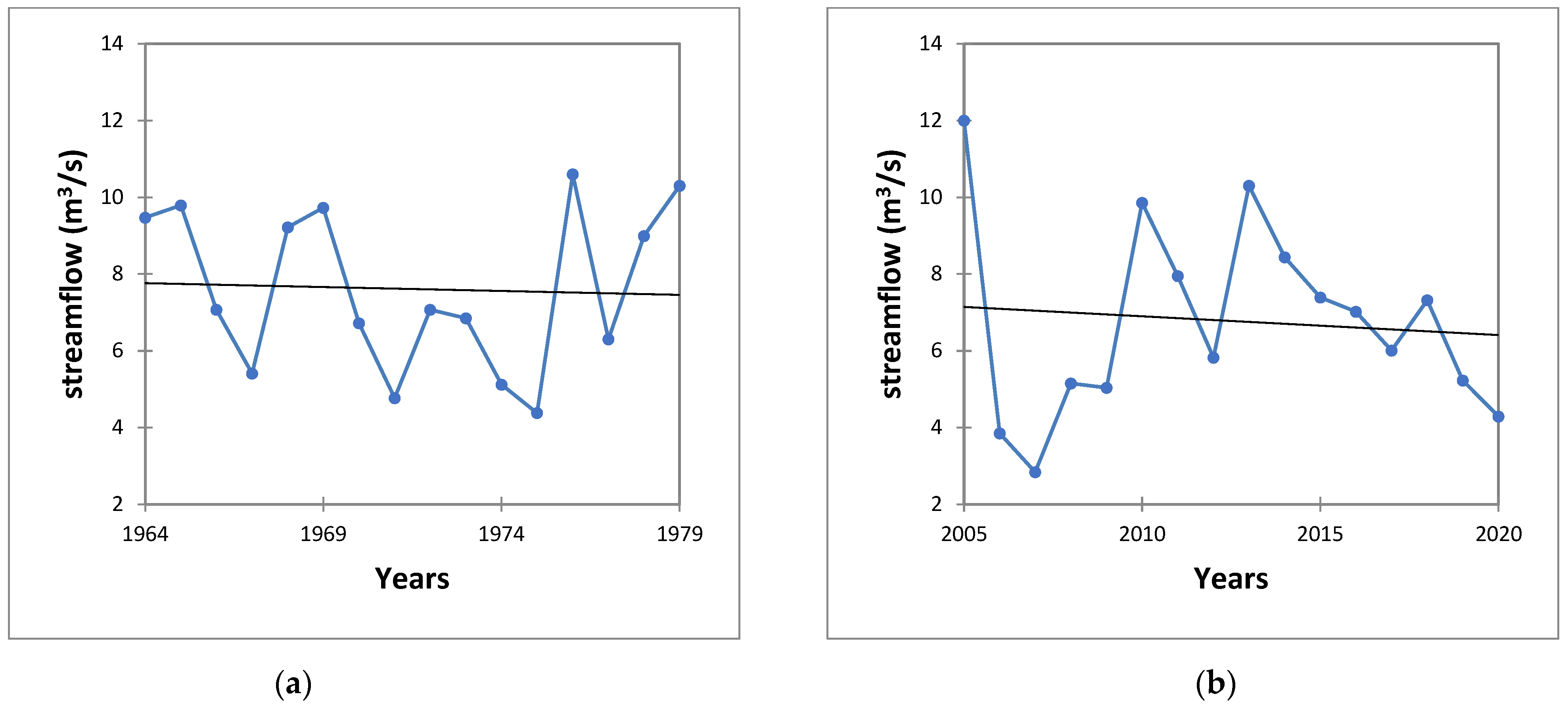
From 1964 to 1979 the minimum streamflow recorded at the San Severino Marche hydrometer station in the Potenza River was 3.757 m3/s, and the maximum streamflow was 12.166 m3/s, while the mean average streamflow of the river was 7.594 m3/s (Figure 9). The Mann–Kendall test for annual streamflow shows a decreasing trend, and Sen’s slope test also indicates a decreasing trend in annual streamflow of magnitude −0.046 m3/year (Table 4).
The period from 2005 to 2020 shows an average value of 6.730 m3/s. As can be seen in Figure 10, there is a non-significant decreasing trend in the current streamflow. The magnitude of Sen’s slope is −0.082 m3/year, which indicates a decreasing trend (Table 4).
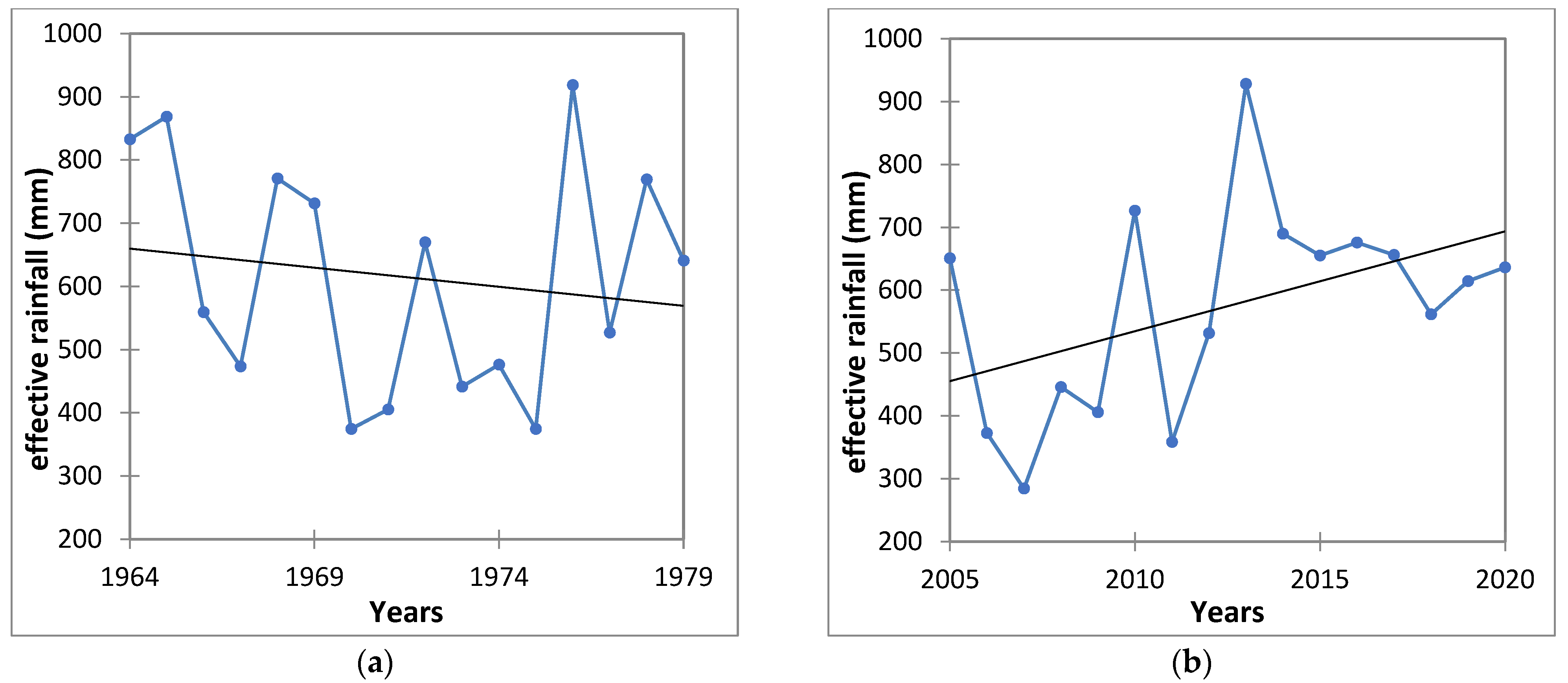
The effective precipitation amplifies the differences between the two periods observed in the average precipitation, as Figure 11 shows; furthermore the effective precipitation trend is summarised in Table 5. Again, as in the case of discharge, rainfall is very different and the trend is downward, but not significant.
The trends of the effective precipitation turn out to be very similar to those of the streamflow, at least on a first graphical analysis for the period 1964–1979, whereas, in the period 2005–2020, the trend is opposite (Figure 11). Although the trend is opposite and therefore suggests an increase in actual precipitation, this is actually not the case since precipitation increases due to higher values from 2013 onwards. If we analyse the averages of the two periods, we note that the period 1964–1979 has an average actual precipitation of 615 mm, while for the period 2005–2020, the actual precipitation is 575 mm. This result would assume in the subsequent streamflow analysis that the flow rate could be lower in the period 2005–2020 than in the period 1964–1979 if the effective precipitation amounts were respected and showed a good correlation with the streamflow.

3.5. Analysis of the Relationship between Streamflow and Effective Precipitation and Averages of the Analysed Parameters

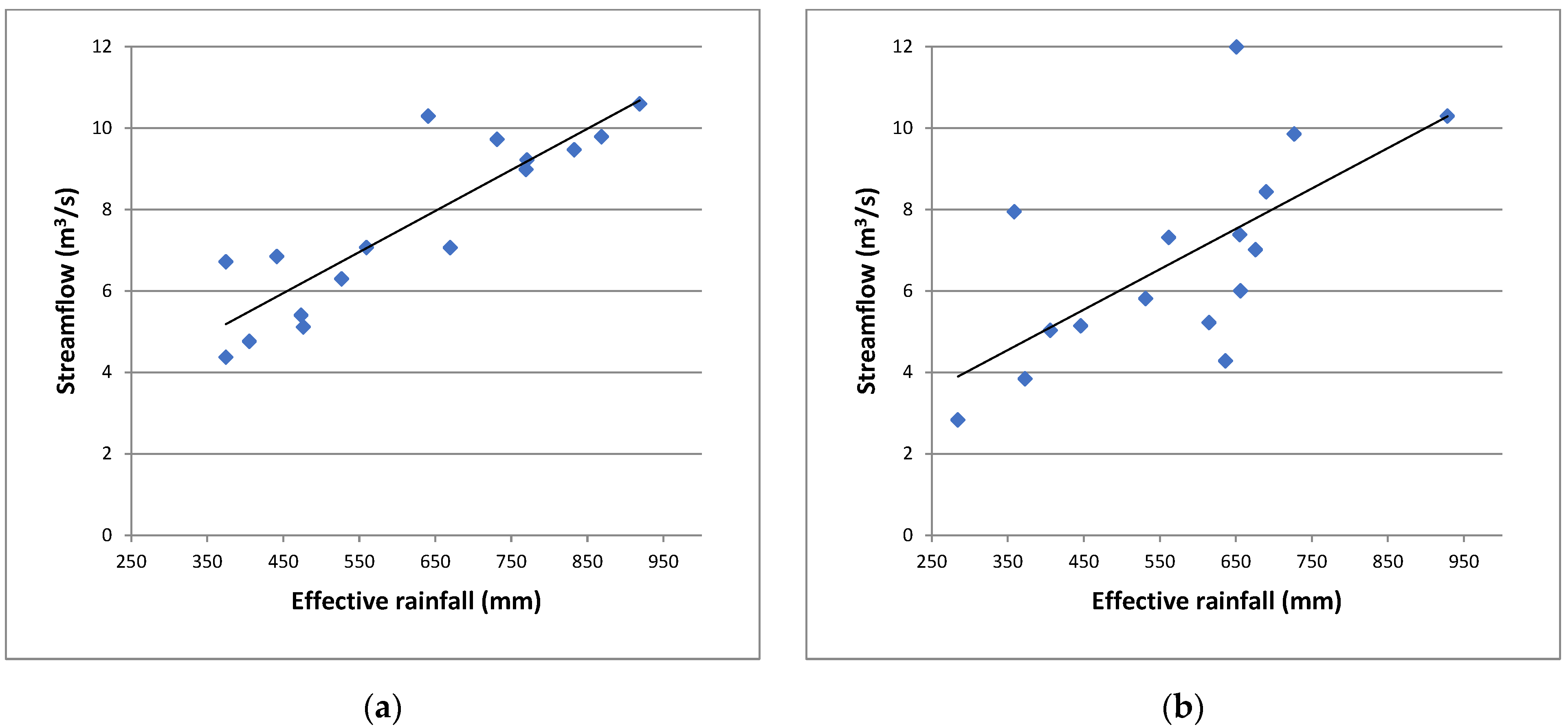
Primarily, the correlation between streamflow and effective precipitation was tested to assess whether the trend was in agreement. The correlation between streamflow and effective precipitation showed very high values for both periods, 0.798 for the period 1964–1979 and 0.776 for the period 2005–2020 (Figure 12). Thus, the correlation is positive and very similar for both periods, despite the mutual differences in precipitation values.
This testifies to the invariability of the correlations between flow rates and effective rainfall in the absence of anthropogenic abstraction even at different times, despite ongoing climate change. To enable a better understanding and reproducibility of the research, the table (Table 6) shows the averages of all parameters calculated for both study periods (1964–1979 and 2005–2020).

4. Discussion

This research has highlighted the possibility of analysing streamflows within a small basin, as a function of climatic variables subject to anthropisation-induced changes. It has been shown repeatedly by various researchers that flow rates are influenced and thus dependent on climatic variables, in particular temperature and precipitation [46]. The evidence of streamflows and precipitation in this study is a weakly decreasing trend that has been observed in other areas of the world [47], although this trend does not appear to be unambiguous, as exactly opposite trends have been observed in other locations [46]. However, flow trends can also be strongly influenced by the exploitation of the water resource, which can introduce disturbances that induce errors in the assessment of climate change and its relationship to flow rates [48]. For this reason, special attention was paid in this research to the absence of current and past exploitation of the water resource, thus only the upstream part of the basin was analysed, a part that is known and demonstrated through land use maps and population variations that has not been subject to substantial changes in anthropogenic water abstraction. In the literature on the subject, there is a tendency to favour surveys that are very extensive from a spatial point of view and rather general in their assessment of the system, whereas in this case an attempt was made to cleanse the flow data of other influences that may be purely natural, although not necessarily climatic. In addition, in order to assess the precipitation over the analysed portion of the basin, several rain gauges were taken, which allowed interpolations to be carried out; in this case using geostatistical kriging methods, in particular taking into account the strong correlation with altitude (used as an independent variable), hence cokriging was performed. Cokriging is a statistical technique that is gaining increasing popularity in the scientific literature for the interpolation of precipitation, often using very different independent variables depending on the correlation in the specific area of analysis [49]. In this context, the results of the present interpolation allow us to understand with certainty, given the excellent value of the statistical indicators, MSE, RMSE, RMSSE and ASE, the amount of annual precipitation in the basin. Several international studies have also analysed precipitation within catchments using this method; however, these interpolations have often led to poorer results in some months than those obtained in this research [50]. The estimation of potential evapotranspiration in this research was carried out using Turc’s method, because it is one of the most reliable and widely used for this estimation and has been found in numerous studies on the subject [51]. The subtraction of the potential evapotranspiration from the rainfall interpolation calculated on the upper course of the Potenza River basin provided the effective rainfall value, which is indispensable for correlating it with the flow data. Very often in the scientific literature, there is a tendency to correlate flow rates only with rainfall [52,53], neglecting the temperature-related component of climate change that could increase evapotranspiration and consequently decrease the water available for the river in a given basin, as in this case. In particular, it was interesting to note that although the effective precipitation has an increasing trend for the period 2005–2020 and a decreasing trend for the period 1964–1979, it is nevertheless lower on average in the period 2005–2020, which results in lower precipitation in the latter period and a direct relationship with the streamflow very similar in terms of ratio to the period 1964–1979. In conclusion, the results of this research show that the relationship between streamflow, precipitation and temperature in the same reservoir tends to remain constant, although, in the context of climate change, the quantities may vary, as also demonstrated in this study. The constancy of the relationship between streamflow and precipitation can hardly ever be verified by international studies, as it is subjected to the perturbations of the anthropogenic part, which is very influential over rather long periods and does not allow the contributions of one or the other component to be accurately divided [54]. Much more often though, there is a tendency to assess on the basis of a reference period and emission scenarios, the evolution of flow rates does not help operational management of the water resource in the short term [55].

5. Conclusions

The primary aim of this study is to promote a methodology for analysing the time series of river flows in relation to climatic variables. In particular, it is of interest to assess the influence of climate change on river flows, by interpolating precipitation and calculating potential evapotranspiration, in order to obtain values as close as possible to the amount of water that annually falls on the reservoir under investigation. This research aims to create a methodology for analysis, but also to assess a basin with particular attention to the changes it may have undergone over the years in terms of outflows, trying as far as possible to choose parts of the reservoir without anthropic effects, thus analysing changes due only to climate change. This operational method is aimed at understanding the influence of climate change on river flows in small watersheds, as was completed for the pilot area where two periods almost 30 years apart in time were compared, with no problems of human-induced changes. It would be interesting in the future to find watersheds or parts of them that can be considered free of man-made effects, by evaluating the correlations between climate and precipitation, in order to obtain the actual influences between climate and river flows for very large areas, and consequently to evaluate any flow changes under different emission scenarios much more accurately. Currently, in order to assess the impact of anthropogenic development on hydrology, there is fervent scientific research aimed at defining models that can simulate past land use in the light of present land use, creating a hydrometeorological model that can provide data corrected to remove anthropogenic impact [56].

Author Contributions

Conceptualization, M.G., S.I.D. and Y.H.; methodology, M.G. and S.I.D.; software, S.I.D.; validation, G.P. and M.B.; formal analysis, M.G.; investigation, S.I.D.; resources, M.G.; data curation, M.G.; writing—original draft preparation, M.G.; writing—review and editing, G.P. and M.B.; visualization, S.I.D.; supervision, G.P. and M.B.; project administration, M.G.; All authors have read and agreed to the published version of the manuscript.

Funding

This research received no external funding.

Data Availability Statement

Not applicable.

Conflicts of Interest

The authors declare no conflict of interest.

References

  1. Döll, P.; Fiedler, K.; Zhang, J. Global-scale analysis of river flow alterations due to water withdrawals and reservoirs. Hydrol. Earth Syst. Sci. 2009, 13, 2413–2432. [Google Scholar] [CrossRef]
  2. Mengistu, D.; Bewket, W.; Dosio, A.; Panitz, H.J. Climate change impacts on water resources in the upper blue nile (Abay) river basin, ethiopia. J. Hydrol. 2021, 592, 125614. [Google Scholar] [CrossRef]
  3. Feng, X.; Zhang, G.; Yin, X. Hydrological responses to climate change in Nenjiang river basin, northeastern China. Water Res. Manag. 2011, 25, 677–689. [Google Scholar] [CrossRef]
  4. Kundzewicz, Z.W.; Kanae, S.; Seneviratne, S.I.; Handmer, J.; Nicholls, N.; Peduzzi, P.; Mechler, R.; Bouwer, L.M.; Arnell, N.; Mach, K.; et al. Le risque d’inondation et les perspectives de changement climatique mondial et régional. Hydrol. Sci. J. 2014, 59, 1–28. [Google Scholar] [CrossRef]
  5. Oki, T.; Kanae, S. Global hydrological cycles and world water resources. Science 2006, 313, 1068–1072. [Google Scholar] [CrossRef] [PubMed]
  6. Tao, H.; Gemmer, M.; Bai, Y.; Su, B.; Mao, W. Trends of streamflow in the Tarim River Basin during the past 50 years: Human impact or climate change? J. Hydrol. 2011, 400, 1–9. [Google Scholar] [CrossRef]
  7. Binder, L.C.W. Climate Change and Watershed Planning in Washington State 1. J. Am. Water Res. Assoc. 2006, 42, 915–926. [Google Scholar] [CrossRef]
  8. Barnett, T.P.; Adam, J.C.; Lettenmaier, D.P. Potential impacts of a warming climate on water availability in snow-dominated regions. Nature 2005, 438, 303–309. [Google Scholar] [CrossRef]
  9. Chiew, F.H.; McMahon, T.A. Global ENSO-streamflow teleconnection, streamflow forecasting and interannual variability. Hydrol. Sci. J. 2002, 47, 505–522. [Google Scholar] [CrossRef]
  10. Dai, A.; Qian, T.; Trenberth, K.E.; Milliman, J.D. Changes in continental freshwater discharge from 1948 to 2004. J. Clim. 2009, 22, 2773–2792. [Google Scholar] [CrossRef]
  11. Fu, G.; Barber, M.E.; Chen, S. Hydro-climatic variability and trends in Washington State for the last 50 years. Hydrol. Process. 2010, 24, 866–878. [Google Scholar] [CrossRef]
  12. Nohara, D.; Kitoh, A.; Hosaka, M.; Oki, T. Impact of climate change on river discharge projected by multimodel ensemble. J. Hydrometeorol. 2006, 7, 1076–1089. [Google Scholar] [CrossRef]
  13. Vogl, A.L.; Lopes, V.L. Impacts of water resources development on flow regimes in the Brazos River. Environ. Monit. Assess. 2009, 157, 331–345. [Google Scholar] [CrossRef] [PubMed]
  14. Hannah, D.M.; Demuth, S.; van Lanen, H.A.; Looser, U.; Prudhomme, C.; Rees, G.; Stahl, K.; Tallaksen, L.M. Large-scale river flow archives: Importance, current status and future needs. Hydrol. Process. 2011, 25, 1191–1200. [Google Scholar] [CrossRef]
  15. Marsh, T.J. Capitalising on river flow data to meet changing national needs—A UK perspective. Flow Meas. Instrum. 2002, 13, 291–298. [Google Scholar] [CrossRef]
  16. Stahl, K.; Hisdal, H.; Hannaford, J.; Tallaksen, L.M.; van Lanen, H.A.J.; Sauquet, E.; Demuth, S.; Fendekova, M.; Jódar, J. Streamflow trends in Europe: Evidence from a dataset of near-natural catchments. Hydrol. Earth Syst. Sci. 2010, 14, 2367–2382. [Google Scholar] [CrossRef]
  17. Rojas, R.; Feyen, L.; Bianchi, A.; Dosio, A. Assessment of future flood hazard in Europe using a large ensemble of bias-corrected regional climate simulations. J. Geophys. Res. Atmos. 2012, 117, D17109. [Google Scholar]
  18. Blöschl, G.; Hall, J.; Viglione, A.; Perdigão, R.A.P.; Parajka, J.; Merz, B.; Lun, D.; Arheimer, B.; Aronica, G.T.; Bilibashi, A.; et al. Changing climate both increases and decreases European river floods. Nature 2019, 573, 108–111. [Google Scholar] [CrossRef]
  19. Blöschl, G.; Gaál, L.; Hall, J.; Kiss, A.; Komma, J.; Nester, T.; Parajka, J.; Perdigão, R.A.P.; Plavcová, L.; Rogger, M.; et al. Increasing river floods: Fiction or reality? Wiley Interdiscip. Rev. Water 2015, 2, 329–344. [Google Scholar] [CrossRef]
  20. Gentilucci, M.; Barbieri, M.; Burt, P. Climate and territorial suitability for the Vineyards developed using GIS techniques. In Proceeding of the Conference of the Arabian Journal of Geosciences; Springer: Cham, Switzerland, 2018; pp. 11–13. [Google Scholar]
  21. Reidsma, P.; Ewert, F.; Lansink, A.O.; Leemans, R. Adaptation to climate change and climate variability in European agriculture: The importance of farm level responses. Eur. J. Agron. 2010, 32, 91–102. [Google Scholar] [CrossRef]
  22. Gentilucci, M.; Moustafa, A.A.; Abdel-Gawad, F.K.; Mansour, S.R.; Coppola, M.R.; Caserta, L.; Inglese, S.; Pambianchi, G.; Guerriero, G. Advances in Egyptian mediterranean coast climate change monitoring. Water 2021, 13, 1870. [Google Scholar] [CrossRef]
  23. Gentilucci, M.; Parisi, C.; Coppola, M.R.; Majdoubi, F.Z.; Madonna, A.; Guerriero, G. Influence of mediterranean sea temperature increase on Gaeta Gulf (Tyrrhenian Sea) biodiversity. Proc. Zool. Soc. 2021, 74, 91–103. [Google Scholar] [CrossRef]
  24. Antonetti, G.; Gentilucci, M.; Aringoli, D.; Pambianchi, G. Analysis of landslide Susceptibility and Tree Felling Due to an Extreme Event at Mid-Latitudes: Case Study of Storm Vaia, Italy. Land 2022, 11, 1808. [Google Scholar] [CrossRef]
  25. Bračko, T.; Žlender, B.; Jelušič, P. Implementation of Climate Change Effects on Slope Stability Analysis. Appl. Sci. 2022, 12, 8171. [Google Scholar] [CrossRef]
  26. Gentilucci, M.; Barbieri, M.; Materazzi, M.; Pambianchi, G. Effects of Climate Change on Vegetation in the Province of Macerata (Central Italy). In Advanced Studies in Efficient Environmental Design and City Planning; Springer: Cham, Switzerland, 2021; pp. 463–474. [Google Scholar]
  27. Theurillat, J.P.; Guisan, A. Potential impact of climate change on vegetation in the European Alps: A review. Clim. Chang. 2001, 50, 77–109. [Google Scholar] [CrossRef]
  28. Fagerberg, J.; Laestadius, S.; Martin, B.R. The triple challenge for Europe: The economy, climate change, and governance. Challenge 2016, 59, 178–204. [Google Scholar] [CrossRef]
  29. Gentilucci, M.; D’Aprile, F. Variations in trends of temperature and its influence on tree growth in the Tuscan Apennines. Arab. J. Geosci. 2021, 14, 1418. [Google Scholar] [CrossRef]
  30. Lionello, P.; Scarascia, L. The relation between climate change in the Mediterranean region and global warming. Reg. Environ. Chang. 2018, 18, 1481–1493. [Google Scholar] [CrossRef]
  31. Gorguner, M.; Kavvas, M.L. Modeling impacts of future climate change on reservoir storages and irrigation water demands in a Mediterranean basin. Sci. Total Environ. 2020, 748, 141246. [Google Scholar] [CrossRef]
  32. Javadian, M.; Behrangi, A.; Smith, W.K.; Isher, J.B. Global trends in evapotranspiration dominated by increases across large cropland regions. Remote Sens. 2020, 12, 1221. [Google Scholar] [CrossRef]
  33. Yue, T.X.; Zhao, N.; Ramsey, R.D.; Wang, C.L.; Fan, Z.M.; Chen, C.F.; Lu, Y.M.; Li, B.L. Climate change trend in China, with improved accuracy. Clim. Chang. 2013, 120, 137–151. [Google Scholar] [CrossRef]
  34. Bhutiyani, M.R.; Kale, V.S.; Pawar, N.J. Climate change and the precipitation variations in the northwestern Himalaya: 1866–2006. Int. J. Climatol. 2010, 30, 535–548. [Google Scholar] [CrossRef]
  35. Tabari, H. Climate change impact on flood and extreme precipitation increases with water availability. Sci. Rep. 2020, 10, 13768. [Google Scholar] [CrossRef] [PubMed]
  36. Grazzini, F.; Craig, G.C.; Keil, C.; Antolini, G.; Pavan, V. Extreme precipitation events over northern Italy. Part I: A systematic classification with machine-learning techniques. Q. J. R. Meteorol. Soc. 2020, 146, 69–85. [Google Scholar] [CrossRef]
  37. Gentilucci, M.; Barbieri, M.; D’Aprile, F.; Zardi, D. Analysis of extreme precipitation indices in the Marche region (central Italy), combined with the assessment of energy implications and hydrogeological risk. Energy Rep. 2020, 6, 804–810. [Google Scholar] [CrossRef]
  38. Cheng, L.; AghaKouchak, A. Nonstationary precipitation intensity-duration-frequency curves for infrastructure design in a changing climate. Sci. Rep. 2014, 4, 7093. [Google Scholar] [CrossRef]
  39. Olmstead, S.M. Climate change adaptation and water resource management: A review of the literature. Energy Econ. 2014, 46, 500–509. [Google Scholar] [CrossRef]
  40. Brandolini, P.; Cevasco, A.; Firpo, M.; Robbiano, A.; Sacchini, A. Geo-hydrological risk management for civil protection purposes in the urban area of Genoa (Liguria, NW Italy). Nat. Hazards Earth Syst. Sci. 2012, 12, 943–959. [Google Scholar] [CrossRef]
  41. Aguilar, E.; Auer, I.; Brunet, M.; Peterson, T.C.; Wieringa, J. Guidance on Metadata and Homogenization; WMOv (World Meteorological Organization): Geneva, Switzerland, 2003. [Google Scholar]
  42. Gentilucci, M.; Catorci, A.; Panichella, T.; Moscatelli, S.; Hamed, Y.; Missaoui, R.; Pambianchi, G. Analysis of Snow Cover in the Sibillini Mountains in Central Italy. Climate 2023, 11, 72. [Google Scholar] [CrossRef]
  43. Goovaerts, P. Ordinary Cokriging Revisited. Math. Geol. 1998, 30, 21–42. [Google Scholar] [CrossRef]
  44. Turc, L. Calcul du bilan de l’eau évaluation en fonction des précipitations et des températures. IAHS Publ. 1954, 37, 88–200. [Google Scholar]
  45. Gentilucci, M.; Barbieri, M.; Burt, P.; D’Aprile, F. Preliminary data validation and reconstruction of temperature and precipitation in Central Italy. Geosciences 2018, 8, 202. [Google Scholar] [CrossRef]
  46. Novotny, E.V.; Stefan, H.G. Stream flow in Minnesota: Indicator of climate change. J. Hydrol. 2007, 334, 319–333. [Google Scholar] [CrossRef]
  47. Esvandzibaie, F.; Farajzadeh, M.; Ghavidel, Y. Analysis of temporal and spatial changes of precipitation and flow rate in arid regions with a statistical approach (case study: Central Plateau catchment area of Iran). Int. J. Environ. Sci. Technol. 2022, 19, 6803–6824. [Google Scholar] [CrossRef]
  48. Ortega, J.A.; Razola, L.; Garzón, G. Recent human impacts and change in dynamics and morphology of ephemeral rivers. Nat. Hazards Earth Syst. Sci. 2014, 14, 713–730. [Google Scholar] [CrossRef]
  49. Usowicz, B.; Lipiec, J.; Łukowski, M.; Słomiński, J. Improvement of spatial interpolation of precipitation distribution using cokriging incorporating rain-gauge and satellite (SMOS) soil moisture data. Remote Sens. 2021, 13, 1039. [Google Scholar] [CrossRef]
  50. Adhikary, S.K.; Muttil, N.; Yilmaz, A.G. Cokriging for enhanced spatial interpolation of rainfall in two Australian catchments. Hydrol. Process. 2017, 31, 2143–2161. [Google Scholar] [CrossRef]
  51. Dimitriadou, S.; Nikolakopoulos, K.G. Annual actual evapotranspiration estimation via GIS models of three empirical methods employing remotely sensed data for the peloponnese, Greece, and comparison with annual MODIS ET and pan evaporation measurements. ISPRS Int. J. Geo-Inf. 2021, 10, 522. [Google Scholar] [CrossRef]
  52. Zhang, Q.; Singh, V.P.; Sun, P.; Chen, X.; Zhang, Z.; Li, J. Precipitation and streamflow changes in China: Changing patterns, causes and implications. J. Hydrol. 2011, 410, 204–216. [Google Scholar] [CrossRef]
  53. Han, H.; Hou, J.; Huang, M.; Li, Z.; Xu, K.; Zhang, D.; Xu, K.; Zhang, D.; Bai, G.; Wang, C. Impact of soil and water conservation measures and precipitation on streamflow in the middle and lower reaches of the Hulu River Basin, China. Catena 2020, 195, 104792. [Google Scholar] [CrossRef]
  54. Santos, R.M.B.; Fernandes, L.S.; Moura, J.P.; Pereira, M.G.; Pacheco, F.A.L. The impact of climate change, human interference, scale and modeling uncertainties on the estimation of aquifer properties and river flow components. J. Hydrol. 2014, 519, 1297–1314. [Google Scholar] [CrossRef]
  55. Schnorbus, M.; Werner, A.; Bennett, K. Impacts of climate change in three hydrologic regimes in British Columbia, Canada. Hydrol. Process. 2014, 28, 1170–1189. [Google Scholar] [CrossRef]
  56. Ceppi, A.; Gambini, E.; Lombardi, G.; Ravazzani, G.; Mancini, M. (SOL40: Forty Years of Simulations under Climate and Land Use Change. Water 2022, 14, 837. [Google Scholar] [CrossRef]
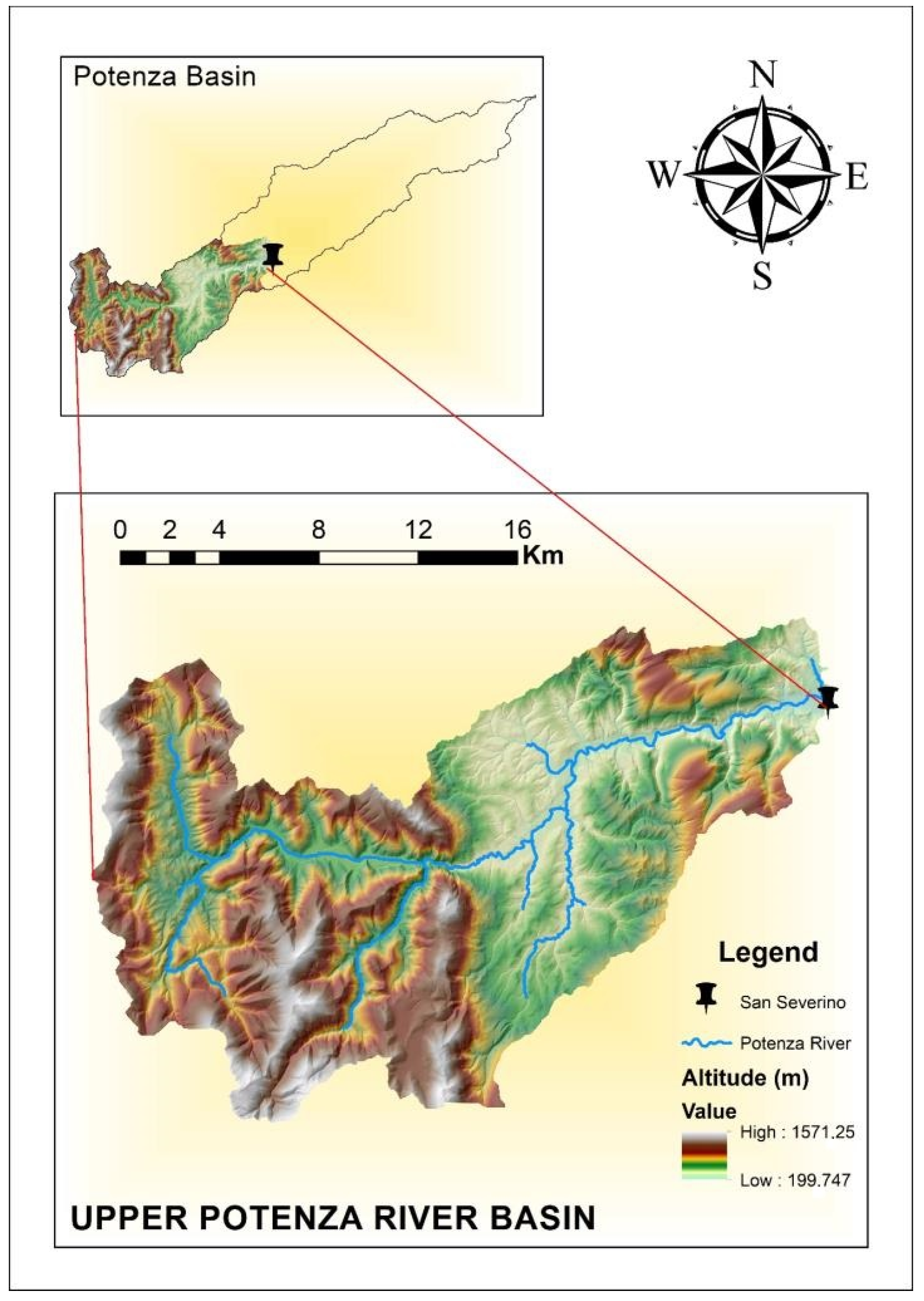
Figure 1. Geography of the study area, upper part of Potenza river basin.
Water 15 01586 g001
Figure 2. Map of weather stations.
Water 15 01586 g002
Figure 3. Corinne Land Cover, land use map: (a) CLC 1990, (b) CLC 2018.
Water 15 01586 g003
Figure 4. Annual average precipitation, in black the trend line: (a) 1964–1979; (b) 2005–2020.
Water 15 01586 g004
Figure 5. Semivariogram of the annual average precipitation: (a) 1964–1979; (b) 2005–2020. On the y-axis there is the semi-variance, while the x-axis shows the distance between pairs of observations.
Water 15 01586 g005
Figure 6. Average annual precipitation: (a) 1964–1979; (b) 2005–2020.
Water 15 01586 g006
Figure 7. Variation in average annual precipitation between the periods 1964–1979 and 2005–2020.
Water 15 01586 g007
Figure 8. Average annual temperature: (a) 1964–1979; (b) 2005–2020.
Water 15 01586 g008
Figure 9. Potential evapotranspiration and trend line in black colour: (a) 1964–1979; (b) 2005–2020.
Water 15 01586 g009
Figure 10. Streamflow and trend line in black colour: (a) 1964–1979; (b) 2005–2020.
Water 15 01586 g010
Figure 11. Effective rainfall and trend line in black colour: (a) 1964–1979 (b) 2005–2020.
Water 15 01586 g011
Figure 12. Scatter plots showing relationship between effective precipitation and streamflow, trend line in black colour: (a) 1964–1979 (b) 2005–2020.
Water 15 01586 g012
Table 1. Cross-validation statistics for monthly precipitation in the upper Potenza River basin from 1964 to 1979, MSE: mean standardized error, RMSSE: root mean square error standardized, RMSE: root mean square error, ASE: average standard error.
MonthMSERMSSERMSEASE
January−0.0340.9420.8623.35
February−0.0120.9523.3526.43
March−0.0310.9423.7926.60
April−0.0220.9524.8627.36
May−0.0290.9426.1829.45
June−0.0450.9819.9220.53
July−0.0280.9522.1623.96
August−0.0300.9618.5319.28
September−0.0710.9427.7329.60
October−0.0240.8724.6628.71
November−0.0781.0124.8024.37
December−0.0280.9227.1730.95
Table 2. Cross-validation statistics for monthly precipitation in the upper Potenza River basin from 2005 to 2020, MSE: mean standardized error, RMSSE: root mean square error standardized, RMSE: root mean square error, ASE: average standard error.
MonthMSERMSSERMSEASE
January−0.0120.8920.0623.26
February−0.0510.9326.2129.45
March−0.0610.9735.1841.35
April−0.0540.9430.2735.16
May−0.0420.9025.0729.46
June−0.0291.0231.0334.77
July−0.0061.0930.1229.84
August0.0030.9423.1124.86
September−0.0711.0235.6134.81
October−0.0210.9929.7633.30
November−0.0450.9629.2333.93
December−0.0541.0035.6238.21
Table 3. Results of monthly precipitation interpolations averaged over the upper Potenza River basin.
MonthPrec. 1964–1979Prec. 2005–2020
January82.675.5
February93.576.6
March95.1115.7
April103.983.5
May82.682.9
June88.979.9
July72.949.1
August117.772.5
September111.889.5
October92.790.2
November107.4112.5
December104.095.2
Annual1158.61133.9
Table 4. Mann-Kendall and Sen’s slope test results for streamflow trend.
PeriodKendall’s Taup-ValueSen’s Slope (m3/Year)
1964–1979−0.0920.620−0.051
2005–2020−0.0500.825−0.078
Table 5. Mann–Kendall and Sen’s slope test results for effective precipitation trend.
PeriodKendall’s Taup-ValueSen’s Slope (m3/Year)
1964–1979−0.050−0.822−1.807
2005–2020−0.0670.753−2.395
Table 6. Table comparing the averages of the variables used for the analysis over the two study periods (1964–1979; 2005–2020): P = precipitation (mm); T = temperature (°C); ETp = evapotranspiration (mm); ER = effective rainfall (mm); Q = streamflow (m3/s).
PeriodPTETpERQ
1964–1979115912.25446157.6
2005–2020113413.25595756.8
Disclaimer/Publisher’s Note: The statements, opinions and data contained in all publications are solely those of the individual author(s) and contributor(s) and not of MDPI and/or the editor(s). MDPI and/or the editor(s) disclaim responsibility for any injury to people or property resulting from any ideas, methods, instructions or products referred to in the content.