Article

New Optimized Equal-Area Mesh Used in Axisymmetric Models for Laminar Transient Flows

by
Pedro Leite Ferreira
1,* and
Dídia Isabel Cameira Covas
2
1
Department of Civil Engineering, Polytechnic of Porto, 4249-015 Porto, Portugal
2
CERIS, Instituto Superior Técnico, Universidade de Lisboa, 1049-001 Lisboa, Portugal
*
Author to whom correspondence should be addressed.
Water 2023, 15(7), 1402; https://doi.org/10.3390/w15071402
Submission received: 1 February 2023 / Revised: 27 March 2023 / Accepted: 30 March 2023 / Published: 4 April 2023
(This article belongs to the Special Issue About an Important Phenomenon—Water Hammer)

Abstract

:
The current paper aims at assessing the effect of the radial mesh on the description of the axial velocity in steady-state and transient conditions and at presenting the results of a new optimized equal-area mesh. For this purpose, a quasi-2D model is implemented and tested for different mesh configurations and sizes. A new two-region mesh geometry with 40 cylinders is proposed to optimize the description of the wall shear stress immediately after each pressure variation. This mesh is composed of two regions: one with a high-resolution near the pipe wall and the second with a coarser grid in the pipe core. Different configurations of this mesh are analysed for both steady and unsteady conditions. Results are compared with those obtained by a 1D model and with experimental data for laminar flows, discussed in terms of the computation effort and accuracy. The proposed two-region mesh has demonstrated: (i) a reduction in the simulation error by five times when compared with standard meshes for the same computational effort and for the instantaneous valve closure; (ii) an important improvement in accuracy for an experimental S-shape valve maneuver, particularly for meshes with few cylinders; and (iii) a correct description of the transient pressures collected in the experimental tests.

1. Introduction

A hydraulic transient corresponds to an intermediate state between two stationary flows, generated by valve maneuvers, pumps or turbines. This phenomenon can occur not only in water supply systems, but also in hydropower systems, the aircraft industry, railways tunnels, etc. [1,2,3]. Hydraulic transient analysis is particularly important in the design stage of pressurized systems in order to specify the pipe material and wall thickness, and, whenever necessary, to design surge protection devices.
Classic transient analysis, considering steady-state friction formulas (amongst other assumptions), is commonly used for design purposes, as it describes the maximum and minimum pressure variations reasonably well [2,3,4]. However, these models cannot accurately represent the complete transient phenomenon due to the wave propagation and complex diffusion mechanisms that significantly affect the pressure wave dissipation, dispersion and shape. This is particularly relevant in fast and high-frequency transient events, in which unsteady friction has a dominant effect [5,6]. Several efforts have been made to develop models with more accurate, simpler and lower computational demands, and the description of energy dissipation in pressurized transient flows has been a major challenge over the past decades; these models can be one-dimensional (1D), two-dimensional (2D) and three dimensional (3D) models, as briefly described in the following paragraphs.
In 1D models, several formulations have been proposed to compute unsteady friction for both laminar [5,7,8,9] and turbulent flows [10,11,12,13,14,15]. These formulations can be classified as instantaneous acceleration-based [16,17,18] or convolution-based [5,9,14,19,20,21,22]. Acceleration-based approaches introduce an additional term relating the local and the convective acceleration to the momentum equation. This formulation is quick to compute, but has a low accuracy; some formulations (e.g., [16,17,18]) must be calibrated based on experimental results. Convolution-based formulations consider the complete history of the local acceleration. This approach is consistent and theoretically more robust, but is very time-consuming, which is why several approximate solutions have been developed (e.g., [12,20,22]).
Axisymmetric models, also referred as quasi-two-dimensional models (Q2D), have been traditionally considered a good compromise between accuracy and computational time [6,23]. Q2D models have demonstrated consistency, regarding the physics of the phenomenon, and numerical robustness, ensuring the calculation of energy dissipation with high accuracy. More efficient versions than that initially proposed by Vardy and Hwang [6] have also been developed [24,25,26,27]. A second promising feature is the enhanced definition of the radial grid, which can ensure higher accuracy simulations with fewer cylinders and reduced computation time.
Finally, tri-dimensional computational fluid dynamics (3D-CFD) models, integrating turbulent models, are the most powerful and comprehensive hydraulic analysis models in pressurized pipes, though extremely computationally expensive in terms of time and data storage for regular use in engineering practice [28,29,30,31,32].
In any numerical model (1D, Q2D or 3D-CFD), the mesh size and configuration strongly affects the computational effort, as well as the accuracy of the results [6,33]. Not so intuitive, but equally important, is that the mesh must adapt to geometrical boundaries and to the flow physics to ensure that the velocity variation is of the same order along the numerical mesh. In practice, a non-uniform grid should be generated, with a higher resolution near the pipe wall, due to the high gradients observed. Calibrating the grid according to the velocity gradient history can reduce the number of mesh points at the same accuracy level [34]. Q2D models have a high potential for future improvements, particularly as concerns the mesh definition and optimization to be used in engineering practice.
This paper aims at the assessment of radial mesh influence on the computation of unsteady energy dissipation in pressurized pipes using a Q2D model. An extensive numerical analysis of the effect of the numerical schemes and of the radial mesh on the computation of unsteady energy is carried out. Several radial meshes are defined, as a compromise between flow dynamics and total mesh points. A comprehensive analysis and comparison of the Q2D results obtained with experimental data with results from 1D model are conducted for laminar flows and for two valve closure maneuvers (i.e., an instantaneous and a S-shape closure).
The key innovative features of the current paper are: (i) the analysis of a new optimized equal-area mesh (divided into high and low-resolution regions) applying transient laminar flows created by an instantaneous valve closure; (ii) the application of the new mesh to transient tests observed in an experimental facility, created by a S-shaped valve closure; and (iii) the assessment of the advantages of neglecting the lateral velocity transfer for both instantaneous and calibrated valve maneuvers.

2. Numerical Models

2.1. The Vardy and Hwang (1991) Model: Basic Equations, Assumptions and Numerical Scheme

The Q2D model makes the same traditional 1D model assumptions concerning the fluid and the pipe, namely: (i) the fluid is one-phase, homogenous, almost incompressible and isothermal (i.e., fluid properties—density and viscosity—are constant); and (ii) the pipe is uniform, is completely constrained from any axial or lateral movement and has linear-elastic rheological behavior. The axisymmetric flow assumptions allow neglect of the radial velocity and the viscous terms not perpendicular to the flow, simplifying the momentum equation in the conduit direction—Equation (1)—and eliminating the radial momentum equation. Consequently, the pressure is constant in the radial direction (the reason why axisymmetric models are also referred to as quasi-2D models). The governing equations constitute a system of two partial differential equations with three unknown parameters (p, u , υ ) with the following form [6,24]:
H t + c 2 g u x = c 2 g r ( r υ ) r
1 g u t + H x = 1 r ρ r 𝜏 r
𝜏 = ρ ν u r
where x is the distance along the pipe; r is the distance from the axis in the radial direction; t is time; H is the piezometric head; u (x, r, t) is the local axial velocity; υ (x, r, t) is the local radial velocity; g is the gravitational acceleration; c is the wave speed; ρ is the liquid density; 𝜏 is the shear stress; and ν is the liquid kinematic viscosity.
The Q2D model divides the pipe radial section into NC concentric and hollow cylinders, extended along the whole pipe length (Figure 1). The pipe length, L, is divided into N X equal reaches, such that Δ x = L / N X , and each hollow cylinder has Δ x length. Each cylinder is defined by the respective index, j, increasing from the centerline ( j = 0 ) to the pipe wall ( j = N C 1 ). The wall thickness of the jth cylinder is denoted by Δ r j ( = r j r j 1 ), the external radius by r j ( = 0 j Δ r j ) and the cylinder center radius is r j ¯ = ( r j 1 + r j ) / 2 . The time step is determined according to the Courant condition, Δ t = Δ x / c . Each conduit section, referred to as xi, is located at a distance x = Δ x . i from the upstream end of the pipe.
The Q2D model uses the Method of Characteristics to numerically solve the axial propagation of the pressure wave in each cylinder, defined by the terms on the left-hand side of Equations (4) and (5). The terms on the right-hand side of these equations are approximated by a second-order central difference formula. Accordingly, the Q2D model equations at each cylinder are:
H i t + 1 D j θ 2 q i , j 1 t + 1 + D j θ 2 q i , j t + 1 A j θ 1 u i , j 1 t + 1 + ( a g + C j θ 1 ) × u i , j t + 1 θ 1 B j u i , j + 1 t + 1 = H i 1 t + D j × ( 1 θ 2 ) × q i 1 , j 1 t D j × ( 1 θ 2 ) × q i 1 , j t + A j × ( 1 θ 1 ) × u i 1 , j 1 t + ( a g ( 1 θ 1 ) × C j ) × u i 1 , j t + ( 1 θ 1 ) × B j × u i 1 , j + 1 t
H i t + 1 D j θ 2 q i , j 1 t + 1 + D j θ 2 q i , j t + 1 + A j θ 1 u i , j 1 t + 1 ( a g + C j θ 1 ) × u i , j t + 1 + θ 1 B j u i , j + 1 t + 1 = H i + 1 t + D j × ( 1 θ 2 ) × q i + 1 , j 1 t D j × ( 1 θ 2 ) × q i + 1 , j t A j × ( 1 θ 1 ) × u i + 1 , j 1 t ( a g ( 1 θ 1 ) × C j ) × u i + 1 , j t ( 1 θ 1 ) × B j × u i + 1 , j + 1 t
A j = { 0   ; j = 0 c Δ t ν j 1 r j ¯   Δ r j g × r j 1 ( r j ¯ r j 1 ¯ )   ; j > 0
B j = { c Δ t ν j r j ¯   Δ r j + 1 g × r j r j + 1 ¯ r j ¯   ;   j < N C 1 c Δ t ν j r j ¯   Δ r j + 1 g × r j r j + 1 ¯ r j ¯   ; j = N C 1
C j = A j + B j
D j = c 2 Δ t g × 1 r j ¯   Δ r j
where q is the lateral mass transfer ( q = r υ ); θ 1 and θ 2 are the weighting coefficients ( θ 1 and θ 2 vary between 0 and 1, while θ 1 + θ 2 = 1 ); subscripts i and j are the conduit grid point and radial grid point, respectively; and t refers to the time.
The general central difference formula truncation error is given by:
( ω r ) j = ω j + 1 ω j 1 r j + 1 r j 1 Δ r j + 1 Δ r j 2 × ( 2 ω r 2 ) j Δ r j + 1 2 + Δ r j + 1 . Δ r j + Δ r j 2 6 × ( 3 ω r 3 ) j T r u n c a t i o n   e r r o r
This formula is second-order accuracy, O ( Δ r 2 ) , if the variation of the grid size is very small ( Δ r j + 1 Δ r j ) and, consequently, the first term of the truncation error tends to zero. In a general non-uniform scheme, the second-order central difference scheme loses one order of accuracy and the truncation error is O ( Δ x ) . The main conclusion is that, generally, different formulas can lose at least one order of accuracy in non-uniform grids.

2.2. The Complete Zhao and Ghidaoui (2003) Model

The original Vardy and Hwang (1991) [6] model is numerically inefficient, since it requires the inversion of a (2NC × 2NC) sparse matrix. Zhao and Ghidaoui (2003) [24] proposed an improved higher efficiency numerical model, developed by algebraic manipulation of Equations (3) and (4) into two smaller systems with tridiagonal matrices. The use of tridiagonal matrices allows the use of a faster form of Gaussian elimination, named the Thomas algorithm [35]. This algorithm obtains the solution via NC operations instead of NC 3 operations needed by the original Vardy and Hwang (1991) model, where NC is the matrix dimension.
A tridiagonal system is defined and allows elimination of the piezometric-head and mass transfer from the coefficient matrix, A u , and unknown vector, z u , at time t + 1 by subtracting Equations (4) to (5) for each cylinder.
A u × z u = b u
The axial velocities matrix, A u , for each cylinder at time t + 1 is described as follows:
A u = ( 2 × ( a g + θ 1 C j = 0 ) 2 θ 1 B j = 0 a g a g a g a g a g a g a g a g 2 A j θ 1 a g a g 2 × ( a g + θ 1 C j ) a g a g 2 θ 1 B j a g a g 2 A j = N c θ 1 a g a g a g 2 × ( a g + θ 1 C j = N c ) )
The z u = ( u i , j = 0 t + 1 ,…,   u i , j t + 1 ,…,…,   u i , j = N C t + 1 ) is the axial velocities’ unknown vector. The result vector, b u , at time t depends on the piezometric head, axial velocities and lateral mass transfer and is defined as follows:
b u = { H i 1 t H i + 1 t + ( a g ( 1 θ 1 ) × C j ) × u i 1 , j t + ( a g ( 1 θ 1 ) × C j ) × u i + 1 , j t + ( 1 θ 1 ) × B j × u i 1 , j + 1 t + ( 1 θ 1 ) × B j × u i + 1 , j + 1 t D j × ( 1 θ 2 ) × q i 1 , j t + D j × ( 1 θ 2 ) × q i + 1 , j t H i 1 t H i + 1 t + A j × ( 1 θ 1 ) × u i 1 , j 1 t + A j × ( 1 θ 1 ) × u i + 1 , j 1 t + ( a g ( 1 θ 1 ) × C j ) × u i 1 , j t + ( a g ( 1 θ 1 ) × C j ) × u i + 1 , j t + ( 1 θ 1 ) × B j × u i 1 , j + 1 t + ( 1 θ 1 ) × B j × u i + 1 , j + 1 t + D j × ( 1 θ 2 ) × q i 1 , j 1 t D j × ( 1 θ 2 ) × q i + 1 , j 1 t D j × ( 1 θ 2 ) × q i 1 , j t + D j × ( 1 θ 2 ) × q i + 1 , j t H i 1 t H i + 1 t + A j × ( 1 θ 1 ) × u i 1 , j 1 t + A j × ( 1 θ 1 ) × u i + 1 , j 1 t + ( a g ( 1 θ 1 ) × C j ) × u i 1 , j t + ( a g ( 1 θ 1 ) × C j ) × u i + 1 , j t + D j × ( 1 θ 2 ) × q i 1 , j 1 t D j × ( 1 θ 2 ) × q i + 1 , j 1 t }
The lateral velocities and the piezometric-head are calculated by adding Equations (4) and (5) for each cylinder, and the equation obtained for the first cylinder is subtracted from the second equation and so on, obtaining the coefficient matrix, A q , and unknown vector, z q , at time t + 1.
A q × z q = b q
The mass transfer and piezometric-head coefficient matrix, A q , for each cylinder at time t + 1 is described as follows:
A q = ( a g 2 2 θ 2 D j = 0 2 . θ 2 . ( D j = n 1 D j = n 2 ) a g a g a g 2 . θ 2 . ( D j = n 1 D j = n 2 ) a g 0 a g . θ 2 . D j = 0 a g 2 θ 2 D j 1 a g 2 θ 2 × ( D j 1 + D j ) + a g 2 θ 2 D j + 2 . a g . ( a g D j = n 1 D j = n 2 ) a g a g . θ 2 . D j = 0 a g . θ 2 . D j = 0 2 . D j = N c 1 θ 2 a g + 2 . θ 2 . a g j   + 2 . a g . ( a g D j = n 1 D j = n 2 ) a g 0 a g . θ 2 . D j = 0 a g . θ 2 . D j = 0 2 . D j = N c 1 θ 2 a g a g 2 θ 2 D j = N c 2 2 θ 2 × ( D j = N c 1 D j = N c 2 ) a g )
The z q = ( H i t + 1 ,   q i , 0 t + 1 ,…,   q i , j t + 1 ,…, q i , j = N C 1 t + 1 ) is the unknown vector. The result vector, b q , depends on the piezometric-head and on the velocities (axial and lateral) at the time t and is defined by:
b q = { H i 1 t + H i + 1 t + ( a g ( 1 θ 1 ) × C j = 0 ) × ( u i 1 , j = 0 t u i + 1 , j = 0 t ) + ( 1 θ 1 ) × B j = 0 × ( u i 1 , j = 1 t u i + 1 , j = 1 t ) D j = 0 × ( 1 θ 2 ) × ( q i 1 , j = 0 t + q i + 1 , j = 0 t ) A j × ( 1 θ 1 ) × ( u i 1 , j 1 t u i + 1 , j 1 t ) A j 1 × ( 1 θ 1 ) × ( u i 1 , j 2 t u i + 1 , j 2 t ) + ( a g ( 1 θ 1 ) × C j ) × ( u i 1 , j t u i + 1 , j t ) ( a g ( 1 θ 1 ) × C j 1 ) × ( u i 1 , j 1 t u i + 1 , j 1 t ) + ( 1 θ 1 ) × B j × ( u i 1 , j + 1 t u i + 1 , j + 1 t ) ( 1 θ 1 ) × B j × ( u i 1 , j t u i + 1 , j t ) + D j . ( 1 θ 2 ) × ( q i 1 , j 1 t + q i + 1 , j 1 t q i 1 , j t q i + 1 , j t ) D j 1 × ( 1 θ 2 ) × ( q i 1 , j 2 t + q i + 1 , j 2 t q i 1 , j 1 t q i + 1 , j 1 t ) × q i + 1 , j t A j = n 1 × ( 1 θ 1 ) × ( u i 1 , j = n 2 t u i + 1 , j = n 2 t ) A j = n 2 × ( 1 θ 1 ) × ( u i 1 , j = n 3 t u i + 1 , j = n 3 t ) + ( a g ( 1 θ 1 ) × C j = n 1 ) × ( u i 1 , j = n 1 t u i + 1 , j = n 1 t ) ( a g ( 1 θ 1 ) × C j = n 2 ) × ( u i 1 , j = n 2 t u i + 1 , j = n 2 t ) ( 1 θ 1 ) × B j = n 1 × ( u i 1 , j = n 1 t u i + 1 , j = n 1 t ) + D j = n 1 × ( 1 θ 2 ) × ( q i 1 , j = n 2 t + q i + 1 , j = n 2 t q i 1 , j = n 1 t q i + 1 , j = n 1 t ) }

2.3. The Simplified Zhao and Ghidaoui (2003) Model

Usually, the radial velocity is of significantly lower magnitude than the axial velocity, thus justifying the respective elimination from Equation (1), with further computation simplifications [26]. Using the scheme of Zhao and Ghidaoui (2003) [24], the axial velocity for each cylinder is calculated by Equations (12) and (13) and the piezometric head uses the tradition 1D model discretization form of Equation (17), obtained by summing the MOC characteristics equations [2,26]. The wall shear stress is defined by the axial velocity in the wall cylinder using Equation (18) and the mean velocity is calculated by the radial velocity integration, as presented in Equation (19).
H i t + 1 = 1 2 ( H i 1 t + H i + 1 t + c g × ( U i 1 t + U i + 1 t ) ) ( 1 θ * ) × c Δ t ρ g R × ( 𝜏 w i 1 t 𝜏 w i + 1 t )
𝜏 w = μ j = N c × u j = N c R r ¯ j = N c
U = 1 S j = 0 j = N C + 1 u j Δ s j
where U is the mean velocity in the complete pipe cross section; R is the pipe radius; θ* is a weighting coefficient considered equal to 0.5, Δ s j = 2 π r ¯ j Δ r j is the cross section of each hollow cylinder, and S is the complete pipe cross section.
Additionally, neglecting the radial velocity allows the use of θ 1 = 1 in Equations (12) and (13), which further simplifies the calculation of vector z q .

2.4. Radial Mesh Discretization

The radial mesh (or grid) generation is crucial for the accurate simulation of the flow, both in steady and unsteady conditions. A computer code was implemented to allow the definition of the three traditional radial meshes (Figure 2): (i) geometric sequence cylinders (GS); (ii) equal area cylinders (EAC); and (iii) equal thickness cylinders (ETC).
The geometric sequence (GS) mesh is defined by fixing the first cylinder thickness near the pipe wall, Δ r j = N C 1 , and the geometric sequence common ratio, C R . The thickness of cylinder j is calculated as follows:
Δ r j = Δ r j = N C 1 × ( 1 + C R ) N C j
A particular GS mesh is referred to as “GS CR NC”, in which NC represents the total number of cylinders. This radial geometry has been widely used by several researchers [24,25,27].
The equal area cylinder (EAC) mesh assumes cylinders with a uniform area along the pipe radius, as follows:
Δ r j + 1 2 Δ r j 2 = c o n s t
Bratland [23] and Vardy and Hwang [6] used a mesh that is only defined by NC, that is “EAC NC”.
The equal thickness cylinder (ETC) mesh, also implemented by Vardy and Hwang [6], ensures a constant thickness of the radial grid and is also only described by the total number of cylinders, NC, as “ETC NC”, as follows:
Δ r j + 1 Δ r j = c o n s t

3. Experimental Facility Description

Transient tests for laminar flow conditions were carried out in the experimental facility assembled at the Laboratory of Hydraulics and Water Resources of the Instituto Superior Técnico (Figure 3). These tests were conducted for a discharge of 0.016 L/s, corresponding to a Reynolds number (Re = UD/ν) equal to 1000. Water was at 20 °C with a density ρ = 1000 kg/m3 and a kinematic viscosity ν = 1.01 × 10⁻⁶ m2/s.
The system has a reservoir-pipe-valve configuration, with a rigidly supported straight copper pipe with an inner diameter, D, of 20 mm, wall thickness, e, of 0.001 m and a total length, L, of 15.2 m. A centrifugal pump with a hydro-pneumatic vessel is installed at the upstream end of the pipe to simulate a constant level reservoir. Two in-line ball valves are installed at the downstream end of the pipe: one valve, manually actuated, is used to control the flow rate and the other valve, pneumatically actuated, is used to generate the transient event. Different closure times are attained by varying the operating pressure of the pneumatic valve [36].
The data acquisition system (DAS) is composed of a computer, a Picoscope 3424 oscilloscope, a trigger-synchronizer, an electromagnetic flowmeter (with a 0.4% accuracy) and two strain-gauge type pressure transducers (WIKA S-10, 25 bars nominal pressure and 0.25% full-scale span accuracy). The first transducer is at the upstream end of the ball valve and the second is at the pipe mid-length.
The experimental wave speed, c, estimated based on the travelling time of the pressure wave between the two transducers, is 1250 m/s, which is consistent with values of previous studies carried out in the same experimental facility [36,37,38,39,40,41].
The valve closure law of the ball valve was thoroughly studied by Ferreira et al. [36]. The authors concluded that, despite the valve total closure time being higher than the system characteristic time, 2L/c, the effective closure of the ball valve corresponds to 1/10 to 1/8 of the total closure time, and a rapid maneuver is always attained. The maneuver can be described by the sigmoidal-type closure law, as follows:
Q Q 0 = ( 1 1 + e ξ ( 𝜏 95 ) ) η
where 𝜏 is the valve closure percentage, and ξ and η are the coefficients that best fit the numerical results with collected pressure-head data.
In the current study, the considered manoeuvre has total and effective closure times of 0.045 and 0.005 s, respectively. Accordingly, the experimental and Q2D models’ calibrated results are presented in Figure 4. The calibrated flow rate variation is shown in Figure 4a. The piezometric head obtained in the Q2D model fits almost perfectly with the collected data (Figure 4b).

4. Numerical Results for the Instantaneous Valve Closure

4.1. Introduction

This section presents the results obtained by the Q2D model proposed by Zhao and Ghidaoui (2003) applied to an experimental pipe system for simulation of an instantaneous maneuver in a laminar flow. First, the effect of the mesh size near the pipe wall is analyzed for several standard equal area meshes, and results are compared with the reference Zielke’s solution implemented in 1D models. Secondly, results from the Q2D model with an optimized equal-area cylinder, and with 40 cylinders, are compared with those from standard equal area meshes.

4.2. Standard Equal-Area Cylinder Mesh: Effect of the Mesh Discretization

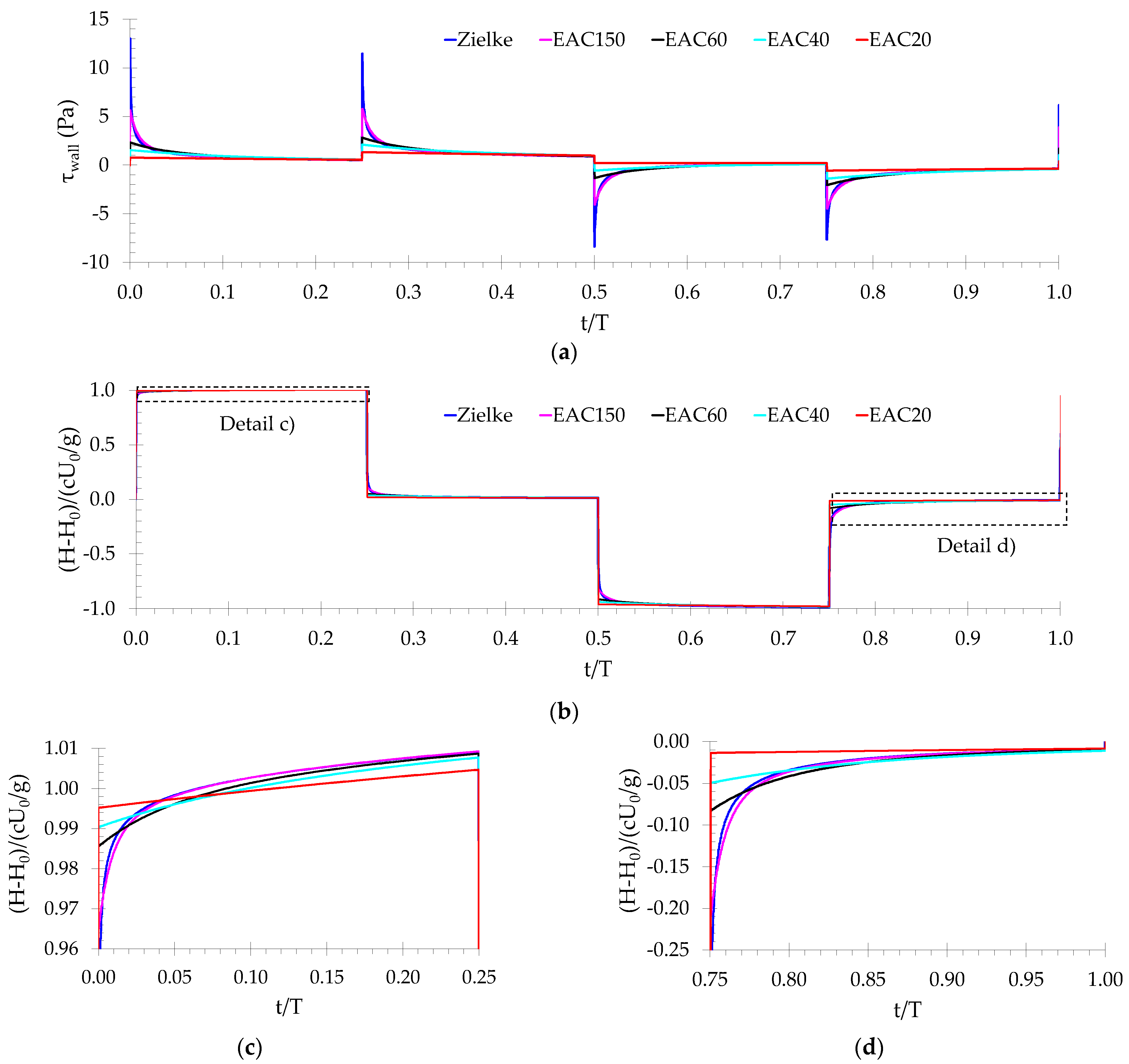
The numerical Q2D results for the wall shear stress and the piezometric-head with the standard equal-area cylinder mesh (EAC) and a variable number of cylinders (Nc = 20, 40, 60 and 150) are depicted in Figure 5. Zielke’s 1D model is also plotted in this figure and used as the benchmark solution for comparison.
The effect of the number of cylinders, NC, is observed immediately after the first pressure wave arrival. The 1D model shows a high wall shear stress peak after each pressure surge, followed by an exponential decay (Figure 5a). Low NC meshes show a lower peak and a linear decay with time. Increasing the NC value brings the Q2D model simulation closer to Zielke’s 1D solution. The NC = 20 mesh reduces the Zielke’s peak more than 17 times; the NC = 150 mesh increases the previous value almost eight times but is still approximately half the 1D model peak.
As expected, a more precise wall shear stress calculation leads to a better piezometric description. For the NC = 20 mesh, the Q2D model piezometric-head results (Figure 5b–d) do not depict the correct wave shape (the round-shape), showing a square shape geometry, and present a poor calculation of the wave damping (e.g., for t/T = 0.25, the difference to the 1D model is noticeable). Increasing the number of cylinders allows progressive approximation of Zielke’s results.
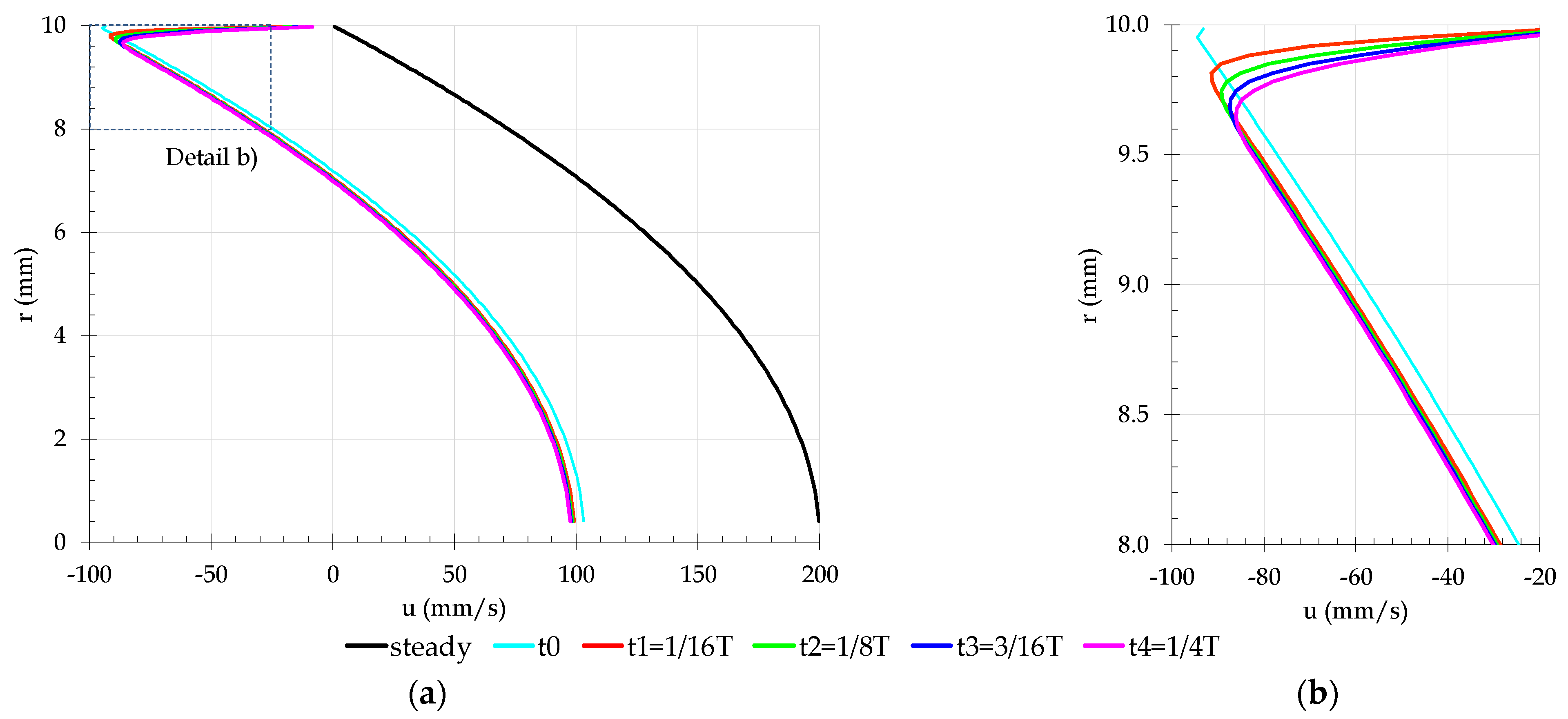
The Q2D model computes the wall shear stress and the piezometric-head at a given time based on the axial velocity calculation. Figure 6 shows the axial velocity profile for the EAC150 mesh simulation at five-time steps during the first pressure surge (0 ≤ t/T ≤ 0.25). The time steps are equally spaced: t0 is the velocity profile immediately after the pressure wave arrival, and each new time adds t/16T to the previous one (t0 = 0, t1 = t/16T, t2 = t/8T, t3 = 3/16T and t4 = 1/4T).
The pressure surge arrival shifts the steady-state axial velocity profile and an inflection point with a high axial velocity gradient appears near the pipe wall because of the no-slip condition. From t0 to t5, the velocity profile gradient near the wall reduces as the inflection point moves into the pipe core. The transient flow changes occur close to the pipe wall. At t4, just before the next pressure surge, the inflection point maximum displacement from the pipe wall is less than 4% of the pipe radius. Therefore, a high percentage of the pipe profile is unaffected and the Q2D model’s cylinders maintain a steady-state profile axial velocity.
The Q2D model numerical scheme accuracy is estimated by the finite difference truncation error, Equation (10). This means that high axial velocity variations must be followed by considerably lower grid intervals, Δ r , to achieve the same accuracy. The formation of the inflection point leads to a high numerical error in the pipe wall area and a low error in the pipe core, because it maintains the steady-state axial velocity profile with a parabolic variation ( 2 u / 2 r c o n s t a n t ). The mesh refinement should focus on the wall area where the high axial velocity variations occur.
The EAC mesh geometry uniformly reduces the grid space in the pipe section, implying a considerable computational effort to approximate the 1D model results, especially immediately after each pressure surge. The use of EAC150 mesh corresponds to almost eight times the EAC20 computational effort, as it increases linearly with the number of cylinders for the implemented numerical scheme.

4.3. Optimized Equal-Area Cylinder Mesh

4.3.1. Mesh Description

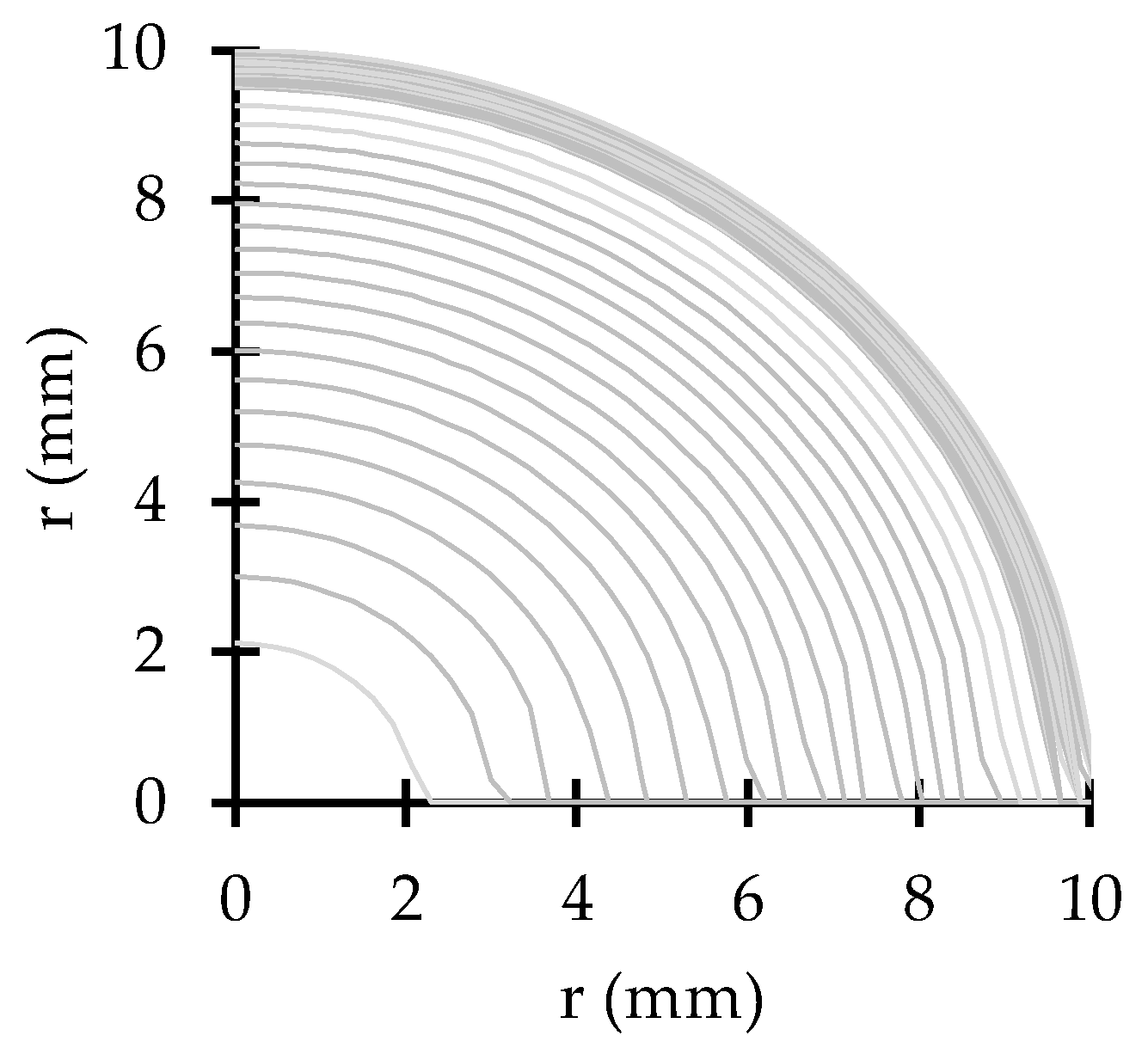
The optimized equal-area cylinder (OEAC) mesh, innovatively proposed in this research, has a high-resolution grid close to the pipe wall and a low-resolution grid in the pipe core, as presented in Figure 7. Two equal-area cylinder meshes are implemented, with the lowest cylinder area near the wall. The underlying principle is to use a finer mesh in areas with high-velocity gradients and a coarse mesh in the low-velocity gradient region, thus, reducing the computational effort.
The new mesh is characterized by three parameters: (i) the total number of cylinders, NC; (ii) the limit of the high-resolution grid, r, defined as a percentage of the pipe radius and measured from the pipe wall; and (iii) the number of cylinders in the high-resolution region, NHR. Thus, the optimized equal area cylinder (OEAC) meshes are expressed as follows, OEACNC Nr = NHR. For instances, OEAC40 N5% = 20 stands for a mesh that has a total of 40 cylinders (NC = 40); the limit of the high-resolution mesh occurs at r = 9.5 mm (r/R = 5%) and has 20 cylinders in this high-resolution region.
This mesh is referred to as optimized since it provides better results than those for the standard EAC meshes for the same number of cylinders, as demonstrated in the following sections. This analysis will be carried out for NC = 40, because the EAC mesh with 40 cylinders does not lead to an accurate simulation of the piezometric head (Figure 5b), representing a good comparison with optimized mesh.

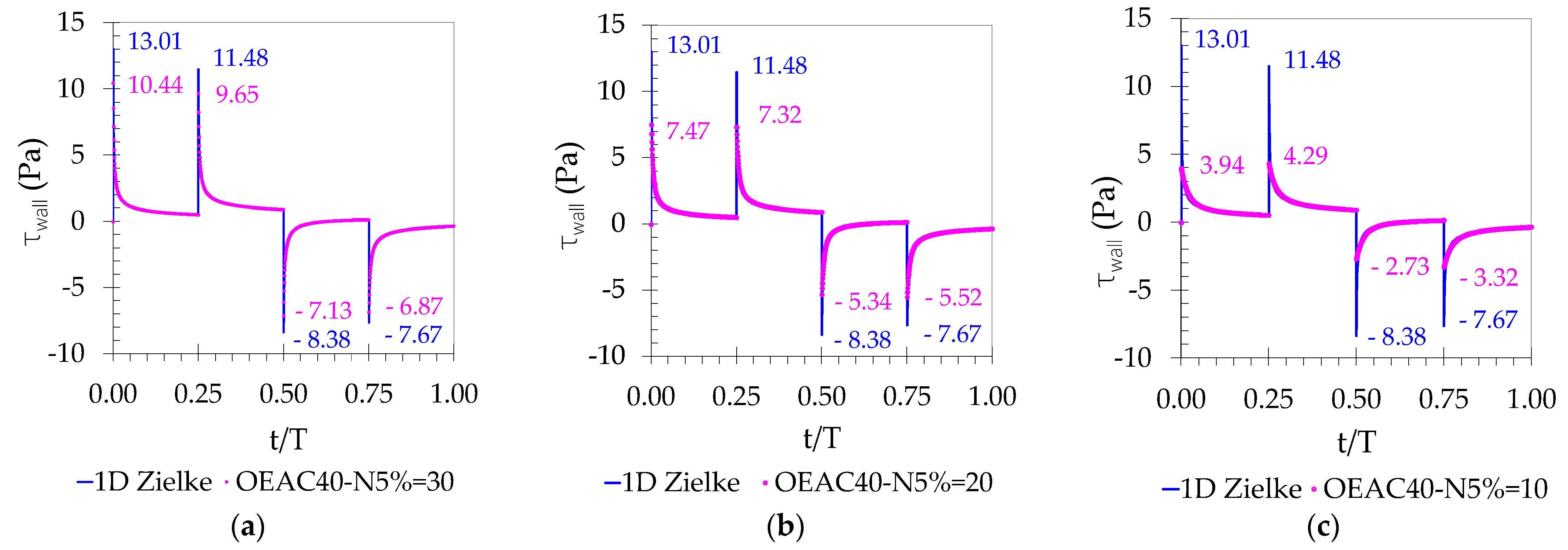
4.3.2. Shear Stress Results

The wall shear stress obtained by the Q2D model for the optimized equal-area cylinder (OEAC) meshes with NHR between 10 to 30, r = 5% and NC = 40 are presented in Figure 8. The r = 5% corresponds to the inflection point maximum displacement determined in the previous analysis (Figure 6). All simulations’ accuracy has significantly improved compared to the EAC results (Figure 4), for the same total number of cylinders (NC = 40). The new mesh with more than 20 cylinders in the wall region (OEAC40 N5% = 20) also presents better results than the 150 equal area cylinder meshes (EAC150). These results are compared with those obtained by the Zielke formulation used in the 1D model.
The OEAC40 N5% = 30 mesh allows an almost perfect adjustment to Zielke’s results (Figure 8a), whereas the OEAC40 N5% = 10 mesh leads to a maximum wall shear stress four times lower than the Zielke’s value. This shows that the higher the number of cylinders in the high-resolution area, the more accurate the prediction of the maximum wall stress and of the subsequent decay. A second aspect concerns the relation between the wall shear stress peak values in the deceleration (t/T = 0 and t/T = 0.25) and the acceleration (t/T = 0.50 and t/T = 0.75) phases. For the meshes with higher resolution near the wall (NHR ≥ 20), the peaks decay with time, as in the Zielke model; on the contrary, for the low resolution mesh (Figure 8c), the peaks increase compared with the previous surge for t/T = 0.25 and t/T = 0.75, as observed for the standard meshes (Figure 8a).
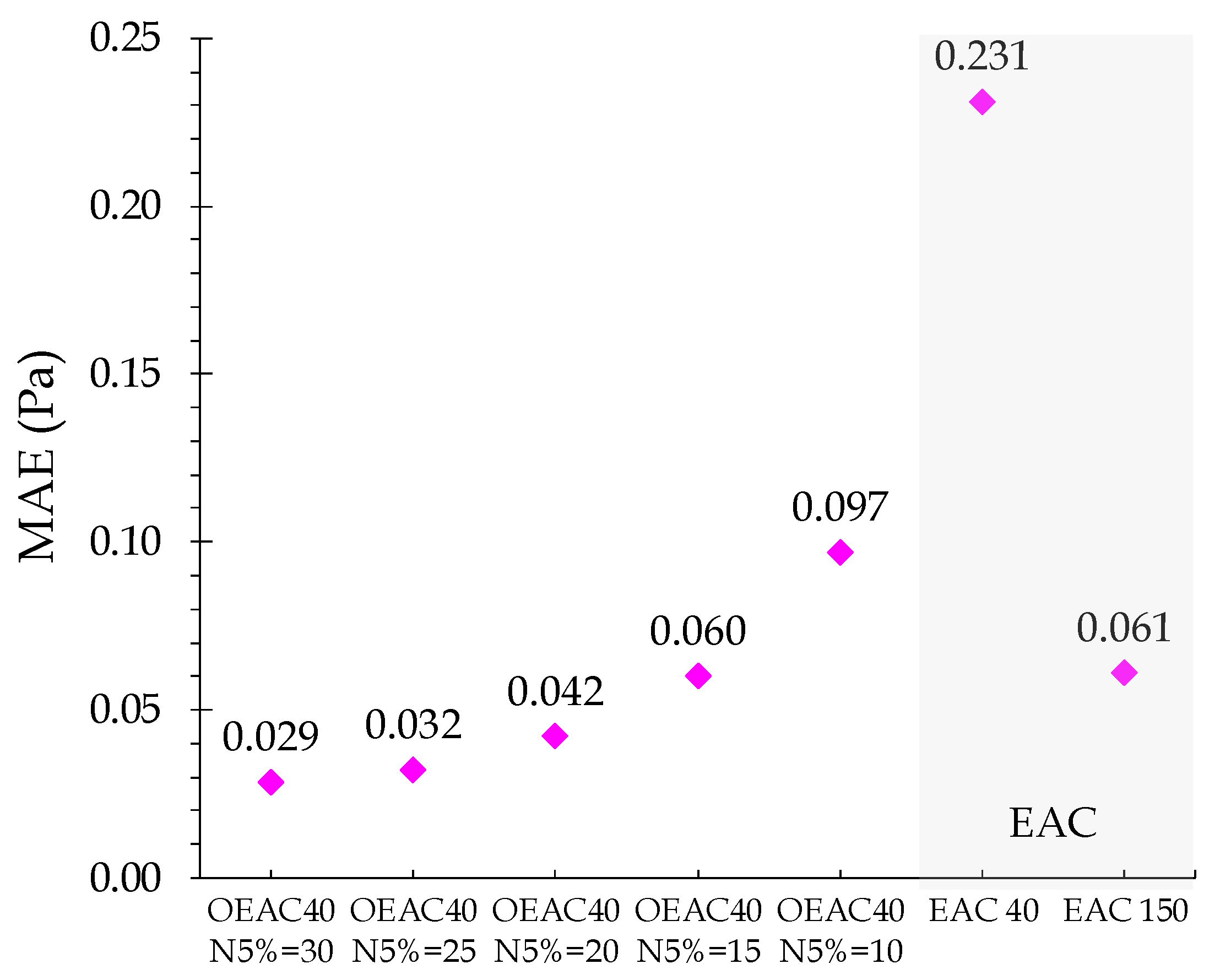
The mean absolute error (MAE) is used to measure the Q2D accuracy, using paired observation from the 1D Zielke model, and is given by:
MAE = i = 1 n | y i x i | n
in which n is the total number of time step at the pipe middle section, y is the Zielke model value (assumed as exact) and x is the Q2D predicted value, both for the same instance i.
The MAE calculation for the wall shear stress simulation during the first pressure wave period (0 < t/T ≤ 1) confirms the previous assessment (Figure 9). MAE shows an almost exponential increase along with the NHR reduction. For the same number of cylinders, the EAC40 mesh results have an error almost 10 times higher than that of the best OEAC mesh (OEAC40 N5% = 30). The EAC150 results present the same MAE as the OEAC40 N5% = 15 and a higher error than when using a higher NHR value. This analysis highlights that a higher accuracy can be achieved with one-quarter of the number of standard mesh cylinders (40/150). OEAC mesh’s results are clearly better than those obtained for the EAC grid, considering the same (EAC40), or even a higher (EAC150), value of the total number of cylinders.

4.3.3. Mean Velocity and Piezometric Head Results

The Q2D model simulation accuracy for the mean velocity and piezometric head depends not only on the unsteady wall shear stress calculation, but also on the steady-state velocity profile calculation. 
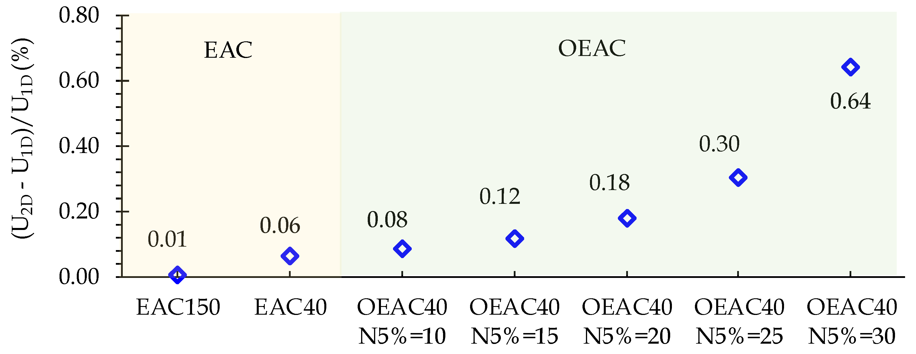
Figure 10 shows the relative steady-state mean velocity error for EAC and OEAC meshes, described by ( U 2 D U 1 D ) / U 1 D , in which U 1D is the steady-state mean velocity obtained by Hagen–Poiseuille solution and U2D is the Q2D model steady-state flow approximation for each mesh. Firstly, OEAC meshes have a worse steady-state velocity representation than the EAC meshes (i.e., the EAC40 mesh leads to a lower error). Secondly, this error increases exponentially with the NHR increase. The OEAC40 N5% = 10 mesh has a 0.08% error, which is close to EAC40 (0.06%), but the OEAC40 N5% = 30 error rises to 0.64% (i.e., 8 to 10 times higher).
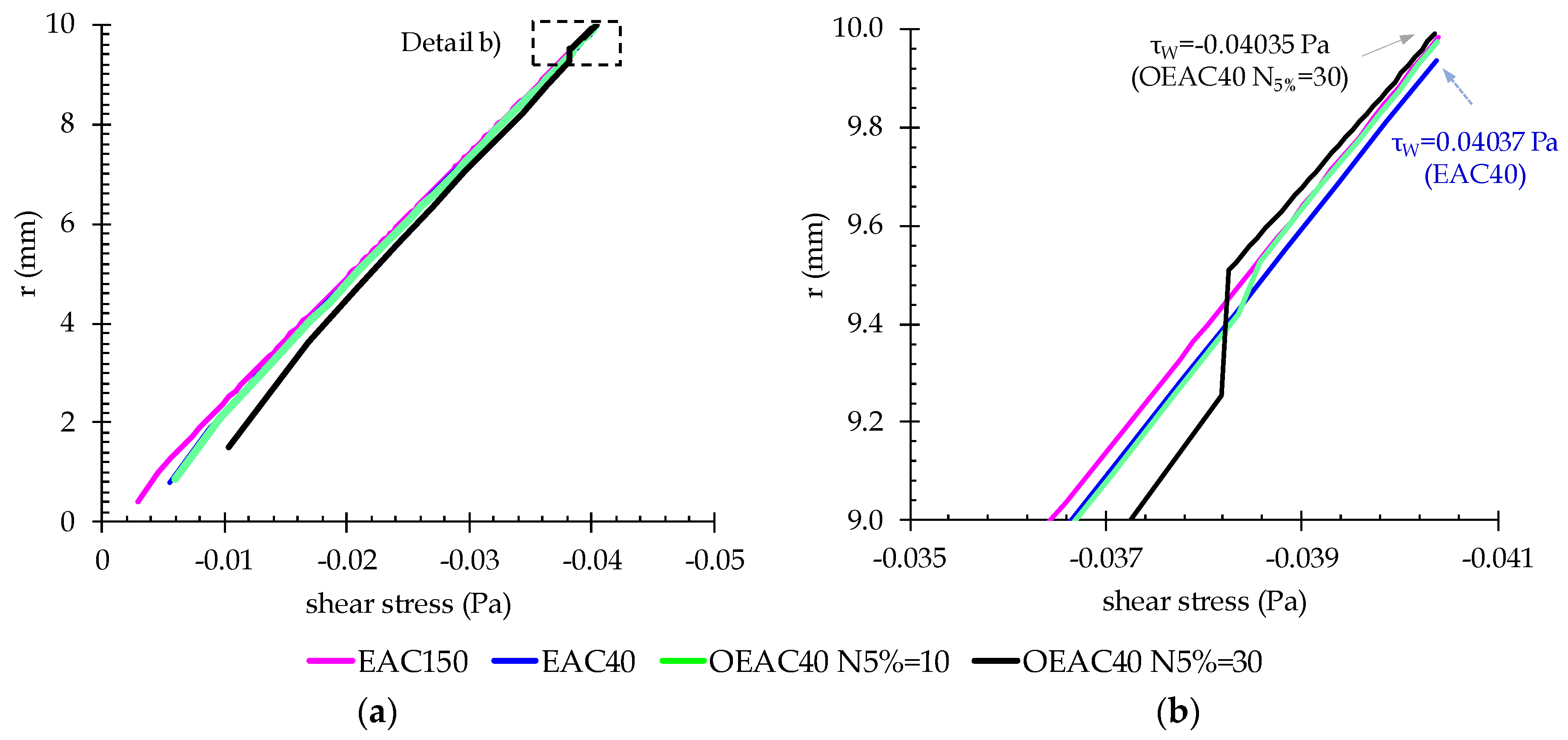
All meshes show similar wall shear stress values close to the pipe wall (see r = 10 mm in Figure 11b). Nevertheless, the highest resolution OEAC meshes tend to have higher shear stress values in the pipe core (see r < 2 mm in Figure 11a). Increasing the distance between grid points, Δ r , towards the pipe axis implies a higher numerical error in the pipe core. Additionally, the OEAC meshes have a discontinuity between the high and the low-resolution regions, this discontinuity being more pronounced for higher values of NHR (Figure 11b; see black and green curves for r = 9.5 mm). This discontinuity occurs in the transition between the two regions of the OEAC meshes (i.e., at r= 9.5 mm), being more noticeable for the OEAC40 N5% = 30 mesh.
The OEAC meshes with high NHR values allow a considerable improvement in the wall shear stress simulation results without increasing 
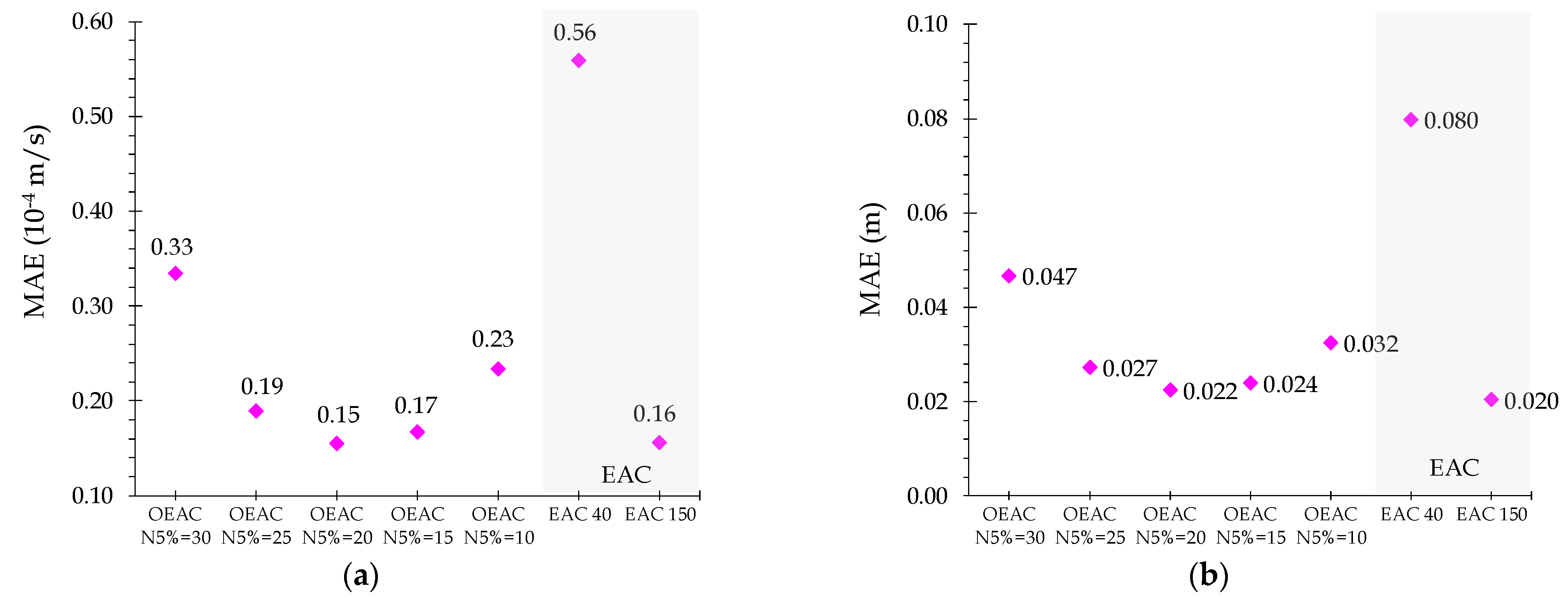
NC; however, a balance with higher steady-state error must be accomplished. The MAE of the mean velocity simulation is calculated in the first wave period (t/T < 1) using Zielke’s model as benchmark, as depicted in Figure 12a. The EAC meshes (EAC40 and EAC150) and OEAC meshes with NC = 40, and varying the NHR values from 30 to 10, are considered. OEAC40 N5% = 20 has the lowest error (MAE = 0.15), close to that of the standard EAC150 (MAE = 0.16) and five times lower than that for the standard EAC40 mesh (with the same number of cylinders). Increasing the number of cylinders in the wall region (NHR from 20 to 30) increases the MAE value because a higher wall shear stress accuracy does not compensate for a lower steady velocity profile accuracy; decreasing the number of cylinders in the wall region also increases the error for the opposite reason. The piezometric-head results lead to the same conclusions (Figure 12b).

5. Numerical Results for the Calibrated Valve Closure

5.1. Introduction

This section presents the analysis of the Q2D model results for a non-instantaneous fast valve maneuver. This maneuver has a S-shape and resulted from the calibration of the 1D and Q2D models with the collected data (see Figure 4a). In this analysis, the NHR/NC = 0.5 ratio is considered, as it presented the best results for an instantaneous valve closure. First, results obtained with traditional radial meshes (i.e., EAC, ETC and GS) are compared and discussed for both steady and unsteady flow conditions. Second, the Q2D results with an OEAC20 mesh are compared with the experimental data and with results from 1D models.

5.2. Comparison with Traditional Meshes’ Results

5.2.1. Steady-State Mesh Assessment

The steady-state mean velocity relative error is assessed for the four analyzed mesh geometries (ETC, EAC, OEAC and GS), according to the total number of cylinders (NC), and presented in Figure 13. The relative error is given by ( U 2 D U 1 D ) / U 1 D in which U 1 D is the input mean velocity and U 2 D is the Q2D model steady-state mean velocity (i.e., after the convergence process).
These results show that the error decreases exponentially with the NC increase. The equal thickness cylinders mesh (ETC) has the best performance. The ETC mesh error drops 25 times with the Δ r reduction to 1/5 (increasing NC from 20 to 100), as expected by the finite difference scheme truncation error, O( Δ r 2 ); see Equation (10). The cylinders have a uniform thickness along the pipe radius, and there is no error associated with the grid non-uniformity.
The non-uniform grids (GS, EAC and OEAC) show a lower error decrease with the NC increase, because the cylinder thickness reduces faster in the wall area than in the pipe core. The OEAC meshes give overall worse results. Only with NC = 60 does this geometry present a higher accuracy than the ETC20 (i.e., with three times the NC value and computer effort). The equal area cylinder mesh (EAC) presents better results than those of the OEAC meshes. The GS mesh does not show the same accuracy improvement with NC increase; for NC = 20, this mesh is close to the best results (ETC20); on the contrary, for NC = 100, it tends to the mesh with the worst results (OEAC100). With the NC increase, the GS geometry focuses its refinement on the wall area, where the axial velocity has lower values. The mesh refinement in the wall area explains the GS slower error reduction with NC and the lower overall performance of OEAC.

5.2.2. Unsteady-State Mesh Assessment

The simulations are carried out for the analyzed four mesh geometries (ETC, EAC, OEAC and GS) and for a 10-wave period. A high-resolution mesh with NC = 300 is considered for benchmark comparison. The number of cylinders for each geometry varies from 20 to 100 (NC = 20, 40, 60, 80 and 100). Figure 14 shows the piezometric head results for the different meshes, plotting only results with significant differences from those of the benchmark mesh.
The OEAC mesh results approach those of the reference mesh, with only 20 cylinders, OEAC20 (Figure 14a). The GS mesh doubles the previous NC value (GS40) to ensure the same global accuracy (Figure 14b). The EAC mesh requires 80 cylinders (i.e., four times the OEAC effort) to achieve the same accuracy (Figure 14c). Only the ETC grid with the maximum number of 100 cylinders (ETC100) and five times the OEAC20 mesh computational effort can ensure the same simulation accuracy (Figure 14d). The wave damping is correctly calculated by most meshes, except for non-OEAC meshes with the lowest NC.
The wall shear stress and piezometric head mean that absolute error, MAE, is calculated at the pipe midsection for the previous four meshes (Figure 15) and for the complete simulation (0 ≤ t/T ≤ 10). The quasi-steady and Trikha [9] 1D model results are also presented, as these represent low computation time solutions. The OEAC grids show an exceptional energy dissipation accuracy for low NC values (NC ≤ 60). Compared with the second-best results (EAC20, GS40 and GS60), this mesh allows an overall error reduction of 86%, 88% and 66% for NC = 20, 40 and 60, respectively. Traditional meshes with a low number of cylinders are not capable of correctly describing the 𝜏 wall peak and its subsequent exponential decay. For higher Nc values (NC ≥ 80), the GS meshes have higher accuracy than the OEAC meshes. EAC and ETC meshes have the worst results: for instance, the OEAC20 has a similar MAE value to the EAC100 and is three times smaller than ETC100, both with five times the new mesh computer effort. The quasi-steady 1D model results are incompatible with an accurate energy dissipation and with double the worst Q2D mesh error (i.e., ETC20). Trikha’s 1D results are comparable with those of low resolution meshes but do not match the best Q2D model’s results.
The OEAC mesh has demonstrated itself to be the best radial geometry in order to calculate unsteady energy dissipation with fewer cylinders; however, these meshes have the highest steady-state error due to the low mesh resolution in the pipe core (Figure 13). The piezometric head MAE calculation (Figure 15b) accounts for both the steady and unsteady simulation accuracy. The piezometric head and wall shear stress MAE results shows a similar behavior. This similarity is due to the minor importance of the steady velocity profile error concerning overall unsteady energy dissipation and OEAC mesh improvement.

5.3. Comparison with Experimental Data

Experimental data are compared with the results from the Q2D model with the OEAC20 mesh (OEAC20 N5% = 10). The quasi-steady and Trihka’s 1D models are also included, for comparison purposes. The analysis excludes Zielke’s 1D model, as it produces similar results to those obtained by the Q2D model, requiring higher computation time. All model simulations consider the calibrated valve closure presented in Figure 4a.
Figure 16a shows the results for the first wave period (0 ≤ t/T ≤ 1). All models present comparable results. This similarity reinforces the idea that the simplest models (quasi-steady and Trikha’s 1D models) are applicable for a first pressure surge simulation or maximum pressure calculation because of the low energy dissipation observed during this short period.
The results are considerably different for a 10-wave periods analysis (Figure 16a,c). The quasi-steady 1D model is not capable of describing the pressure wave attenuation, nor the wave round shape over time, and this model underestimates the pressure damping by 75% at t/T = 10. The Trikha’s model ensures the correct wave damping but not the correct wave shape, with a rectangular shaped pressure front wave, due to this model’s inability to correctly compute the high energy dissipation period immediately after each pressure surge (Figure 16c,d). The previous conclusion, regarding the practical adequacy of 1D models for the estimation of transient pressures in the first pressure wave period, is not valid for longer time periods.
The Q2D model simulation using the optimized mesh and the lowest NC value (OEAC20) ensures both the wave attenuation (compare the Q2D model and the test data for the middle point of each wave peak) and the front wave shape (see Figure 16c,d). However, the Q2D model cannot correctly describe the symmetric wave shape observed in the experimental data.

6. Complete Versus Simplified Q2D Models

Results presented in previous sections refer to the complete Q2D model from Vardy and Hwang (1981) [6], with Zhao and Ghidaoui’s implementation [24]. The simplified Q2D model neglects the lateral mass transfer and allows a computation effort reduction of 30% and 40% with θ1 = 0.5 and θ1 = 1.0, respectively. The accuracy of the three models—complete Q2D, simplified Q2D (θ1 = 0.5) and simplified Q2D (θ1 = 1)—is assessed herein for the instantaneous and for the calibrated valve maneuvers.

6.1. Instantaneous Valve Manoeuvre

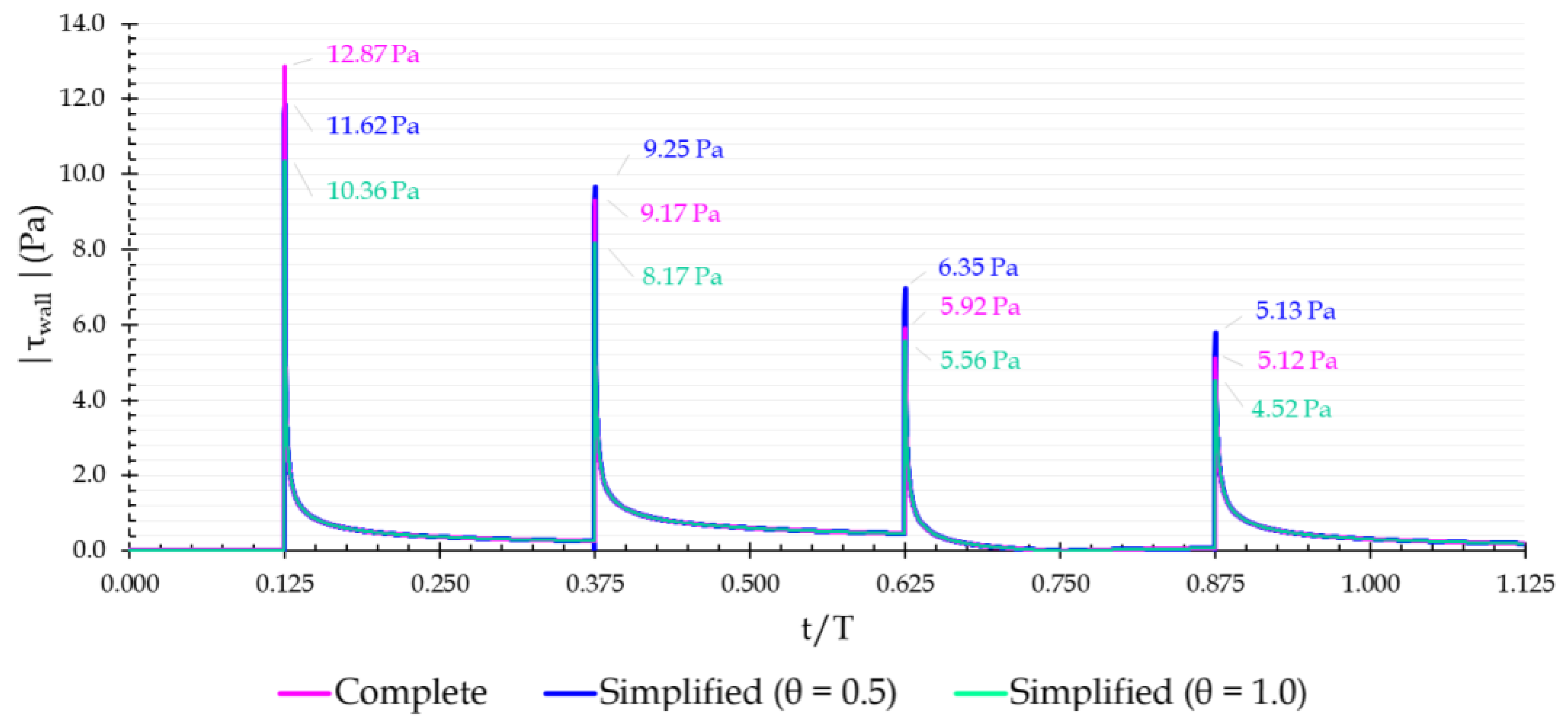
The wall shear stress results are analysed for NC values from 20 to 100 and compared with the Zielke’s analytical solution for ∆x = 0.01m. For NC = 100, a slight difference is registered between the three models during the high velocity-gradient immediately after the pressure surge and fades shortly after (Figure 17). The complete model has the best accuracy, and the simplified model with θ1 = 1.0 the worst. Nevertheless, for the lowest NC meshes (NC = 60 and NC = 80), the differences between the three models are hardly observed because the period immediately after the pressure surge is not described so accurately.
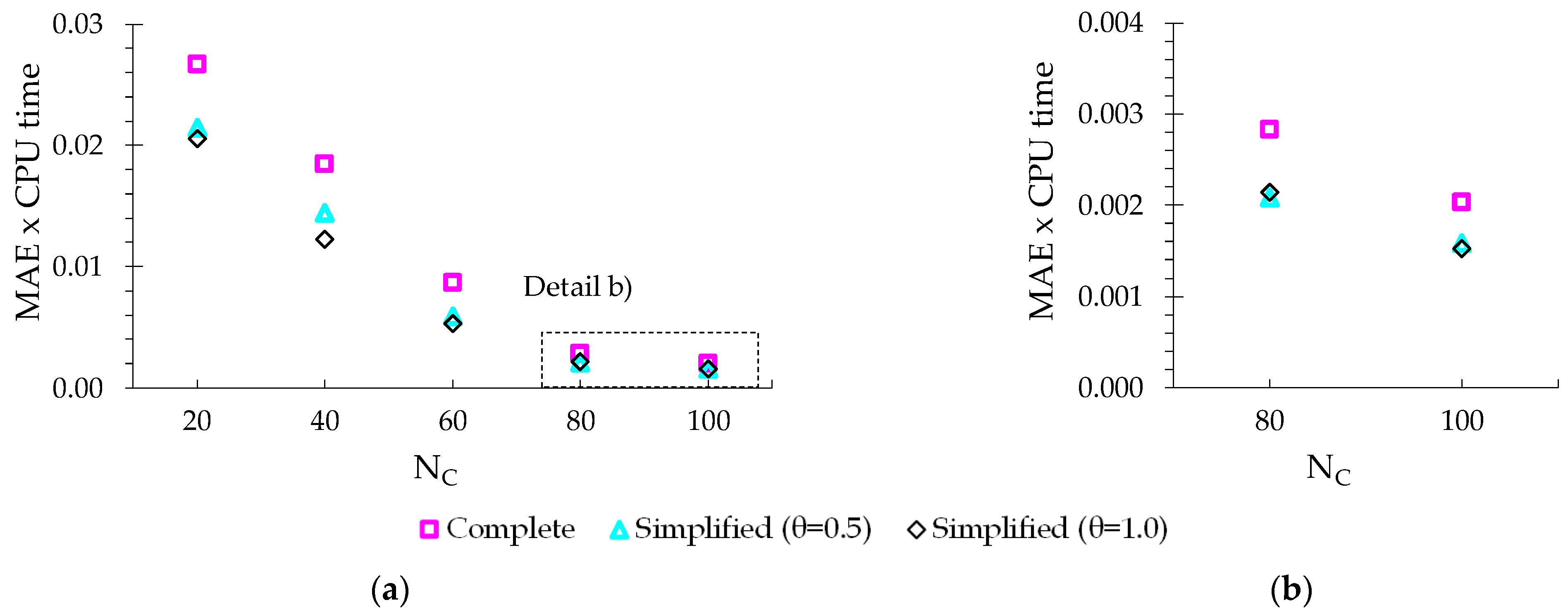
Figure 18 shows the product between the accuracy (described by MAE) and the CPU time for the different NC values. The rationale is to combine these two aspects in a single parameter for best selection of the numerical model. The MAE value exponentially decreases with NC. Increasing the NC value ensures a better simulation accuracy independently of the numerical model selected. Increasing the model complexity is not justifiable for meshes with low NC, and the simplified model with θ1 = 1.0 is the best option. For higher NC values the simplified model with θ1 = 0.5 compensates for the additional computation time. The complete model is only recommended for a detailed evaluation in the period immediately after the pressure surge.

6.2. Calibrated Valve Manoeuvre

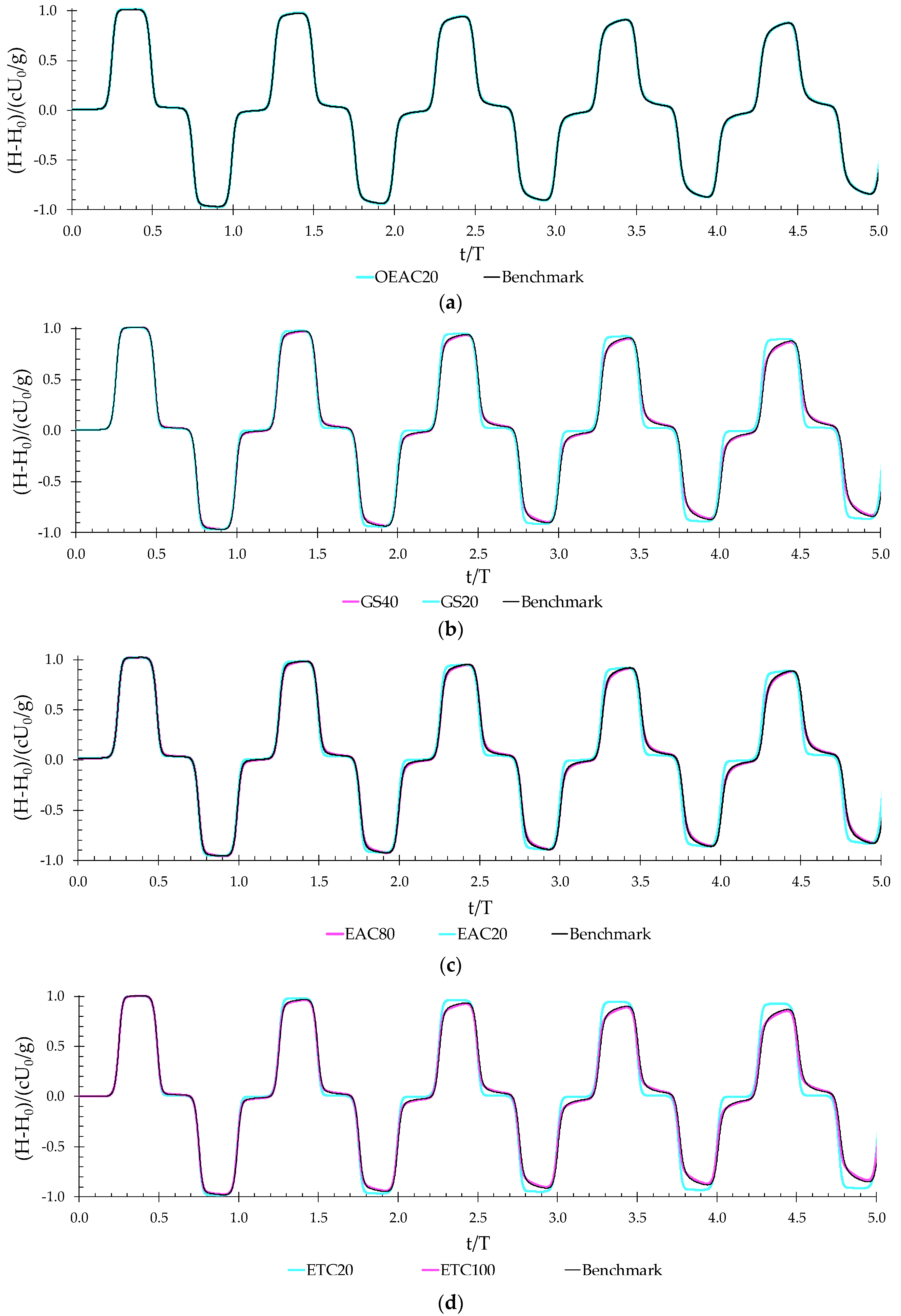
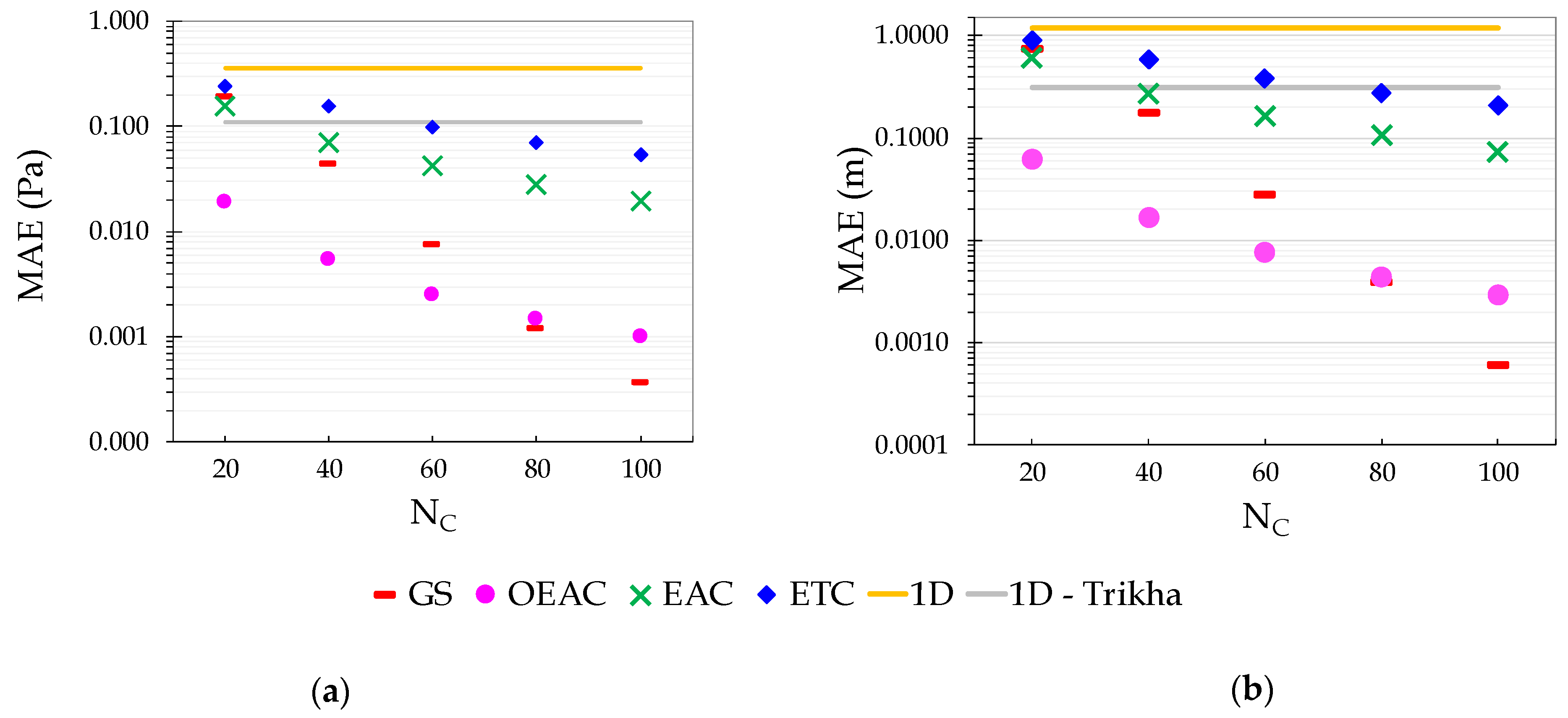
The calibrated valve closure (
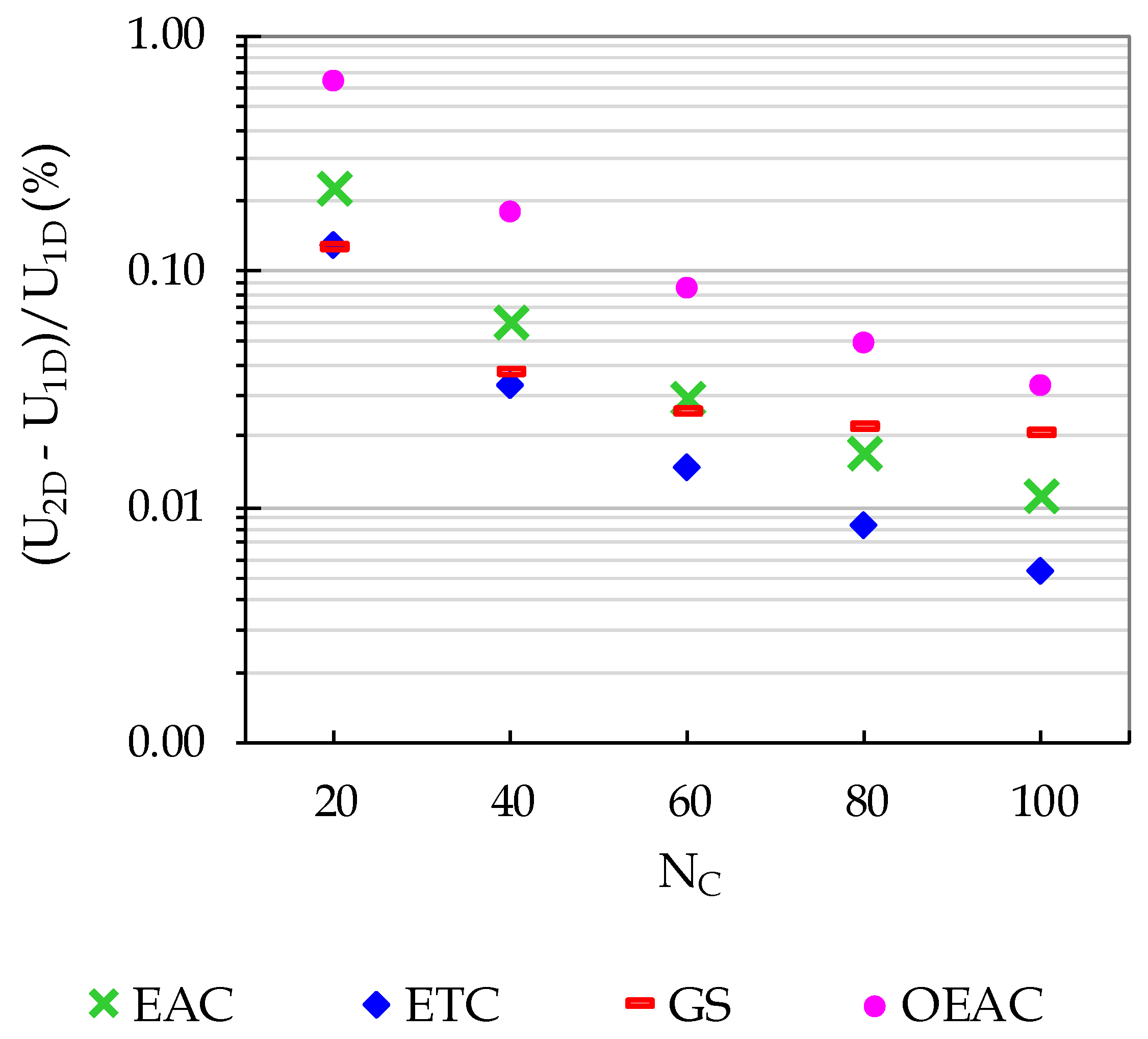
Figure 4) is used to analyze the accuracy of the three numerical models results for the traditional mesh geometries (GS, EAC and ETC) and the new optimized mesh (OEAC). For the sake of simplicity, only the NC = 100 meshes are considered, since the results for lower NC values were negligible for instantaneous valve closure.
A slower valve closure maneuver reduces the wall shear stress peak and, consequently, approximates the results for the three traditional mesh geometry models, compared to the instantaneous valve closure. Additionally, the EAC and ETC meshes show a low accuracy and the simulation results are independent of the selected Q2D model, thus, the fastest numerical scheme should be considered (simplified model with θ1 = 0.5). On the contrary, the results of the high-resolution grids (OEAC and GS) are influenced by the model, and the conclusions are similar to those obtained for the instantaneous valve maneuver.

7. Conclusions

An optimized equal area cylinder (OEAC) radial mesh is proposed to ensure the Q2D model accuracy without increasing the computation effort. The new mesh, with 40 cylinders, is defined by a high-resolution grid near the pipe wall and a lower-resolution grid in the pipe core. For an instantaneous valve closure, this mesh reduced the calculation time by four times with similar simulation error, compared to the standard equal area cylinder (EAC) mesh.
The results of the new mesh are compared with those obtained for the traditional mesh geometries (GS, ETC and EAC) for a calibrated S-shape valve closure. Compared to the geometric sequence (GS) mesh, the new geometry achieved a significant improvement in accuracy for meshes with fewer cylinders (NC ≤ 60). The other two radial meshes (ETC and EAC) do not provide the same accuracy. The new mesh correctly describes the experimental data with only 20 cylinders, which is not achieved by the fastest 1D models.
The simplified Q2D model (i.e., neglecting the lateral velocity) reduces the computational effort without significant loss of accuracy for low resolution meshes in the wall region. If a higher accuracy simulation is required, it is recommended to increase the number of cylinders instead of using the complete Q2D model.
The new two-region mesh has been applied herein to laminar flows, for which there is an exact analytical solution for unsteady friction (Zielke’s formulation) that is used as a benchmark solution for comparison. In future works, the same approach can be applied to turbulent flows by including an adequate turbulent model in the fundamental equations, and the results obtained can be analyzed and compared with experimental data. Additionally, future research could explore the possibility of using a dynamic-mesh, reconfigured during the transient event according to the axial velocity gradient, in order to reduce the computation effort, but maintaining a high accuracy; this will imply the development of a new specific numerical scheme, adequate for non-uniform meshes, to avoid the loss of accuracy due to high grid space variations.

Author Contributions

Conceptualization, P.L.F. and D.I.C.C.; methodology, P.L.F. and D.I.C.C.; software, P.L.F.; validation, P.L.F.; formal analysis, P.L.F.; investigation, P.L.F. and D.I.C.C.; resources, P.L.F. and D.I.C.C.; data curation, D.I.C.C.; writing—original draft preparation, P.L.F.; writing—review and editing, P.L.F. and D.I.C.C.; visualization, P.L.F.; supervision, D.I.C.C.; project administration, D.I.C.C.; funding acquisition, D.I.C.C. All authors have read and agreed to the published version of the manuscript.

Funding

The authors would like to thank the Fundação para a Ciência e Tecnologia (FCT) through funding UIDB/04625/2020 from the research unit CERIS.

Data Availability Statement

The data presented in this study are available upon request from the corresponding author.

Acknowledgments

The authors would like to acknowledge João Paulo Ferreira for assisting the data collection in the experimental facility and for providing additional data.

Conflicts of Interest

The authors declare no conflict of interest.

Nomenclature

Aj, Bj, Cj, Djquasi-2D model coefficients (-)
CRgeometric sequence common ratio (-)
cpressure wave speed (m/s)
Dpipe inner diameter (m)
gacceleration due to gravity (m/s2)
Hpiezometric head (m)
Lpipe length (m)
NCtotal number of cylinders of the radial mesh (-)
NHRtotal number of cylinders in the high-resolution area (OEAC meshes)
NXnumber of axial mesh points in the pipe direction (-)
Qflow-rate or discharge (m3/s)
Rpipe inner radius (m)
ReReynolds number, Re = UD/ν (-)
rdistance from the axis in the radial direction (m)
r j external radius of the jth cylinder measured from the pipe axis (m)
r ¯ j center radius of the jth cylinder measured from the pipe axis (m)
Tpressure wave period, T = 4L/c (s)
ttime (s)
Umean velocity of the fluid in the pipe cross-section (m/s)
uaxial velocity (m/s)
υ radial velocity (m/s)
xdistance along the pipe (m)
tnumerical time step (s)
xnumerical spatial step (m)
rj wall   thickness   of   the   j th   cylinder   ( Δ r j = r j r j 1 )
εpipe wall roughness (m)
θ 1 ,   θ 1 weighting   coefficient   ( θ 1 + θ 2 = 1 )
νkinematic viscosity of liquid (m2/s)
𝜚liquid density (kg/m3)
𝜏wall shear stress (Pa)

Abbreviations

CFDComputation fluid dynamics
CFLCourant-Friedrich-Lewy
EACEqual area cylinder mesh
ETCEqual thickness cylinder mesh
GSGeometric sequence cylinder mesh
MAEMean absolute error
MOCMethod of Characteristics
Q2DQuasi-2D model

References

  1. Leishear, R.A. Fluid Mechanics, Water Hammer, Dynamic Stresses, and Piping Design; ASME: New York, NY, USA, 2012. [Google Scholar]
  2. Chaudhry, M.H. Applied Hydraulic Transients, 3rd ed.; Springer: Berlin/Heidelberg, Germany, 2014. [Google Scholar]
  3. Wylie, E.B.; Streeter, V.L. Fluid Transients in Systems; Prentice Hall: Hoboken, NJ, USA, 1993. [Google Scholar]
  4. Almeida, A.B.; Koelle, E. Fluid Transients in Pipe Networks; Elsevier Applied Science: New York, NY, USA, 1992. [Google Scholar]
  5. Zielke, W. Frequency-dependent friction in transient pipe flow. J. Basic Eng. 1968, 90, 109–115. [Google Scholar] [CrossRef]
  6. Vardy, A.E.; Hwang, K.-L. A characteristic model of transient friction in pipes. J. Hydraul. Res. 1991, 29, 669–684. [Google Scholar] [CrossRef]
  7. Shuy, E.B. Approximate wall shear equation for unsteady laminar pipe flows. J. Hydraul. Res. 2010, 33, 457–469. [Google Scholar] [CrossRef]
  8. Brunone, B.; Ferrante, M.; Cacciamani, M. Decay of Pressure and Energy Dissipation in Laminar Transient Flow. J. Fluids Eng. 2004, 126, 928–934. [Google Scholar] [CrossRef]
  9. Trikha, A.K. An efficient method for simulating frequency dependent friction in transient liquid flow. J. Fluids Eng. 1975, 97, 97–105. [Google Scholar] [CrossRef]
  10. He, S.; Ariyaratne, C.; Vardy, A.E. Wall shear stress in accelerating turbulent pipe flow. J. Fluid Mech. 2011, 685, 440–460. [Google Scholar] [CrossRef]
  11. Pothof, I. A turbulent approach to unsteady friction. J. Hydraul. Res. 2010, 46, 679–690. [Google Scholar] [CrossRef]
  12. Vardy, A.E.; Brown, J.M.B. Approximation of Turbulent Wall Shear Stresses in Highly Transient Pipe Flows. J. Hydraul. Eng. 2007, 133, 1219–1228. [Google Scholar] [CrossRef]
  13. Vardy, A.E.; Brown, J.M.B. Transient, turbulent, smooth pipe friction. J. Hydraul. Res. 1995, 33, 435–456. [Google Scholar] [CrossRef]
  14. Vardy, A.E.; Brown, J.M.B. Transient Turbulent Friction in Smooth Pipe Flows. J. Sound Vib. 2003, 259, 1011–1036. [Google Scholar] [CrossRef]
  15. Vardy, A.E.; Hwang, K.-L. A weighting function model of transient turbulent pipe friction. J. Hydraul. Res. 1993, 31, 533–548. [Google Scholar] [CrossRef]
  16. Vitkovsky, J.P.; Lambert, M.F.; Simpson, A.R. Advances in unsteady friction modelling in transient pipe flow. In Proceedings of the 8th International Conference on Pressure Surges, The Hague, The Netherlands, 12–14 April 2000; Pub. BHR Group Ltd.: The Hague, The Netherlands, 2000; pp. 471–498. [Google Scholar]
  17. Ramos, H.M.; Covas, D.; Loureiro, D.; Borga, A. Surge damping analysis in pipe systems: Modelling and experiments. J. Hydraul. Res. 2004, 42, 413–425. [Google Scholar] [CrossRef]
  18. Brunone, B.; Karney, B.W.; Mecarelli, M.; Ferrante, M. Velocity Profiles and Unsteady Pipe Friction in Transient Flow. J. Water Resour. Plan. Manag. 2000, 126, 236–244. [Google Scholar] [CrossRef] [Green Version]
  19. Vardy, A.E.; Brown, J.M.B. On turbulent, unsteady, smooth-pipe friction. In Proceedings of the 7th International Conference on Pressure Surges and Fluid Transients in Pipelines and Open Channels, Harrogate, UK, 16–18 April 1996; Pub. BHR Group Ltd.: Harrogate, UK, 1996; pp. 289–311. [Google Scholar]
  20. Vardy, A.; Brown, J. Efficient Approximation of Unsteady Friction Weighting Functions. J. Hydraul. Eng. 2004, 130, 1097–1107. [Google Scholar] [CrossRef]
  21. Urbanowicz, K.; Zarzycki, Z. Improved Lumping Friction Model for Liquid Pipe Flow. J. Theor. Appl. Mech. 2015, 53, 295–305. [Google Scholar] [CrossRef] [Green Version]
  22. Urbanowicz, K. Analytical expressions for effective weighting functions used during simulations of water hammer. J. Theor. Appl. Mech. 2017, 55, 1029–1040. [Google Scholar] [CrossRef] [Green Version]
  23. Bratland, O. Frequency-dependent friction and radial kinetic energy variation in transient pipe flow. In Proceedings of the 5th International Conference on Pressure Surges, Hannover, Germany, 22–24 September 1986; BHRA, The Fluid Engineering Centre: Hannover, Germany; pp. 95–101. [Google Scholar]
  24. Zhao, M.; Ghidaoui, M. Efficient quasi-two-dimensional model for water hammer problems. J. Hydraul. Eng. 2003, 129, 1007–1013. [Google Scholar] [CrossRef]
  25. Pezzinga, G. Quasi-2D model for unsteady flow in pipe networks. J. Hydraul. Eng. 1999, 125, 676–685. [Google Scholar] [CrossRef]
  26. Korbar, R.V. Efficient solution method for quasi two-dimensional model of water hammer. J. Hydraul. Res. 2014, 52, 575–579. [Google Scholar] [CrossRef]
  27. Korbar, R.V. Truncated method of characteristics for quasi-two dimensional water hammer model. J. Hydraul. Eng. 2014, 140, 04014013. [Google Scholar] [CrossRef]
  28. Alizadeh Fard, M.; Baruah, A.; Barkdoll, B.D. CFD modeling of stagnation reduction in drinking water storage tanks through internal piping. Urban Water J. 2021, 18, 608–616. [Google Scholar] [CrossRef]
  29. Martins, N.M.C.; Delgado, J.N.; Ramos, H.M.; Covas, D.I.C. Maximum transient pressures in a rapidly filling pipeline with entrapped air using a CFD model. J. Hydraul. Res. 2017, 55, 506–519. [Google Scholar] [CrossRef]
  30. Martins, N.M.C.; Soares, A.K.; Ramos, H.M.; Covas, D.I.C. CFD modeling of transient flow in pressurized pipes. Comput. Fluids 2016, 126, 129–140. [Google Scholar] [CrossRef]
  31. Simao, M.; Mora-Rodriguez, J.; Ramos, H.M. Computational dynamic models and experiments in the fluid-structure interaction of pipe systems. Can. J. Civil. Eng. 2016, 43, 60–72. [Google Scholar] [CrossRef]
  32. Gidaspow, D.; Li, F.; Huang, J. A CFD simulator for multiphase flow in reservoirs and pipes. Powder Technol. 2013, 242, 2–12. [Google Scholar] [CrossRef]
  33. Martins, N.M.C.; Carriço, N.J.G.; Ramos, H.M.; Covas, D.I.C. Velocity-distribution in pressurized pipe flow using CFD: Accuracy and mesh analysis. Comput. Fluids 2014, 105, 218–230. [Google Scholar] [CrossRef]
  34. Hirsch, C. Numerical Computation of Internal & External Flows, 2nd ed.; Elsevier: Oxford, UK, 2007. [Google Scholar]
  35. Ferziger, J.H.; Perić, M. Computational Methods for Fluid Dynamics; Springer: Berlin/Heidelberg, Germany, 1996. [Google Scholar]
  36. Ferreira, J.P.; Martins, N.M.C.; Covas, D.I.C. Ball Valve Behavior under Steady and Unsteady Conditions. J. Hydraul. Eng. 2018, 144, 04018005. [Google Scholar] [CrossRef]
  37. Ferreira, J.P.; Buttarazzi, N.; Ferras, D.; Covas, D.I.C. Effect of an entrapped air pocket on hydraulic transients in pressurized pipes. J. Hydraul. Res. 2021, 59, 1018–1030. [Google Scholar] [CrossRef]
  38. Ferras, D.; Manso, P.A.; Schleiss, A.J.; Covas, D.I.C. Fluid-structure interaction in straight pipelines with different anchoring conditions. J. Sound Vib. 2017, 394, 348–365. [Google Scholar] [CrossRef]
  39. Ferràs, D.; Manso, P.A.; Schleiss, A.J.; Covas, D.I.C. Experimental distinction of damping mechanisms during hydraulic transients in pipe flow. J. Fluids Struct. 2016, 66, 424–446. [Google Scholar] [CrossRef]
  40. Martins, N.M.C.; Brunone, B.; Meniconi, S.; Ramos, H.M.; Covas, D.I.C. Efficient Computational Fluid Dynamics Model for Transient Laminar Flow Modeling: Pressure Wave Propagation and Velocity Profile Changes. J. Fluids Eng. 2018, 140, 011102. [Google Scholar] [CrossRef]
  41. Martins, N.M.C.; Brunone, B.; Meniconi, S.; Ramos, H.M.; Covas, D.I.C. CFD and 1D Approaches for the Unsteady Friction Analysis of Low Reynolds Number Turbulent Flows. J. Hydraul. Eng. 2017, 143, 04017050. [Google Scholar] [CrossRef]
Figure 1. Radial grid system for numerical solution with Q2D model.
Water 15 01402 g001
Figure 2. Radial meshes with different geometries for NC = 40: (a) GS5%40; (b) EAC40; and (c) ETC40.
Water 15 01402 g002
Figure 3. Experimental test facility: (a) upstream anchored copper pipe; (b) downstream pipe end; and (c) pneumatically actuated ball valve.
Water 15 01402 g003
Figure 4. Calibrated valve maneuver for laminar flow: (a) Q2D model flow rate variation; (b) experimental and Q2D model piezometric head variation.
Water 15 01402 g004
Figure 5. Q2D simulations for EAC meshes with increasing NC using Zielke’s 1D model as benchmark: (a) wall shear stress; (b) piezometric-head; (c,d) details of the piezometric-head.
Water 15 01402 g005
Figure 6. Axial velocity for four instances equally spaced in time during the first pressure wave: (a) complete pipe radius, 0 ≤ r (mm) ≤ 10; (b) close to the pipe wall, 8 ≤ r (mm) ≤ 10.
Water 15 01402 g006
Figure 7. Radial mesh for the OEAC40 N5% = 20.
Water 15 01402 g007
Figure 8. Wall shear stress obtained for OEAC meshes and for the Zielke’s 1D model: (a) OEAC40 N5% = 30; (b) OEAC40 N5% = 20; (c) OEAC40 N5% = 10.
Water 15 01402 g008
Figure 9. Mean absolute error (MAE) for the wall shear stress for different meshes.
Water 15 01402 g009
Figure 10. Steady-state velocity profile error for standard and optimized meshes.
Water 15 01402 g010
Figure 11. Shear stress profile for EAC40, EAC150, OEAC40 N5% = 10 and OEAC40 N5% = 30: (a) 0 ≤ r ≤ 10 mm; and (b) 9.0 ≤ r ≤ 10 mm.
Water 15 01402 g011
Figure 12. MAE for EAC and varying the NHR value in OEAC meshes: (a) wall shear stress; (b) piezometric head.
Water 15 01402 g012
Figure 13. Steady-state mean velocity error according to the total number of cylinders (log scale).
Water 15 01402 g013
Figure 14. Piezometric head time history for the S-shape valve closure: (a) OEAC, (b) GS, (c) EAC, and (d) ETC.
Water 15 01402 g014
Figure 15. MAE according to Nc and radial geometry. (a) Wall shear stress, (b) piezometric head.
Water 15 01402 g015
Figure 16. Piezometric head time history at conduit midsection, comparing experimental data, quasi-2D and 1D models: (a) 0.0 ≤ t/T ≤ 10.0; (b) 0.0 ≤ t/T ≤ 1.0; (c) 9.0 ≤ t/T ≤ 10.0.
Water 15 01402 g016
Figure 17. Wall shear stress simulation at pipe midsection for NC = 100. 0.0 ≤ t/T ≤ 1.25.
Water 15 01402 g017
Figure 18. MAE and CPU time product calculation for the three numerical schemes using 1D Zielke model as benchmark: (a) for 20 ≤ NC ≤ 100; and (b) detail for NC = 80 and 100.
Water 15 01402 g018
Disclaimer/Publisher’s Note: The statements, opinions and data contained in all publications are solely those of the individual author(s) and contributor(s) and not of MDPI and/or the editor(s). MDPI and/or the editor(s) disclaim responsibility for any injury to people or property resulting from any ideas, methods, instructions or products referred to in the content.

