Shoreline Temporal Variability Inferred from Satellite Images at Mar del Plata, Argentina

Abstract

Sandy beaches are fragile and dynamic coastal areas exposed to numerous environmental forcings. Systematic long-term data acquisition programs and exhaustive data series analyses are fundamental for a comprehensive understanding of the coastal processes. The software CoastSat was implemented to detect the shoreline position at beaches located to the south of Mar del Plata city (Buenos Aires Province, Argentina), by means of satellite images (period: 1986–2020). Tides in this area are mixed semidiurnal with a mean range of 1.74 m. The most frequent waves are characterized by significant wave heights from 0.5 to 2 m and periods of around 8 s propagating mainly from SSE. Seasonal and interannual variability and long-term trends of the shoreline position were investigated at Punta Mogotes (PM) bay, Faro Norte (FN) bay, and Ensenada Mogotes (EM). Seasonal cycles were noticed in the beach width variation series. In general, maximum accumulation was observed in summer and maximum erosion in winter. Exceptions were appreciated at southern PM bay (maximum accretion in autumn and maximum erosion in spring) and at FN bay (beach rotation on a seasonal scale). The drivers of seasonal variation are likely seasonal variations in the significant wave height and direction. PM bay showed a strong interannual variability with a clear alternating pattern between the northern and southern sectors of the bay, in an 8 ± 1.2 years period. Long-term trends showed a generalized erosion along 9 of the 12 km of the analyzed coast.

1. Introduction

Sandy beaches are complex environmental systems controlled by a high number of forcings, such as wind, tides, surges, waves, nearshore currents, and human interventions. Therefore, beach morphology is constantly adjusting to changes or variations in these forcings in different temporal scales, i.e., short-term changes, seasonal variability, interannual variability, and long-term trends [1]. Systematic long-term data acquisition programs and exhaustive data series analyses are fundamental for a comprehensive understanding of these coastal processes. For instance, an interannual signal could be misunderstood as a gentle long-term trend when it is detected from a relatively short data series [2]. On the contrary, severe beach erosion produced by coastal storms during the occurrence of extratropical cyclones [3] or extreme seasonal wave conditions, could be wrongly linked to climate variability. Consequently, a systematic and sustained coastal monitoring plan becomes mandatory to elucidate the most convenient strategy for environmental management [4]. Environmental data and an appropriate plan constitute the cornerstone for coastal managers and researchers, mainly due to the enormous attractiveness of coastal areas and their increasing population growth [5]. The impact of climate change on coastal areas has been extensively researched worldwide [6,7,8,9,10]. The significance of taking into account the effects of climate change on coastal erosion and shoreline retreat was emphasized by [10]. Long-term data series have become increasingly important to understand the future effects of climate change [6,7,8]. Nevertheless, coastline monitoring programs are scarce and limited to only a few sites around the world [11,12,13]. In situ measurements provide accurate data but present limitations when covering great spatial extensions and high-frequency surveys, especially for low-income countries. In this sense, the growth in the availability of satellite imagery provides an opportunity to analyze large and high-frequency datasets gathered from public platforms (such as Google Earth Engine) [14], especially where in situ data are scarce or even nonexistent.

The satellite-derived shoreline has been widely used for coastal monitoring, where different image processing approaches [15] have proven to capture shoreline position (e.g., [16,17,18,19,20,21]). The shoreline, defined as the interface between land and water surface, provides an important indicator of beach variability and change, and is the most widely used indicator to quantify erosion–accretion changes in coastal areas [22,23]. Shoreline change analysis from aerial photos and topographic charts was historically used to analyze the long-term shoreline trend by means of low-frequency data and manual identification (e.g., [24,25,26,27,28]). Recently, the possibility of automatically extracting the shoreline position from large datasets of mid-resolution satellite imagery has become a breakthrough, giving the possibility to capture its variability by the mid-frequency temporal data [18,20,29,30,31]. A global dataset has been built to assess the state of world beaches using automatic extraction “https://aqua-monitor.appspot.com/?datasets=shoreline (accessed on 7 December 2022)”, from [29]. Nevertheless, several uncertainties could be derived from shoreline extraction to generate a robust shoreline change analysis [32]. For instance, the selection of a specific index with a threshold could broadly impact the final ability of the technique to capture the shoreline position [32].

Mar del Plata, located in Buenos Aires Province (Figure 1), is the most important Argentinean coastal city. It concentrates a large part of the tourist activity in the country, especially in the summer, when the number of visitors can quadruplicate the stable population of the city [33]. After the construction of the local port, accretional and erosive processes became evident at beaches located southward and northward of the harbor, respectively. For several decades an important sector of the city’s coast has been suffering from chronic erosion. Different types of legal and illegal initiatives have been developed to mitigate the impacts of shoreline retreats [34]. The southern coast of Mar del Plata has been the subject of numerous studies, mainly by means of in situ beach profiles [35,36,37,38]. These studies generally reported erosive processes in some specific locations of this the sector of the coast.

This paper aims to characterize the variability at different temporal scales and the long-term trends of the shoreline position, during the last 35 years, at the southern sandy beaches of Mar del Plata. In Section 2, a brief description of the study area is presented and the methodology is described. A summary of the parameters, the implemented workflow, and the validation of the CoastSat Python toolkit [30] are included. The results of the analysis of the different temporal scales of variability are found in Section 3, and the discussion is given in Section 4. Finally, the conclusions of this work are presented in Section 5.

2. Materials and Methods

2.1. Study Area

The study area spans 12 km of shoreline placed southward of Mar del Plata city, where three different sections of sandy beaches were analyzed: Punta Mogotes bay (PM), Faro Norte bay (FN), and Ensenada Mogotes (EM) (Figure 1). Tides in this area are mixed semidiurnal with a mean range of 1.74 m “http://www.hidro.gov.ar/oceanografia/Tmareas/RE_Mareas.asp (accessed on 23 March 2021)”. The coincidence of large or even moderate high tides and large meteorologically induced surges has historically caused catastrophic floods and destruction in many coastal areas of the coast [39]. Locally called “sudestada”, storm surge events are frequent, mainly in the winter season, lasting around 26–28 h [40]. The mean and maximum breaking waves are 0.9 m and 4 m, respectively. The main wave propagation direction is from ESE, but they commonly propagate between ENE and SE [41,42]. Wave parameters from Copernicus Marine Environment Monitoring Center (CMEMS) global multi-year product GLOBAL_REANALYSIS_WAV_001_032, also known as Waverys [43], were used to characterize the wave climate seasonality in the study area (Section 3.1). Mean significant wave height (Hs), peak periods (T), and directions with a 3-h time step were analyzed between 1996 and 2020, at the location indicated with a red star in Figure 1b. The beach sediments are composed mainly of quartz sand [36]. The wave climate drives a net northward longshore sediment transport, ranging from 0.3 to 1.0 × 10⁶ m³/y [44]. The longshore drift is largely intercepted by the southern breakwater of the harbor (built-in 1922), producing significant erosive processes northward of the port [45].

PM bay is essentially a 4 km long sandy beach and extends from the southern breakwater of Mar del Plata port to a noticeable outcrop of quartzite rocks (Figure 1). The bay presents NNE-SSO orientation and an asymmetry due to a northward net longshore sediment transport. The Punta Mogotes Complex (CPM), which represents 40% of Mar del Plata’s “shadow units”, attracts a large number of tourists during the summer [46]. A private entity has been extracting sand from the beach for more than 25 years between PM bay and the southern breakwater of the port (Figure 1). FN bay is a 1.4 km long, sandy beach nestled between two outcrops of quartzite rocks (Figure 1). Beach nourishment, with around 1200 tons of sand from crushed quartzite rocks, was carried out at the southern sector of the bay in November 2014 to remediate the erosive processes. It was estimated that around 98% of the overturned sediment was lost during the first year, and the whole amount of filled sand was gone after the second year [37]. The coastline along EM is 5.2 km long and is bounded by an active loess cliff in the southern sector, with a variable height between 15 and 28 m. This cliff extends 25 km southwards, noticing incipient pocket beaches (Figure 1). At the northern sector of EM, the cliff is partially covered by hanging dunes, mostly vegetated and fixed [47]. Wave diffraction and higher breaking waves are noticeable on the sandy salient between FN and EM. The estimated coastal retreat reduced from −3.3 m/year (1985–1988) to −2.5 m/year (1988–1992) [37]. A system of four breakwaters parallel to the coastline, 230 m far from the beach, was emplaced in the southern area of EM to mitigate coastal erosion (Figure 1).

2.2. Shoreline Detection

CoastSat toolkit [30] is an open-source software written in the programming language Python that enables users to obtain a time series of shoreline positions at any coast worldwide, using available satellite imagery from the Google Earth Engine platform. CoastSat was used with the Landsat missions L5 (1986–2012), L7 (1999–2020), L8 (2013–2020), and Sentinel mission S2 (2015–2020). Top-of-atmosphere reflectance images were used with 30 m resolution and 16-days revisit time from the Landsat missions (Tier 1), and 10 m resolution and 5-days revisit from Sentinel 2 mission (Level-1C). Two polygons with areas of 6.2 km² in PM bay and 12.5 km² in FN and EM sites were set for the period 1986–2020. A pixel cloud cover threshold was set to 20% after a sensitivity test at PM, discarding images with more than 20% of the pixels masked by cloudiness in the process. The toolkit also enhances the spatial resolution of the images by the data fusion method known as “pansharpening” [17] and by bilinear interpolation for Landsat images, reaching half of its original pixel size.

The shoreline is detected by means of two main steps: (i) image classification and (ii) subpixel resolution border segmentation [30]. In order to improve the sand–water interface detection, a neural network classifier was trained in the area of interest, using 50 images for each polygon whose pixels were manually labeled in the categories sand, water, foam, vegetation, and building. The “Modified Normalized Difference Water Index” (MNDWI) was used for the detection of water. During processing, in cases where the shoreline cannot be correctly defined, it is possible to discard the images. As an illustrative example of the procedure applied to all polygons, Figure 2 shows the detection of the coastline from the polygon that includes EM and FN using images from all satellite missions. It can be appreciated that the L7 satellite mission has a fault in the Scan Line Corrector sensor [48], producing uniform parallel stripes from 30 m wide in the center of the scene up to 420 m at the edges (Figure 2b). For this reason, intermittent shorelines were acquired with the images from the L7 mission.

Shore-normal transects were defined over the study area to quantify the beach width change. Ten regularly separated transects (300 m apart) were defined at PM (PM1 to PM10, numerated from N to S), and an additional transect on the salient (PM11) (red transects, Figure 1). Three transects were defined at FN: one at each extreme (FN1 and FN3) and another in the center of the bay (FN2) (black transects, Figure 1). Thirteen transects were defined at EM: six regularly spaced (500 m) from EM2 to EM7, one at the headland (EM1) (green transects, Figure 1), and six transects at the breakwaters zone (RO) (blue transects, Figure 1). The origin (zero) of each transect was set at the upper point of the beach. In this way, the coordinate of the inferred coastline position on the transect directly depicts the beach width (BW). The horizontal variation of BW along the transect due to the tide (Δx) was estimated as (Z_REF − Z_TIDE)/s [19], where Z_REF is the tidal datum, Z_TIDE the sea level corresponding to the image time, and s the typical beach slope. The beach slopes used in this work were obtained from in situ beach profiles compiled in [36], corresponding to the characteristic values of different sectors of the study area, and were considered constant in time. Sea level series were measured hourly by the Servicio de Hidrografía Naval (SHN) of Argentina at the Mar del Plata tidal station, located approximately 10 km northwards to the study area. The data series presented some missing data (gaps) throughout the analyzed period (1986–2020); consequently, in these cases, the satellite images were not considered (around 20% of the cases). BW series (between 596 and 768 values) were obtained for each transect after applying the above-explained methodology for the studied period (1986–2020), from a total of 812 shoreline detection in PM polygon and 924 shoreline detections in EM and FN polygon. Data density is higher for recent years (increase in satellite missions) and for the summer months (less cloud cover).

2.3. Beach Width Variation

The Beach Width Variation (BWV, in m) was obtained by subtracting the mean beach width from each BW, for the complete analyzed period. In this way, BWV can be simply seen as an anomaly of BW, where values of BWV lower (greater) than zero indicates that BW is lower (greater) than the mean BW value. Considering the irregular sampling frequency of the satellite data acquisition, the monthly mean BWV was assessed to obtain a regularly time-spaced data series for each transect. To analyze the seasonality of the time series, an additive time series model was used to subtract the 12-month moving average, and the average value for each month was computed over the entire period. Seasonality was assessed by considering the average value of the three months in each season. A space–time semivariogram methodology [49] was implemented to analyze the variability of BWV series at PM Bay. An empirical semivariogram estimates the typical magnitude of the change between two points, considering a temporal lag. It has previously been applied in coastal studies to characterize the spatial variability of beaches (see, for instance, [19,50,51]). BWV long-term trends were calculated using Sen’s slope estimator [52], and its significance (95% confidence) was tested with the Mann–Kendall seasonal trend test for the period 1986–2020.

The methods applied in this work have been widely used in different sites around the world [19]. The performance of the detected shorelines was evaluated by comparing them with in situ beach profiles surveyed in the study area. Beach profiles were measured by means of a level station, with a single cross-shore line measuring every 10 m. The profiles were performed by the by the SHN between 2015 and 2016 at PM and EM, and by the Instituto de Geología de Costas y del Cuaternario (IGCyC) between 2014 and 2015 in FN (Figure 1). The cross-shore satellite transects were selected matching with the in situ beach profiles, and a temporal tolerance of up 15 days was set between the satellite data acquisition and the in situ beach profile measurement. Scatter plots between BW inferred from beach surveys and satellites at PM (period: 2015–2016, satellite missions: S2 and L8), FN (2014–2015, L7 and L8) and EM (2015–2016, L8), and the best linear fits are presented in Figure 3. Correlation coefficients (R²) are greater than 0.8 and root mean square errors (RMSE) range from 10.2 m to 21.7 m.

3. Results

3.1. Seasonal Variability

The rose diagram for Hs and directions for the period (1996–2020) is presented in Figure 4a, along with those corresponding to summer and winter ones (Figure 4b,c, respectively). The most frequent waves are characterized by Hs from 0.5 to 2 m and T of around 8 s, propagating mainly from SSE. In summer, Hs is slightly lower than heights corresponding to the total period, with predominant Hs around 0.5–1.5 m and a dominant propagating direction from ENE (Figure 4b). The highest Hs occurs in winter (1–3 m) with a notably direction from SSE and S (Figure 4c).

BW series are normally distributed (according to the Shapiro–Wilkens test) with mean values ranging from 47 ± 24 m (at RO1) to 334 ± 37 m (at EM1) (period: 1986–2020). Maximum BWV were 81 ± 22 m, 50 ± 15 m, and 143 ± 30 m at PM Bay, FN Bay, and EM, respectively. Seasonal cycles were appreciated in BWV series, with amplitudes (i.e., the difference between the highest and the lowest BWV or BW for a given transect) irregularly distributed in the study area (Figure 5). Amplitudes of about 7 ± 2 m were appreciated from PM1 to PM6, at northern PM Bay (maximum accumulation occurred in summer and maximum erosion in winter). In addition, amplitudes around 8 ± 2 m were observed from PM7 to PM10, at southern PM Bay (maximum accretion occurs in autumn and maximum erosion in spring). The minimum amplitude (2 m) in the seasonal cycle was obtained at PM11. On the other hand, a seasonal cycle was observed at FN1 with an amplitude of around 7 m (highest accumulation in winter and maximum erosion in summer), but the process is reverted at FN3, where the maximum accretion occurred in summer and the maximum erosion in winter, with a BWV amplitude of 12 m (Figure 5). FN2 presented an almost negligible seasonal cycle (3 m amplitude). The highest BWV amplitude was around 30 m at EM1, with a minimum BWV in winter and a maximum in summer. A clear seasonal cycle was found at EM and RO, with maximum accretion in summer and maximum erosion in winter (Figure 5a,c). For illustrative purposes, Figure 5e presents the BWV monthly average for the EM6 transect, where the maximum values are observed in summer and the minimum values in winter.

3.2. Interannual Variability

Significant wave heights and wave directions were analyzed for the periods 1997–2004, 2005–2012, and 2013–2020. The results show that, for the period of 1997–2004, the dominant wave heights ranged from 1.5 to 2.5 m, with waves propagating mainly from the S and SSE. These characteristics are consistent with those found for the entire period analyzed (Figure 4a). During the period 2005–2012, the most common wave heights ranged from 1.0 to 1.5 m, propagating mainly from the SSE. Additionally, the frequency of waves from the SE decreased while the frequency of waves from the ENE and ESE increased. The period 2013–2020 exhibited wave characteristics similar to those of the 1997–2004 period, but with greater wave heights coming from the S.

Interannual variability was appreciated in BWV series at PM Bay. The longest cycles seem to be in the counter phase between BWV series at PM1 and PM10 (Figure 6). The space–time semivariogram showed a mean period of the variability of 8 ± 1.2 years for the transects located at PM Bay, with periods ranging from 6.5 to 9.6 years, and a corresponding BWV amplitude of 17 ± 3.3 m (BWV ranged from 9.6 to 20.2 m). This means that a variation cycle of the shoreline could occur every 7–9 years, with BWV amplitude of around 14–20 m. Complete BWV series (period: 1986–2020) were divided into four subseries that were each 8 years long (1989–1996, 1997–2004, 2005–2012, and 2013–2020). Significant trends were found at almost all transects. A cycle or period (8 years) was appreciated between the occurrence of positive and negative BWV (Figure 6). The greatest positive trend was 5.5 m/year at PM8 (period: 2005–2012), and the greatest negative trend was −6.5 m/year at PM10 (period: 1997–2014). A clear alternating pattern can be observed between the northern and southern sectors of PM Bay, between 2005–2012 and 2013–2020, showing an alternate of trends with opposite signs and similar magnitudes (Figure 7c,d, respectively).

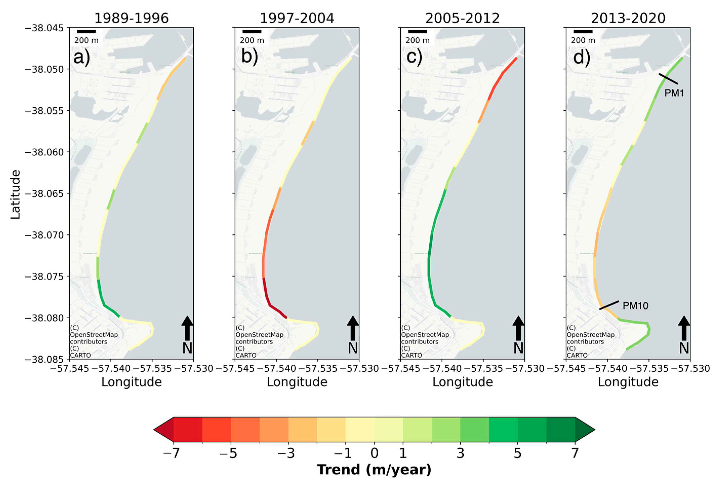
3.3. Long-Term Trends

BWV long term trends (period: 1986–2020) were assessed and, in general, showed a generalized erosion (from −0.2 to −1.9 m/year) in the study area (Figure 8). For instance, negative significant trends (erosion) were detected between PM1 and PM4, which are attenuated southwards from −1.4 to −0.2 m/year, and at PM11 (−0.4 m/year). No significant trends were found at PM5, and from PM8 to PM10. Weak but significant positive trends (around 0.3 m/year) were found at PM6 and PM7. FN1 did not display a significant trend, while FN2 and FN3 showed −0.4 and −0.5 m/year, respectively. In general, significant negative BWV trends were found along the EM coast, but the values were quite spatially irregular. The trends were −1.4 m/year at EM1, not significant at EM2, and increased from EM3 (−0.2 m/year) to EM7 (−1.8 m/year).

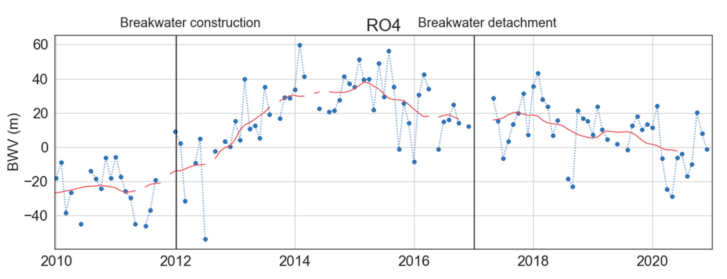
3.4. Anthropic Interventions

Anthropogenic intervention is relatively high in the study area, with the Port of Mar del Plata and several coastal structures found along the beaches located south of the EM (Figure 1). Four breakwaters parallel to the coast were emplaced in this area (Figure 1d). The construction of the breakwater system began in 2011 and finished in 2017. However, the works were interrupted at the end of 2012, with only three breakwaters completed (those furthest south) and without having removed the temporary connecting path to the beach of the one located in transect RO3 (Figure 1) [34]. Work resumed in 2016, with the construction of the fourth breakwater and the removal of the last connecting path in early 2017. These temporary roads worked as little groynes retaining the long-shore sediment transport. During this work, approximately 250,000 m³ of sand were used for nourishment [53]. Unfortunately, there is no record of when the beach nourishment tasks were carried out. The impact of these coastal structures is clearly represented in Figure 9. Monthly (blue dots) and smoothed BWV series (one-year mobile average, red line) represents the beach growth between 2013 and 2015 at RO4, and a very slow and gradual reduction of BWV from 2015 to 2020, from +60 m to around zero. The irregular beach nourishment activity could explain the higher values of BWV observed between 2013 and 2016 in RO4 (Figure 9). Previous to the breakwater emplacement, BWV reached up 40 m below its mean position at RO4.

4. Discussion

A novel and open-source methodology for shoreline extraction was implemented to account for beach variability and long-term processes in an area of great economic and social interest, which has been the focus of numerous coastal studies, mainly based on in situ beach profiles [35,36,37]. The main shortcoming of these studies is the lack of space–time resolution, hindering the overall beach variability representation. The implemented methodology made it possible to study three adjacent sectors of 12 km of sandy beaches located at the southern Mar del Plata Port, between 1986 and 2020. The Google Earth Engine platform allows for the analysis of freely accessible satellite data in the form of top-of-atmosphere reflectance images, through access to and managed storage of big data. Erosive processes were widely documented in the study area [34], but were not described with the relatively high space–time resolution used in this work. In this paper, only around 3 km of the coastal area was found to be stable (no significant long-term trends), and the other 9 km of shoreline showed noticeable erosion.

Differences between satellite and in situ data were quantified by means of the assessment of RMSE, obtaining values between 10 m and 21 m in PM and FN bays. These values are in agreement with those reported by other authors [19,21,54]. The computed RMSE was twice at EM, probably because it is the coastal zone with the greatest BWV variability. The time lag of 15 days considered tolerable for the comparison between satellite data acquisition and in situ measurements of the beach profile could influence the calculated RMSE values. Unfortunately, the limited amount of in situ data prevented a comparison with a smaller time lag. Nevertheless, it has been shown that even with large RMSE values (>15 m), it is possible to study the shoreline variability and trends [31]. According to [2,19], although the beach slope is known to vary over time, individual tidal correction using a time-variant slope did not significantly improve error statistics compared to using a characteristic global value. The accurate detection of the shoreline can be impacted by potential sources of error such as wave set-up, swash, and run-up, as noted in previous studies [19]. To address these issues, an empirical parametrization proposed in [55] could be utilized to estimate these parameters linked to breaking waves. However, it has been observed that accounting for these wave effects may be particularly beneficial for detecting shorelines in meso–macro tidal, high-energy sandy beaches [4]. In microtidal environments, CoastSat proved to adequately resolve the variability of the coastline on intra- and interannual scales [19]. Different methodologies combined with a similar approach were applied to extract shoreline positions [15,16,17,18,19,20]. For instance, several indexes were tested with different thresholds [29,32] and, in the last years, machine learning methods are growing for SDS extraction [32,56]. There are sites where statistical shorelines (i.e., annual composites), instead of instantaneous shorelines, were used [18,20,57,58]. This approach was effective in reducing the tidal effect in tide-dominated environments [57], but reduces the temporal resolution, limiting the possibility to observe seasonal or sub-annual variability [32]. The methods used for the present work, that integrated machine learning with water index and thresholding methods, were proven to adequately capture the shoreline position [2,19] (also in comparison with other methodologies [32]). A simple potential improvement in CoastSat Toolbox could be obtained by applying a constant value of zero as a threshold with MNDWI index or instead applying the Water Index (WI), which probed better performance for instance with Sentinel 2 images [32]. In addition, beach characteristics could play a significant role in the SDS accuracy, for example: seasonal change of beach sediment composition [56], whitewater reflectance [21], or big intertidal areas in gently sloping macro tidal beaches [2]. For this reason, there is no single method that can be applied in the entire world’s shoreline [32,56].

BWV series provided the possibility to characterize a space–time seasonal cycle at each studied site. Nevertheless, it is important to highlight that the temporal distribution of satellite images used for the monthly BWV computation was not homogenous. Between May and July, the weather condition was characterized by high cloud cover. Thus, these months presented on average almost 30% less raw BW data to generate the monthly BWV. A sensitivity analysis was performed with all years with a homogeneous distribution of data, obtaining the same behavior in each season.

Several studies were carried out for linking the beach morphology to the seasonal cycles of winter/erosion and summer/accretion in the study area [36,59,60,61]. For instance, the winter erosion cycle was linked to the frequent extratropical storm events coming mainly from the south, which enhanced the northward littoral drift [34,61]. A winter–summer cycle was found in the northern sector of PM bay, in agreement with the field results obtained by [36]. This cyclical pattern was also observed at EM, in agreement with field results based on in situ beach profiles [36,60]. The erosion and accretion cycle appears to be linked to the seasonal changes in the wave climate (as shown in Figure 4), with the highest Hs occurring in winter and the lowest in summer. The winter–summer cycles were more intense at EM than at PM bay, in agreement with a field survey carried out by [58]. This can be attributed to the exposure of EM to winter waves, which mainly propagate from the SSE, consistent with the orientation of the EM coast. As was previously explained, an autumn–spring seasonal cycle was noted at the southern sector of PM (Figure 5). Cyclical processes of erosion and accumulation at southern and northern FN bay, respectively (in winter)—which is reverted in summer—can be appreciated in this bay (Figure 5). This behavior could be interpreted as a beach rotation on a seasonal scale. The seasonal behavior of beach rotation is probably driven by the seasonal variations observed in the predominant wave direction (Figure 4). In summer, the predominant wave direction (NNE) may generate a longshore transport towards the south, promoting sediment accumulation in the southern part of the bay. Conversely, in winter, the predominant wave direction (SSE and S) may reverse the longshore transport, leading to sediment accumulation in the northern part of the bay. This seasonal behavior was observed in other embayment sandy beaches; for example, ref. [62] found that this morphological pattern was explained by a seasonal reversal in the littoral drift in Australia. A variability cycle with a period of 8 years was inferred at PM bay (Figure 7), suggesting that this could be an interannual mode of beach rotation. Results obtained in this paper show that such a phenomenon could be occurring, with variable amplitudes and a pivotal point situated at the center of the bay. The first analyzed period (1989–1996) showed a weak signal, but the last three periods highlighted this signal, except for the northern sector of the bay between 1997 and 2004. Between 2005 and 2012, there was significant erosion in the northern sector of the bay and accumulation in the southern sector. Additionally, there was an increase in the frequency of waves coming from the ENE, and a decrease in the frequency of waves coming from the SE. These factors may be contributing to an increase in longshore transport towards the south, which could explain the observed shoreline pattern during this period. Ref. [36] found that the central sector of the bay was stable between 1999 and 2004, which is in agreement with the results obtained in this paper for the period 1997–2004 (Figure 7). The alternate period of erosion–accretion occurred with a higher intensity at the southern sector of the bay. These alternate erosion/accretion phases were also described in some Uruguayan beaches with quasi-decadal cycles, and were linked to climate patterns [63].

Long-term accretion was detected in the middle sector of PM bay (+0.4 m/year). Even though this fact was not observed up to the present, ref. [36] pointed out that this sector of PM Bay was quite stable (i.e., without showing significant trends). The assessed long-term trends (period: 1985–2020) showed that the highest erosion rates (higher than −1 m/year) were detected at the southern sector of FN and EM bays (Figure 8). Long-term trends computed in the present work could be related to the increase in the frequency and intensity of the storm surge events [40], and the global trend observed in the highest wave heights during the last three decades [64]. Surges and waves during storms have been shown to be the dominant natural process in long-term shoreline erosion [65]. Nevertheless, ref. [66] stated that the local impact of a storm on a beach is spatially highly variable, which is controlled by the alongshore gradients of the wave energy flux and by the local coastal orientation [3]. Moreover, the occurrence of two or more consecutive storms during a relatively short time period could significantly enhance the erosion rates on the beach [67,68], mainly at the southern beaches of Mar del Plata which are directly exposed to the more severe storms coming from the S and SE [45]. Additionally, an important teleconnection pattern was observed in Southern Hemisphere beaches, for example in Brazil, under the event La Niña. During these conditions, more energetic and frequent stormy events were observed within a shorter time span which could lead to higher coastal erosion [69]. The teleconnection pattern with El Niño–Southern Oscillation (ENSO) was also observed in Uruguay [63,70] and the USA [11].

On the other hand, the beaches have been strongly modified by human activities in the study area. Legal and illegal sand extraction was documented [60], as the construction of multiple hard structures for erosion mitigation or expansion of the beach area and the offer of recreational services, especially in the area of the beach. The most common economic practice is the rent of beach space for tourism activities in summer. This activity follows a seasonal cycle, and the managers usually implement beach nourishment practices, in which the sand is extracted from the intertidal zone for filling the beach areas destinated to tourism activities. In consequence, these massive anthropic activities impact the sediment budget and, finally, the shoreline. The erosion observed in the northern sector of PM Bay does not align with the expected outcome based on the prevailing wave climate and net littoral drift towards the north [36,71]. This suggests that the southern breakwater of Mar del Plata’s Harbor may be serving as a sediment barrier, resulting in its expansion. It is possible that the sand mining activity south of the port could be responsible for this phenomenon and warrants further investigation. “Arenera Puerto de Mar del Plata S.A.” has been engaged in sand mining for over 25 years and sells the extracted sediments to construction supply companies. Unfortunately, this company does not disclose information regarding the quantity of sand extracted. Although their activity is supposed to be limited to the dredged sand from the mouth of the port, it is widely known that sand is also being extracted from nearby distal and frontal beaches.

5. Conclusions

The CoastSat toolkit was utilized in this study to investigate the seasonal and interannual variability, as well as long-term trends of shoreline position at Punta Mogotes (PM) bay, Faro Norte (FN) bay, and Ensenada Mogotes (EM) over the last 35 years. The use of satellite imagery to detect the shoreline position allows the study of its variability at different temporal scales in areas where long-term in situ measurements were previously unfeasible.

The study identified seasonal variations in beach width variation (BWV), with maximum accumulation occurring in summer and maximum erosion in winter, except for the southern PM where the maximum accumulation occurred in autumn and maximum erosion in spring. FN exhibited a seasonal beach rotation. The northern end of the bay experienced accumulation in winter and erosion in summer, while the opposite pattern was observed at the southern sector. These variations are likely linked to seasonal variations in wave climate, with winter having the highest Hs that promote erosion and summer having the lowest, favoring accumulation. Additionally, seasonal variations in wave direction were noted, with NNE waves in summer and SSE waves in winter. This could be the driver of the observed beach rotation in FN.

Interannual variability in BWV was observed at PM, with a mean period of 8 ± 1.2 years for the variability of the transects located there. An alternating pattern was observed between the northern and southern sectors of PM between 2005–2012 and 2013–2020, showing trends with opposite signs and similar magnitudes.

Long-term trends in BWV for the period of 1986 to 2020 revealed a general erosion trend affecting 9 km out of the 12 km of coastline. The northern sector of PM showed particularly high erosion rates, which may be due to mining activity in the area.

References

1. Senechal, N.; de Alegría-Arzaburu, A.R. Seasonal imprint on beach morphodynamics. In Sandy Beach Morphodynamics; Elsevier: Amsterdam, The Netherlands, 2020; pp. 461–486. [Google Scholar] [CrossRef]
2. Castelle, B.; Guillot, B.; Marieu, V.; Chaumillon, E.; Hanquiez, V.; Bujan, S.; Poppeschi, C. Spatial and temporal patterns of shoreline change of a 280-km high-energy disrupted sandy coast from 1950 to 2014: SW France. Estuar. Coast. Shelf Sci. 2018, 200, 212–223. [Google Scholar] [CrossRef]
3. Harley, M. Coastal storm definition. In Coastal Storms: Processes and Impacts; Wiley-Blackwell: Hoboken, NJ, USA, 2017; pp. 1–21. [Google Scholar] [CrossRef]
4. Castelle, B.; Masselink, G.; Scott, T.; Stokes, C.; Konstantinou, A.; Marieu, V.; Bujan, S. Satellite-derived shoreline detection at a high-energy meso-macrotidal beach. Geomorphology 2021, 383, 107707. [Google Scholar] [CrossRef]
5. Merkens, J.L.; Reimann, L.; Hinkel, J.; Vafeidis, A.T. Gridded population projections for the coastal zone under the Shared Socioeconomic Pathways. Glob. Planet. Chang. 2016, 145, 57–66. [Google Scholar] [CrossRef] [Green Version]
6. Ranasinghe, R. Assessing climate change impacts on open sandy coasts: A review. Earth Sci. Rev. 2016, 160, 320–332. [Google Scholar] [CrossRef] [Green Version]
7. Vitousek, S.; Barnard, P.L.; Limber, P. Can beaches survive climate change? J. Geophys. Res. Earth Surf. 2017, 122, 1060–1067. [Google Scholar] [CrossRef]
8. Vousdoukas, M.I.; Ranasinghe, R.; Mentaschi, L.; Plomaritis, T.A.; Athanasiou, P.; Luijendijk, A.; Feyen, L. Sandy coastlines under threat of erosion. Nat. Clim. Chang. 2020, 10, 260–263. [Google Scholar] [CrossRef]
9. Antonioli, F.; Anzidei, M.; Amorosi, A.; Lo Presti, V.; Mastronuzzi, G.; Deiana, G.; De Falco, G.; Fontana, A.; Fontolan, G.; Lisco, S.; et al. Sea-level rise and potential drowning of the Italian coastal plains: Flooding risk scenarios for 2100. Quat. Sci. Rev. 2017, 158, 29–43. [Google Scholar] [CrossRef] [Green Version]
10. Marsico, A.; Lisco, S.; Lo Presti, V.; Antonioli, F.; Amorosi, A.; Anzidei, M.; Deiana, G.; De Falco, G.; Fontana, A.; Fontolan, G.; et al. Flooding scenario for four Italian coastal plains using three relative sea level rise models. J. Maps 2017, 13, 961–967. [Google Scholar] [CrossRef] [Green Version]
11. Barnard, P.L.; Short, A.D.; Harley, M.D.; Splinter, K.D.; Vitousek, S.; Turner, I.L.; Allan, J.; Banno, M.; Bryan, K.R.; Doria, A.; et al. Coastal vulnerability across the Pacific dominated by El Niño/Southern oscillation. Nat. Geosci. 2015, 8, 801–807. [Google Scholar] [CrossRef]
12. Turner, I.L.; Harley, M.D.; Short, A.D.; Simmons, J.A.; Bracs, M.A.; Phillips, M.S.; Splinter, K.D. A multi-decade dataset of monthly beach profile surveys and inshore wave forcing at Narrabeen, Australia. Sci. Data 2016, 3, 160024. [Google Scholar] [CrossRef] [Green Version]
13. Banno, M.; Nakamura, S.; Kosako, T.; Nakagawa, Y.; Yanagishima, S.I.; Kuriyama, Y. Long-term observations of beach variability at Hasaki, Japan. J. Mar. Sci. Eng. 2020, 8, 871. [Google Scholar] [CrossRef]
14. Gorelick, N.; Hancher, M.; Dixon, M.; Ilyushchenko, S.; Thau, D.; Moore, R. Google Earth engine: Planetary-scale geospatial analysis for everyone. Remote Sens. Environ. 2017, 202, 18–27. [Google Scholar] [CrossRef]
15. Toure, S.; Diop, O.; Kpalma, K.; Maiga, A.S. Shoreline detection using optical remote sensing: A review. ISPRS Int. J. Geo-Inf. 2019, 8, 75. [Google Scholar] [CrossRef] [Green Version]
16. Almonacid-Caballer, J.; Sánchez-García, E.; Pardo-Pascual, J.E.; Balaguer-Beser, A.A.; Palomar-Vázquez, J. Evaluation of annual mean shoreline position deduced from Landsat imagery as a mid-term coastal evolution indicator. Mar. Geol. 2016, 372, 79–88. [Google Scholar] [CrossRef]
17. Liu, Q.; Trinder, J.; Turner, I.L. Automatic super-resolution shoreline changes monitoring using Landsat archival data: A case study at Narrabeen–Collaroy Beach, Australia. J. Appl. Remote Sens. 2017, 11, 016036. [Google Scholar] [CrossRef]
18. Hagenaars, G.; de Vries, S.; Luijendijk, A.P.; de Boer, W.P.; Reniers, A.J.H.M. On the accuracy of automated shoreline detection derived from satellite imagery: A case study of the sand motor mega-scale nourishment. Coast. Eng. 2018, 133, 113–125. [Google Scholar] [CrossRef]
19. Vos, K.; Harley, M.D.; Splinter, K.D.; Simmons, J.A.; Turner, I.L. Sub-annual to multi-decadal shoreline variability from publicly available satellite imagery. Coast. Eng. 2019, 150, 160–174. [Google Scholar] [CrossRef]
20. Bishop-Taylor, R.; Nanson, R.; Sagar, S.; Lymburner, L. Mapping Australia’s dynamic coastline at mean sea level using three decades of Landsat imagery. Remote Sens. Environ. 2021, 267, 112734. [Google Scholar] [CrossRef]
21. Pardo-Pascual, J.E.; Sánchez-García, E.; Almonacid-Caballer, J.; Palomar-Vázquez, J.M.; Priego De Los Santos, E.; Fernández-Sarría, A.; Balaguer-Beser, Á. Assessing the accuracy of automatically extracted shorelines on microtidal beaches from Landsat 7, Landsat 8 and Sentinel-2 imagery. Remote Sens. 2018, 10, 326. [Google Scholar] [CrossRef] [Green Version]
22. Douglas, B.C.; Crowell, M. Long-term shoreline position prediction and error propagation. J. Coast. Res. 2000, 16, 145–152. [Google Scholar]
23. Boak, E.H.; Turner, I.L. Shoreline definition and detection: A review. J. Coast. Res. 2005, 21, 688–703. [Google Scholar] [CrossRef] [Green Version]
24. Genz, A.S.; Fletcher, C.H.; Dunn, R.A.; Frazer, L.N.; Rooney, J.J. The Predictive Accuracy of Shoreline Change Rate Methods and Alongshore Beach Variation on Maui, Hawaii. J. Coast. Res. 2007, 231, 87–105. [Google Scholar] [CrossRef] [Green Version]
25. Hapke, C.J.; Himmelstoss, E.; A Kratzmann, M.; List, J.H.; Thieler, E.R. National Assessment of Shoreline Change: Historical Shoreline Change along the New England and Mid-Atlantic Coasts Open-File Report 2010—1118; U.S. Geological Survey: Reston, VA, USA, 2010; Volume 57. [CrossRef] [Green Version]
26. Bacino, G.L.; Dragani, W.C.; Codignotto, J.O.; Pescio, A.E.; Farenga, M.O. Shoreline change rates along Samborombón Bay, Río de la Plata estuary, Argentina. Estuar. Coast. Shelf Sci. 2020, 237, 106659. [Google Scholar] [CrossRef]
27. Indiveri, A.; Marsico, A.; Pennetta, L. Erosion hazard assessment along the Capitolo coast (Monopoli, southern Italy). J. Maps 2013, 9, 274–278. [Google Scholar] [CrossRef]
28. De Santis, V.; Caldara, M.; Marsico, A.; Capolongo, D.; Pennetta, L. Evolution of the Ofanto River delta from the ‘Little Ice Age’to modern times: Implications of large-scale synoptic patterns. Holocene 2018, 28, 1948–1967. [Google Scholar] [CrossRef]
29. Luijendijk, A.; Hagenaars, G.; Ranasinghe, R.; Baart, F.; Donchyts, G.; Aarninkhof, S. The state of the world’s beaches. Sci. Rep. 2018, 8, 1–11. [Google Scholar] [CrossRef]
30. Vos, K.; Splinter, K.D.; Harley, M.D.; Simmons, J.A.; Turner, I.L. CoastSat: A Google Earth Engine-enabled Python toolkit to extract shorelines from publicly available satellite imagery. Environ. Model. Softw. 2019, 122, 104528. [Google Scholar] [CrossRef]
31. Sánchez-García, E.; Palomar-Vázquez, J.M.; Pardo-Pascual, J.E.; Almonacid-Caballer, J.; Cabezas-Rabadán, C.; Gómez-Pujol, L. An efficient protocol for accurate and massive shoreline definition from mid-resolution satellite imagery. Coast. Eng. 2020, 160, 103732. [Google Scholar] [CrossRef]
32. Pucino, N.; Kennedy, D.M.; Young, M.; Ierodiaconou, D. Assessing the accuracy of Sentinel-2 instantaneous subpixel shorelines using synchronous UAV ground truth surveys. Remote Sens. Environ. 2022, 282, 113293. [Google Scholar] [CrossRef]
33. Merlotto, A.; Verón, E.M. Evaluación de los servicios culturales de recreación y turismo del ecosistema playa en la ciudad de Mar del Plata, Argentina. Rev. Univ. Georg. 2019, 28, 35–56. [Google Scholar]
34. Isla, F.I.; Cortizo, L.; Merlotto, A.; Bértola, G.; Albisetti, M.P.; Finocchietti, C. Erosion in Buenos Aires province: Coastal-management policy revisited. Ocean Coast. Manag. 2018, 156, 107–116. [Google Scholar] [CrossRef]
35. Marcomini, S.C.; López, R.A. Alteración de la dinámica costera por efecto de la explotación de arena de playa, partidos de General Alvarado y Lobería, Provincia de Buenos Aires. Rev. Asoc. Argent. Sedimentol. 1991, 6, 1–18. [Google Scholar]
36. Bértola, G.R. Morfodinamica de playas del sudeste de la provincia de Buenos Aires (1983 a 2004). Lat. Am. J. Sedimentol. Basin Anal. 2006, 13, 31–57. [Google Scholar]
37. Bértola, G.R.; del Río, J.L.; Farenga, M.O. Relleno de playa en Honu Beach (Mar del Plata, Argentina. Rev. Geol. Apl. Ing. Ambiente 2016, 37, 1–11. [Google Scholar]
38. Veneziano, M.F.; García, M.C. Protección costera y regeneración de playas en el sur de municipio de Gral. Pueyrredón, Pcia. de Buenos Aires. In Proceedings of the II Jornadas Nacionales de Ambiente, Buenos Aires, Argentina, 19–21 November 2014. [Google Scholar]
39. Pousa, J.L.; D’Onofrio, E.E.; Fiore, M.M.; Kruse, E.E. Environmental impacts and simultaneity of positive and negative storm surges on the coast of the Province of Buenos Aires, Argentina. Environ. Earth Sci. 2013, 68, 2325–2335. [Google Scholar] [CrossRef]
40. Fiore, M.M.; D’Onofrio, E.E.; Pousa, J.L.; Schnack, E.J.; Bértola, G.R. Storm surges and coastal impacts at Mar del Plata, Argentina. Cont. Shelf Res. 2009, 29, 1643–1649. [Google Scholar] [CrossRef]
41. Isla, F.I. Variaciones espaciales y temporales de la deriva litoral, SE de la Provincia de Buenos Aires, Argentina. Rev. Geo. Sur. 2015, 5, 24–41. [Google Scholar]
42. Prario, B.; Dragani, W. Estimación del clima de olas en dos sitios costeros de Mar del Plata para el aprovechamiento de energía undimotriz. In Technical Report SHN 01/19-DC, Servicio de Hidrografía Naval, Ministerio de Defensa; Servicio de Hidrografía Naval: Ciudad Autónoma de Buenos Aires, Argentina, 2019; 11p. [Google Scholar]
43. Law-Chune, S.; Aouf, L.; Dalphinet, A.; Levier, B.; Drillet, Y.; Drevillon, M. Waverys: A CMEMS global wave reanalysis during the altimetry period. Ocean Dyn. 2021, 71, 357–378. [Google Scholar] [CrossRef]
44. Caviglia, F.J.; Pousa, J.L.; Lanfredi, N.W. A determination of the energy flux constant from dredge records. J. Coast. Res. 1991, 543–549. [Google Scholar]
45. Isla, F.I.; Cortizo, L.C. Sediment input from fluvial sources and cliff erosion to the continental shelf of Argentina. Rev. Gestão Costeira Integr. -J. Integr. Coast. Zone Manag. 2014, 14, 541–552. [Google Scholar] [CrossRef] [Green Version]
46. Hernández, F.M. Entre el Estado, la playa y la pared: Tramas y conflictos de la política de cemento en los complejos balnearios de Punta Mogotes y La Perla, Mar del Plata. In Proceedings of the I Jornadas Platenses de Geografía, La Plata, Argentina, 17–19 October 2019. [Google Scholar]
47. Bértola, G.; Cortizo, L.C. Transporte de arena en médanos litorales activos y colgados del sudeste de Buenos Aires. Rev. Asoc. Geol. Argent. 2005, 60, 174–184. [Google Scholar]
48. Wijedasa, L.S.; Sloan, S.; Michelakis, D.G.; Clements, G.R. Overcoming limitations with Landsat imagery for mapping of peat swamp forests in Sundaland. Remote Sens. 2012, 4, 2595. [Google Scholar] [CrossRef] [Green Version]
49. Davis, J.C.; Sampson, R.J. Statistics and Data Analysis in Geology; Wiley: New York, NY, USA, 1986; Volume 646. [Google Scholar]
50. Swales, A. Geostatistical estimation of short-term changes in beach morphology and sand budget. J. Coast. Res. 2002, 18, 338–351. [Google Scholar]
51. Harley, M.D.; Turner, I.L.; Short, A.D.; Ranasinghe, R. Assessment and integration of conventional, RTK-GPS and image-derived beach survey methods for daily to decadal coastal monitoring. Coast. Eng. 2011, 58, 194–205. [Google Scholar] [CrossRef]
52. Sen, P.K. Estimates of the regression coefficient based on Kendall’s tau. J. Am. Stat. Assoc. 1968, 63, 1379–1389. [Google Scholar] [CrossRef]
53. Sciarrone, R.; Melendez, R.; Loschacoff, S.Y. Rompeolas Aislados como Estructuras de Proteccion Costera, Recuperacion de Playas. Asociación Argentina de Ingenieros Portuarios. 2012. Available online: http://www.aadip.org.ar/pdf/papers/seccion1/Sciarrone-Loschacoff.pdf (accessed on 29 July 2022).
54. Ceccon, P.E.S.; Armaroli, C. Performance of remote sensing algorithms for shoreline mapping under different beach morphodynamic conditions (No. EGU21-13028). In Proceedings of the 23rd EGU General Assembly, Online, 19–30 April 2021. [Google Scholar] [CrossRef]
55. Stockdon, H.F.; Holman, R.A.; Howd, P.A.; Sallenger, A.H., Jr. Empirical parameterization of setup, swash, and runup. Coast. Eng. 2006, 53, 573–588. [Google Scholar] [CrossRef]
56. McAllister, E.; Payo, A.; Novellino, A.; Dolphin, T.; Medina-Lopez, E. Multispectral satellite imagery and machine learning for the extraction of shoreline indicators. Coast. Eng. 2022, 174, 104102. [Google Scholar] [CrossRef]
57. Mao, Y.; Harris, D.L.; Xie, Z.; Phinn, S. Efficient measurement of large-scale decadal shoreline change with increased accuracy in tide-dominated coastal environments with Google Earth Engine. ISPRS J. Photogramm. Remote Sens. 2021, 181, 385–399. [Google Scholar] [CrossRef]
58. Ding, Y.; Yang, X.; Jin, H.; Wang, Z.; Liu, Y.; Liu, B.; Zhang, J.; Liu, X.; Gao, K.; Meng, D. Monitoring coastline changes of the malay islands based on google earth engine and dense time-series remote sensing images. Remote Sens. 2021, 13, 3842. [Google Scholar] [CrossRef]
59. Isla, F.I.; Bértola, G.; Farenga, M.; Cortizo, L. Variaciones antropogénicas de las playas del sudeste de Buenos Aires, Argentina. Pesqui. Geociênc. 2001, 28, 27–35. [Google Scholar] [CrossRef] [Green Version]
60. Farenga, M.O.; Adamini, R.; Isla, F.I. Recuperación de playas de intensa extracción de arena: Ensenada de Mogotes, Mar del Plata, Argentina, 1987–1990. Thalassas Int. J. Mar. Sci. 1992, 10, 41–47. [Google Scholar]
61. Lamarchina, S.; Maenza, R.A.; Isla, F.I. Mixed sand and gravel beaches of Buenos Aires, Argentina. Morphodynamics and stability. J. Coast. Conserv. 2021, 25, 1–11. [Google Scholar] [CrossRef]
62. Masselink, G.; Pattiaratchi, C.B. Seasonal changes in beach morphology along the sheltered coastline of Perth, Western Australia. Mar. Geol. 2001, 172, 243–263. [Google Scholar] [CrossRef]
63. Orlando, L.; Ortega, L.; Defeo, O. Multi-decadal variability in sandy beach area and the role of climate forcing. Estuar. Coast. Shelf Sci. 2019, 218, 197–203. [Google Scholar] [CrossRef]
64. Young, I.R.; Ribal, A. Multiplatform evaluation of global trends in wind speed and wave height. Science 2019, 80, eaav9527. [Google Scholar] [CrossRef]
65. Talavera, L.; Río, L.D.; Benavente, J.; Barbero, L.; López-Ramírez, J.A. UAS & SfM-based approach to monitor overwash dynamics and beach evolution in a sandy spit. J. Coast. Res. 2018, 85, 221–225. [Google Scholar] [CrossRef]
66. Guisado-Pintado, E.; Jackson, D.W. Coastal impact from high-energy events and the importance of concurrent forcing parameters: The cases of storm Ophelia (2017) and storm Hector (2018) in NW Ireland. Front. Earth Sci. 2019, 7, 190. [Google Scholar] [CrossRef] [Green Version]
67. Schnack, E.J.; Pousa, J.L.; Isla, F.I. Erosive processes on the sandy coastline of Argentina. Vechta. Stud. Zur Angew. Geogr. Und Reg. 1998, 20, 133–136. [Google Scholar]
68. Lee, G.; Nichols, R.J.; Birkemeier, W. Storm-driven variability of the beach-nearshore profile at Duck, North Carolina. Mar. Geol. 1998, 148, 163–177. [Google Scholar] [CrossRef]
69. Carvalho, B.C.; Dalbosco, A.L.P.; Guerra, J.V. Shoreline position change and the relationship to annual and interannual meteo-oceanographic conditions in Southeastern Brazil. Estuar. Coast. Shelf Sci. 2020, 235, 106582. [Google Scholar] [CrossRef]
70. Gutiérrez, O.; Panario, D.; Nagy, G.J.; Bidegain, M.; Montes, C. Climate teleconnections and indicators of coastal systems response. Ocean Coast. Manag. 2016, 122, 64–76. [Google Scholar] [CrossRef] [Green Version]
71. Cáceres, R.A.; Zyserman, J.A.; Perillo, G.M.E. Analysis of Sedimentation Problems at the Entrance to Mar del Plata Harbor. J. Coast. Res. 2016, 318, 301–314. [Google Scholar] [CrossRef]
Figure 1. (a) Mar del Plata city, and its location at the east of the Buenos Aires Province in southern South America, is pointed out with a black star. (b) The study area, placed southward of Mar del Plata city (black polygon), the location of the tide gauge (yellow star), and global wave reanalysis node (red star). (c) Transects surveyed at PM (red), FN (green), EM (black), RO (blue), and transects used for CoastSat validation (orange). The sand mining area, next to Mar del Plata port, is depicted with a red circle. (d) Zoomed-in view of the breakwater sector (RO).
Water 15 01299 g001
Figure 2. Coastline detection with the CoastSat toolkit for satellite missions (a) L5, (b) L7, (c) L8, and (d) S2 at EM and FN. The defined polygon (upper left panel), the pixels labeled in each of the four categories used in the classifier (upper center panel), and the image of the MNDWI index (upper right panel) are present for each satellite mission. The shoreline obtained is shown in each image (black line). The MNDWI pixel intensities and threshold is also shown for each satellite mission (lower panel).
Water 15 01299 g002
Figure 3. Scatter plots between BW inferred from beach surveys and satellites at (a) PM, (b) FN, and (c) EM. Correlation coefficients (R2), RMSE (root mean square error), and satellite missions are indicated. Best linear fit is also included (black line).
Water 15 01299 g003
Figure 4. Rose diagrams for Hs and wave directions from global wave reanalysis: (a) for the complete period (1996–2020), (b) summer, (c) winter.
Water 15 01299 g004
Figure 5. BWV seasonal average for period 1986–2020 in (a) summer, (b) autumn, (c) winter, and (d) spring in the study area. Erosion places are indicated by reddish colors and accretion ones by greenish colors. (e) BWV monthly average and standard deviation of EM6 transect for the entire period.
Water 15 01299 g005
Figure 6. Monthly BWV series at (a) PM1 and (b) PM10 transects.
Water 15 01299 g006
Figure 7. BWV trends in m/year at PM Bay: (a) 1989–1996, (b) 1997–2004, (c) 2005–2012, (d) 2013–2020. Negative trends are indicated by reddish colors and positive trends by greenish colors.
Water 15 01299 g007
Figure 8. BWV long-term trends in m/year, 1986–2020. Negative trends are indicated by reddish colors and positive trends by greenish colors. Transects locations and names are indicated.
Water 15 01299 g008
Figure 9. Monthly BWV (blue dots) and smoothed BWV series (red line) at RO4. The start of breakwater construction and the disconnection of the last breakwater are indicated by black lines.
Water 15 01299 g009
Disclaimer/Publisher’s Note: The statements, opinions and data contained in all publications are solely those of the individual author(s) and contributor(s) and not of MDPI and/or the editor(s). MDPI and/or the editor(s) disclaim responsibility for any injury to people or property resulting from any ideas, methods, instructions or products referred to in the content.