Article

A GPU-Accelerated Two-Dimensional Hydrodynamic Model for Unstructured Grids

1
State Key Laboratory of Simulation and Regulation of Water Cycle in River Basin, China Institute of Water Resource and Hydropower Research, Beijing 100038, China
2
Research Center on Flood and Drought Disaster Reduction, China Institute of Water Resources and Hydropower Research, Beijing 100038, China
*
Author to whom correspondence should be addressed.
Water 2023, 15(7), 1300; https://doi.org/10.3390/w15071300
Submission received: 20 February 2023 / Revised: 17 March 2023 / Accepted: 23 March 2023 / Published: 25 March 2023
(This article belongs to the Topic Computational Fluid Dynamics (CFD) and Its Applications)

Abstract

:
The precision of numerical overland flow models is limited by their computational cost. A GPU-accelerated 2D shallow flow model is developed to overcome this challenge in this study. The model employs a Godunov-type finite volume method (FVM) to solve shallow water equations (SWEs) with unstructured grids, while also considering rainfall, infiltration, bottom slope, and friction source terms. The numerical simulation demonstrates that this model has well-balanced and robust properties. In an experiment of urban rain-runoff and flood, the accuracy and stability of the model are further demonstrated. The model is programmed with CUDA, and each numerical computation term is processed in parallel to adopt multi-thread GPU acceleration technology. With the GPU computation framework, this model can achieve a speeding up ration around 75 to single-thread CPU in the dam-break flow for a large-scale application.

1. Introduction

With global warming and urbanization, floods have become one of the most serious natural disasters [1]. Faster and more accurate numerical flood simulation is gaining importance as an essential technical tool for flood prediction and early warning [2,3,4].
In the past several decades, considerable progress has been made in numerical simulation [5]. In addition, numerous numerical schemes have been developed to solve different real-word issues, which include dam breaks, urban rainfall-runoff, and flash floods in catchment areas [6,7,8,9]. Among this method, the Godunov-type finite volume method has good shock-capturing ability and a good conservation property and has been extensively used for the numerical simulation of water flow. Therefore, the Godunov-type finite volume method is employed in the present study. On the one hand, many numerical flux solver methods for Godunov-type finite volume schemes have been put forward in past studies [10,11,12,13], such as Roe’s approximate Riemann solver proposed by Brufau and Garcia-Navarro [14], the Augmented Roe’s Riemann solver [15], the HLLC Riemann solver [16,17], and the HLLCS Riemann solver [18,19]. In past studies, the Riemann solver has been developing constantly, presenting more accurate and efficient methods for solving the Riemann problem. On the other hand, well-balanced numerical schemes that can treat wet–dry front and static water stability property have also advanced in past studies [20,21,22]. A hydrostatic reconstruction method was introduced by Audusse et al. [23], and this method reconstructs Riemann states on both sides of the interface to maintain the stability of the numerical model. Liang and Marche [24] used water surface elevation as the flow variable to deduce a well-balanced SWE. Xia et al. [25] improved the non-negative water depth reconstruction method using second-order reconstructed topography.
With the increasing availability of high-resolution terrain data from satellite imagery [26,27], it is necessary to provide a detailed description of complex topographic features for the accurate reproduction of key hydrodynamic processes. Therefore, there is a common problem in both large-scale watershed flood simulation and accurate urban storm flood simulation. Huxley et al. [28] adopted five different sizes (0.5 m, 1 m, 2 m, 5 m, 10 m and 20 m) of grids to carry out numerical simulation in an urban area, and this study indicated that accurate results depend on the number of grids, which must be made smaller to achieve precision. In urban areas, a 2~5 m grid size has been recommended by several previous studies [29]. Numerical simulation models are still rarely used, mainly because of their large computational cost in large-scale districts. Therefore, the development of an efficient and accurate hydrodynamic model poses a significant challenge for overland flow simulation.
Simulation models must be particularly fast (in the order of minutes) to meet real-time simulation requirements. Many high-performance computational methods have been developed to accelerate hydrodynamic numerical simulation. Leandro et al. [30] parallelized multiple CPUs to build a two-dimensional diffusive wave model called P-DWave. Wu et al. [31] developed the CPU-OpenMP framework for solving SWEs using the Smoothed Particle Hydrodynamics method. In addition, due to the low efficiency of traditional CPU-based series or parallel computing methods, these methods cannot be used for rapid and efficient hydrodynamic model solutions with a large number of grids. In contrast, GPU acceleration is much more promising and has a higher speed-up. Xia et al. [32] applied multi-threaded GPU acceleration on a structured grid model.
Hydrodynamic modeling methods and techniques have undergone great developments, but there are still significant challenges to the accuracy and efficiency of water flow simulation. For large-scale river basins and complex urban areas under the surface, traditional computing methods have high computing time costs when working with high-resolution unstructured grids. With regard to this problem, a new unstructured, two-dimensional hydrodynamic numerical model using GPU acceleration is proposed in this work.

2. Governing Equations

The conservative two-dimensional shallow water equations with source terms are denoted below:
U t + F x + G y = S
where t represents the time; U contains the variables of the flow state; F and G are the vectors of the numerical flux terms in x and y of Cartesian coordinates; and S is the vector of source terms that include rainfall, infiltration, bed slope, and friction. In addition, the vector terms are written as:
U = [ h h u h v ] , F = [ h u h u 2 + 1 2 g h 2 h u v ] , G = [ h v h u v h v 2 + 1 2 g h 2 ] S = R I + S b + S f = [ R + I 0 0 ] + [ 0 g h z x g h z y ] + [ 0 C f u u 2 + v 2 C f v u 2 + v 2 ]
in which g indicates the gravity acceleration with a value of 9.81 m2/s; h refers to the water depth; u and v represent depth-averaged velocity in x and y directions; R and I indicate rainfall rate and infiltration rate, respectively; z refers to the bottom elevation; and Cf represents the roughness coefficient evaluated based on
C f = g n 2 / h 1 / 3
where n represents the Manning coefficient.

3. Numerical Schemes

3.1. Finite Volume Method and Unstructured Grid Discretization

The integral form of Equation (2) is
Ω U t d Ω + Ω ( F x + G y ) d Ω = Ω S d Ω .
using the Gauss theorem, Equation (4) can be expressed as (5):
t Ω U d Ω + Γ ( F n x + G n y ) d Γ = Ω ( R I + S b + S f ) d Ω
where Ω and Γ are the control area and boundary of the cell in an unstructured mesh, representing the control area and sides of cell i, respectively; nx and ny indicate the outward unit normal vector to the cell i at the edges in the x and y directions.
A general unstructured grid is shown in Figure 1. Δt is defined as the time step. The explicit time-marching scheme of Equation (5) in cell i is
U i n + 1 = U i n Δ t Ω i k = 1 N E ( T 1 F ^ ) i , k l i , k + Δ t ( R I i n + S b i n + S f i n + 1 )
where k denotes the index of the edge and NE is the total edge; l indicates the length of the edge; and T 1 F ^ represents the numerical flux at the edge.
Solving the flux of SWEs satisfies the rotational invariance property in every edge, and
F n x + G n y = T 1 F ( T U )
where T indicates the rotation matrix and T−1 refers to the inverse matrix:
T = [ 1 0 0 0 n x n y 0 n y n x ] T 1 = [ 1 0 0 0 n x n y 0 n y n x ]
The conserved variable U ^ after rotation transformation in the edges of the cell is presented as
U ^ = T U
and flux F ^ = F ( U ^ ) .
Thus, the 2D SWEs can not only solve the 1D Riemann problem but can also avoid solving F and G twice at all edges. The numerical fluxes of cell i and cell j adjacent to both sides of the edge k are satisfied:
F ^ j , k = F ^ i , k

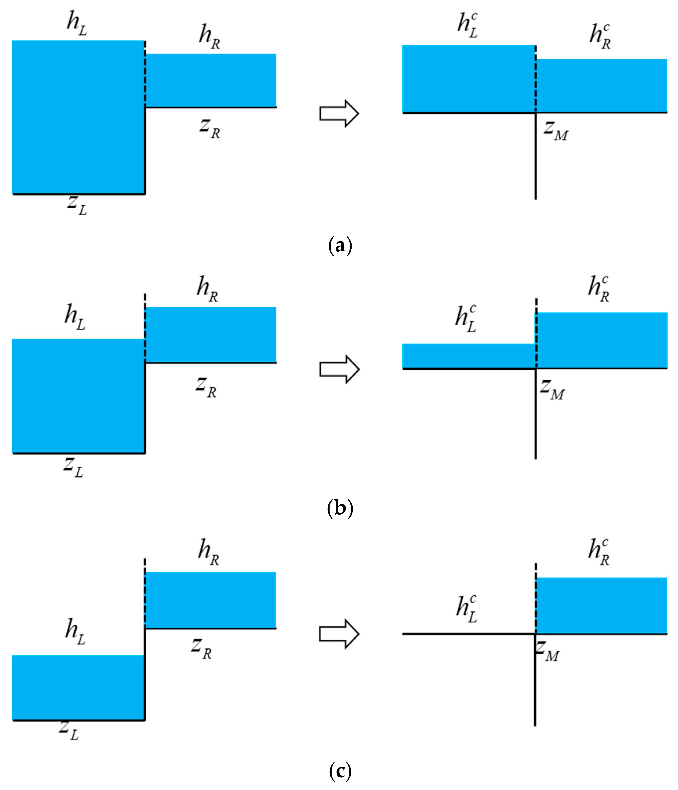
3.2. Water Depth Reconstruction

The numerical stability of the hydrodynamic model depends on the correct evaluation of the numerical flux and the bottom slope source term. It is important to the wet–dry front that one side of the interface has water and the others do not. Especially in the case water flows from a wet grid to a dry grid over complex terrain, reasonable evaluation of numerical flux is essential for numerical stability. The hydrostatic reconstruction (HR) method presented by Audusse et al. [23] is an efficient and robust method. The flow variables are reconstructed using the assessed water depth and bottom elevation at both sides. The HR method reconstructs the flow variables in the following steps.
At first, the maximum bottom elevation at both sides of the interface is defined as that in Audusse et al. [23]:
z M = max ( z L , z R ) .
Secondly, the reconstructed water depths at both sides are presented as:
h L c = max ( 0 , h L + z L z M ) h R c = max ( 0 , h R + z R z M ) .
Then, the velocities at both sides are in turn reconstructed as:
u d c = { u d , if   h d > h ε 0 , if   h d h ε v d c = { v d , if   h d > h ε 0 , if   h d h ε .
Without losing generality, Figure 2 indicates three cases where two cells share a common edge at the discrete level. The water depths of the two cells are reconstructed above the maximum bottom elevation. Peculiarly, if the water level of a cell is less than the bottom elevation of another cell, then its water depth is reconstructed as zero, as illustrated in Figure 2c.

3.3. Interface Numerical Flux and Slope Source Term Discretization

The SWEs are solved using a Godunov-type finite volume scheme in this model. The interfaces flux is calculated by solve Riemann problem. However, it is difficult to calculate the analytical solution to the Riemann problem quickly due to the large amount of computation cost. In the current work, the HLLC approximate Riemann solver [17] is used to calculate the numerical flux at the interface. The Riemann problem only requires solving once at each edge to detect the numerical flux at the cell interface using Equation (7)−(10). The interface flux is calculated using the reconstructed variables in Section 3.2, and the flux is given by the HLLC approximate Riemann solver as:
F = { F L if S L > 0 F L * if S L 0 S M F R * if S M 0 S R F R if S R 0
where F L = F ( U L ) and F R = F ( U R ) represent the calculated Riemann states from the left and right; SL, SR, and SM refer to characteristic wave speeds; and F L * and F R * indicate the numerical fluxes in the left and right middle regions of the HLLC approximate Riemannian solver in the solution structure, given by
F L * = [ F 1 * F 2 * v L F 1 * ] , F R * = [ F 1 * F 2 * v R F 1 * ]
with the HLL fluxes calculated by
F * = S R F L S L F R + S L S R ( U R U L ) S R S L .
The left and right characteristic waves are defined as:
S L = { u R 2 g h R , if h L = 0 min ( u L g h L , u * g h * ) , if h L > 0 S R = { u L + 2 g h L , if h R = 0 max ( u R + g h R , u * + g h * ) , if h R > 0
with
u * = 1 2 ( u L + u R ) + g h L g h R h * = 1 g [ 1 2 ( g h L + g h R ) + 1 4 ( u L u R ) ] 2
Then, the middle characteristic wave speed is calculated:
S M = S L h R ( u R S R ) S R h L ( u L S L ) h R ( u R S R ) h L ( u L S L )
Following the recommendation by Audusse et al. [23], the bottom slope source term at the cell interface can be solved as:
S b L = 1 2 g ( h L c 2 h L 2 )
and the bottom slope source term of the cell is given by
S b i = 1 Ω i k = 1 N E S b k , i l k , i [ 0 n x k n y k ] i

3.4. Friction Source Term

A splitting point-implicit method [9,24,33] is adopted to evaluate the friction source term in the present study. This method is equivalent to addressing the following ordinary differential equations
d U d t = S f ,
where S f = [ 0 S f x S f y ] T , and
S f x = C f u u 2 + v 2 S f y = C f v u 2 + v 2 .
Taking the x-direction as an instance in Equation (22), S f x can be expanded using a Taylor series as:
S f x n + 1 = S f x n + ( S f x U x ) Δ U x + o ( Δ U x 2 ) ,
in which Δ U x = U x n + 1 U x n . Ignoring the higher-order terms, together with Equation (24), Equation (22) is rewritten as:
U x n + 1 = U x n + Δ t ( S f x D x ) n = U x n + Δ t S ¯ f x
where Dx is implicit coefficient defined as:
D x = 1 + Δ t ( S f x U x ) n
and S ¯ f x refers to the implicit friction source term. The greatest effect of friction on the flow is to reduce the flow velocity to 0. To avoid an unphysical velocity, S ¯ f x is limited as follows:
S ¯ f x { q x n / Δ t if q x n 0 q x n / Δ t if q x n 0
Due to this limitation, friction can no longer change flow direction.

3.5. Rainfall and Infiltration Source Term

The rain and infiltration source terms are simply calculated by
h i n + 1 = h i n + R i + I i
where Ri is the rainfall rate in cell i and Ii is the infiltration rate calculated by the Horton method as:
f = f c + ( f 0 f c ) e β t
in which f0 and fc are the maximum and stable infiltration rates, respectively; β is the recession coefficient; and t represents the infiltration duration.

3.6. Stability Criteria

The stability of explicit numerical scheme can be governed by the Courant–Friedrichs–Lewy (CFL) criterion. In terms of all edges, the time step may be presented as:
Δ t = CFL min k [ min ( d L , d R ) max ( u L + g h L , u R + g h R ) ] k
where CFL is a value between 0 and 1 and d suggests the distance from a cell’s center to its edge.

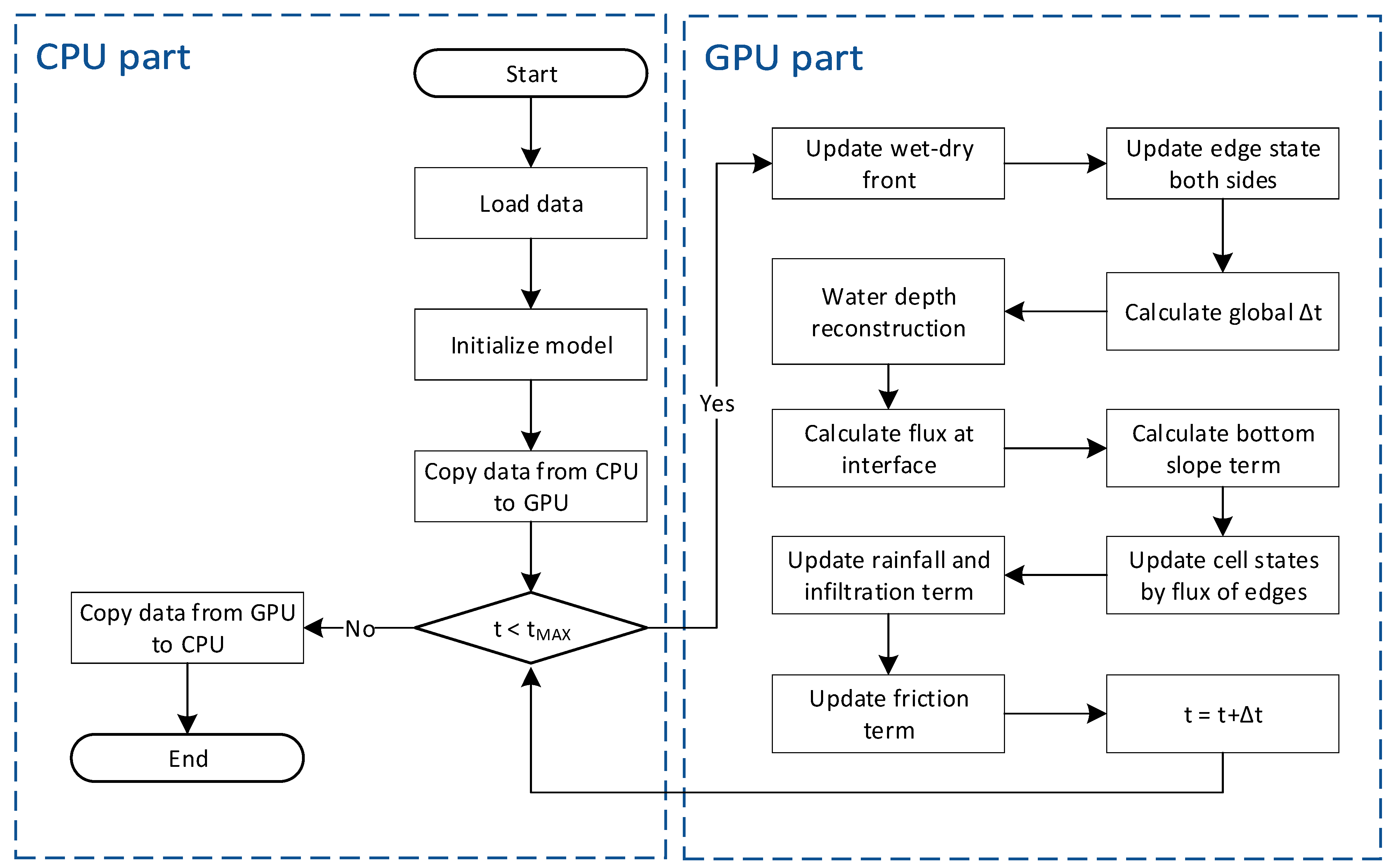
3.7. GPU-Accelerated Procedure

Graphics processing units (GPUs) have become a popular choice for scientific computations, artificial intelligence, and other high-performance computing applications due to their remarkable parallel processing capabilities. Furthermore, the use of GPUs has also led to notable advancements in the field of hydrodynamic numerical simulations, which are computationally expensive. Among the prominent GPU programming languages, including CUDA, OpenCL, and OpenAcc, CUDA is adopted in this work due to its high computational efficiency. We have employed a C-style CUDA programming language, utilizing standard I/O and mathematical libraries for the I/O file and numerical calculations, respectively. The model’s workflow involves the CPU controlling the I/O and computation process while the GPU performs the numerical simulation calculations.
Upon reading the grid topology information and parameters, the CPU transfers all the relevant data from the CPU memory to the GPU memory. All topology information and parameters are stored in the GPU’s global memory, which can be accessed by all threads. During the numerical computation in the GPU, appropriate threads are allocated to meet the model’s calculation requirements. The thread allocation parameters in CUDA are composed of two components, a grid and block. Variables of all threads in a block can access each other, and they are computed in a group of at least 32 threads. In this study, we have used the thread parameters of grid 128 and block 256. In each computed term, variables are copied from global memory to the thread’s local memory. These variables are utilized to evaluate the current item. As an illustration, for the calculation of water depth reconstruction, we compute the water depth and velocity of reconstruction on both sides of the edge. To achieve this, the grid parameters of the current edge of the modification thread are first copied to the local memory. These parameters include the index of the units on both sides of the edge, the water flow parameters of the units, and the bottom slope elevation. Then, the reconstructed flow variables are calculated by Equations (11)–(13). Finally, the results are copied to the global memory used for storing the reconstructed flow variables, which will be used for the subsequent interface flux calculation.
Figure 3 presents the procedure of implementing the proposed multi-threading approach for GPU parallel computing. At each time step, the model first evaluates the wet and dry states to determine the wet grid and the dry–wet fronts for subsequent calculations. Next, the water depth variables on both sides of the edges are updated to calculate the local time step. The current updated time step is determined by taking the minimum value of the local time steps calculated by Equation (30). The flux of the edge is then calculated and updated into the cells. Finally, the rainfall, infiltration, and friction source terms are updated. The aforementioned procedures are repeated in each time step until the set maximum simulation time is reached. In addition, at the end of the simulation, the data will be copied from the GPU memory to the CPU memory for writing and post-processing, if necessary, at any moment during the simulation.

4. Model Validation and Results

4.1. Still Water Test in an Uneven Bed

Well-balanced and conservative properties are essential for hydrodynamic models for it to be able to maintain the static state of the water level in the study area and not generate spurious flow velocities in still water conditions. With the purpose of validating the present 2D overland flow model, a still, steady flow over uneven terrain with a wet–dry interface is considered [33]. There are two overlapping bumps in the terrain, which are as set by d ( x , y ) = max ( 0 , D 1 , D 2 ) , where D 1 = 2000 0.0032 [ ( X 3000 ) 2 + ( Y 5000 ) 2 ] and D 2 = 900 0.000144 [ ( X 5000 ) 2 + ( Y 3000 ) 2 ] . The domain of 8000 m × 8000 m is divided into 58,672 cells. In addition, this domain is set as the initial water level of 1000 m. The simulation result at T = 5000 s is shown in Figure 4, the water level remains the same as the initial water level with no velocity, clearly revealing that the lake at rest can be recreated in an exact way. The results show that the model strictly maintains the C-property for the still water case with the presence of wet–dry fronts.

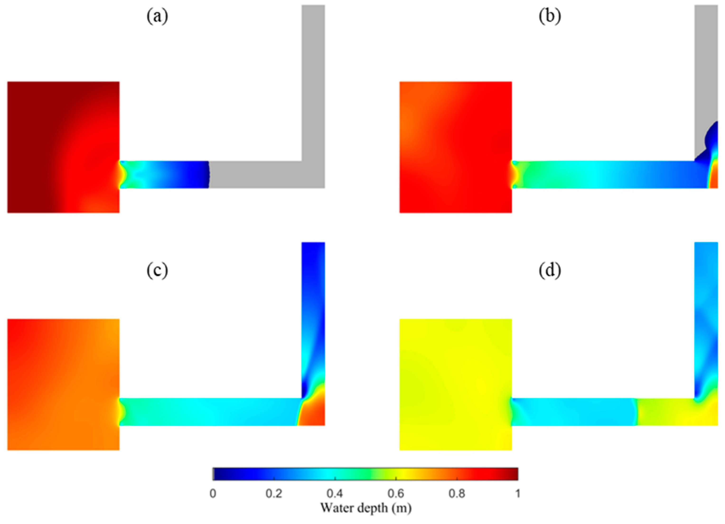
4.2. Dam-Break Flow in a 90° Curved Channel

A good shock-capturing capability is important to numerical simulation. A dam-break flow in a 90° curved channel is considered to validate the present model’s shock-capturing capability [34]. Concerning this test case, the domain is displayed as in Figure 5 [35], and it forms a square reservoir feeding an L-shaped channel. The domain is composed of a 2.4 × 2.4 m square water reservoir and an L-shaped, 90° curved river channel, which is divided into 113,796 cells. The numbering names of the six measured points and their location divisions are at points as shown in Figure 5 and Table 1, respectively. A uniform Manning coefficient is used for this domain, which is set as 0.0095 s·m−1/3. In addition, the zero bottom elevation was applied in this domain. The initial conditions include zero flow and 0.2 m depth in the reservoir and 0.0 m in the channel. Meanwhile, the whole domain is closed, except the outlet, which is regarded to be open.
The contour plot of the depth at t = 1 s, 3 s, 5 s, and 10 s is displayed in Figure 6a–d, respectively. The contour plot results can directly reflect the water resistance at the straight corner of the river channel. In this case, the dam breaks at the beginning of the simulation, and an overland flow model simulates the water flow processes within 40s. Meanwhile, the calculated water depth with six measured points is compared with the experimental data, as shown in Figure 7. The simulated water depths have good consistency with the measured water depth at the six measured points. In particular, the model accurately predicts the flood water arrival time of each measured point downstream. In addition, the simulation results of this model were compared with the results by Gottardi et al. [34], and our results have better agreement with the measured results than Gottardi’s results.
At the same time, as shown in Figure 7, the water level rose rapidly twice at three measured points, which are P2, P3, and P4. These measured points are all located in the river between the dam and the 90° bend of the channel. For these points, the direct cause of the first rapid rise in water level was due to the sudden downward discharge of the water body after the dam breaks. Meanwhile, the second rapid rise in the water level was due to water being blocked at the turn of the straight angle of the river channel. On the other side, the water level just rose rapidly once for two points, which are P5 and P6. This is caused by these two points not being directly affected by the water blocking occurring at the straight corner bend of the channel. Thus, these two points rose rapidly once, and the water depth became low as the water flowed out of the calculation domain. The simulation results show that the model can capture shocks in flows following dam breaks well.

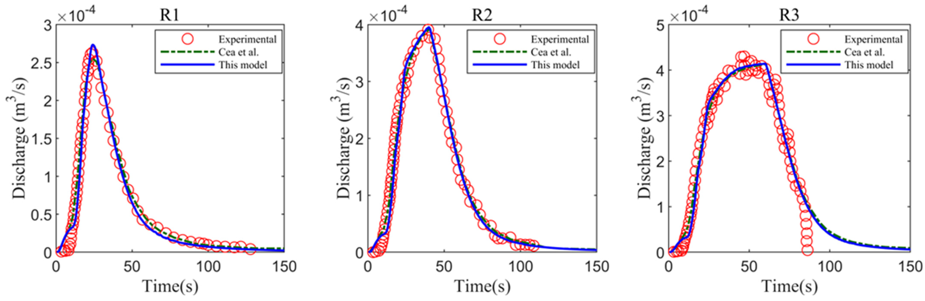
4.3. Urban Rainfall Runoff Experiment

Urban rainfall-runoff-induced overland flows are difficult to simulate two-dimensionally in urban areas, for example, due to their unsteady wet–dry interface and low water depth. To validate the current 2D overland model of rainfall-runoff-induced flow in an urban area, experiments on the rainfall runoff in an experimental urban area performed by Cea et al. [36,37] can be adopted. The catchment topography in shown in Figure 8, which gradually decreases from the outside region into inside region. Meanwhile, the domain mesh has a random placement, as shown in Figure 9. In addition, buildings are shown by wood blocks of 20 cm × 30 cm and 20 cm in height. Moreover, three rainfall events, set as R1, R2, and R3, applied a uniform rainfall supply rate of 25 L/min over 20, 40, and 60 s, respectively, to yield a rainfall intensity of 300 mm/h (Table 2). The whole area was discretized with unstructured grids and divided into 113,796 cells. A uniform Manning coefficient is used for this domain, which is set as 0.013 s·m−1/3. The calculated outlet discharges in three rainfall events are compared based on the experimental data [5], as shown in Figure 10. The simulated and measured outlet discharges exhibit good consistency. In addition, the present results are compared with the simulation results by Cea et al. [36], and the present model has almost the same results as their study. This case study shows that the present model has a good accuracy in the simulation of the rainfall-runoff process in urban areas.
Clearly, the simulated water depth and flow patterns at 20, 40, and 60 s in three rainfall events are displayed in Figure 11. It is clear that domain terrain plays a key role in the rainfall-runoff process and the consequent flow patterns. Rainwater flows from the buildings’ sloping roofs to the ground, where it is directed to the valley in the basin’s center and travels to the bottom outlet. In addition, this case study reveals that the present overland flow can simulate the rainfall-induced overland flow in the urban area well, taking into account the blocking effect of urban buildings. All in all, the present model can deal well with unsteady wet–dry interfaces and low water depths in the numerical simulation of urban areas.

4.4. Experiment of a Flash Flood over Urban Topography

In urban areas, there are a large number of buildings, which affects surface flow. A lot of physical experiments have been conducted to investigate the propagation characteristics of flood waves flowing into the urban area in Toce Valley. To validate the performance of current the 2D model in an urban area, a flash flood in Toce river can be adopted [38]. Numerous physical experiments are conducted with two topography configurations, two types of block arrangements (aligned and random), and three different inflow hydrographs. In this study, we select buildings in the aligned layout, as shown in Figure 12a. The buildings are shown by 15 cm concrete cubes. Ten gauges (P1–P10) have been placed at crucial locations to measure the water depth. The whole area was discretized with unstructured grids and divided into 30,319 cells. A uniform Manning coefficient is used for this domain, which is set as 0.0162 s·m−1/3. In addition, the low inflow hydrograph has been applied to this configuration, which was controlled by a pump located at the upstream of the valley, as shown in Figure 12b. The initial conditions include zero water depth in the whole domain and the downstream of the valley set as an open boundary.
The water depths and water velocities predicted by the model at different times are shown in Figure 13. The results shown in this figure clearly demonstrate the model’s ability to capture the instantaneous flow of the flash flood and reflect the water blocking effect of buildings. Before the flow arrives at the buildings, the flood front is moving at a fast speed. However, the water flow was delayed by buildings, which causes water deflection and flow alteration. In the meantime, a large part of the flood flows down the two edges of the valley and avoids the building area. The water depths decrease after the flood peak reduces.
The calculated water depths at nine gauges are shown in Figure 14. The simulated results have good consistency with the measured results. Meanwhile, the simulation results can almost accurately predict the arrival time of the peak and maximum water depths. Comparison of the calculated and measured water depths at P5 showed a slight difference. This result might due to the SWEs being unable to account for the three-dimensional transient and turbulent water flow. All in all, this case study reveals that the present overland model can simulate the inflow-induced overland flow of water in an urban area well, accounting for the blocking effect of urban buildings.

4.5. Malpasset Dam Break

The Malpasset dam, which was built in the southern French river valley of the Reyran, gave way in 1959 as a result of heavy rain. Due to its more detailed measured, experimental, and topographic data, this study area is widely used to test the accuracy and stability of two-dimensional mathematical models and their ability to deal with real terrain [39,40,41]. Here, a dam-break flow in Malpasset is considered to validate the present model’s performance in a large-scale and real case. The terrain data and the measured data were provided as shown in Figure 15. There are 17 measurement points of actual investigation (P1~P17), 9 measured points (G6~G14) in the physical experiment, and 3 transformers (A, B, and C) located downstream of the dam. The whole area was discretized with unstructured grids and divided into 275,476 cells. A uniform Manning coefficient is used for this domain, which is set as 0. 033 s·m−1/3. In addition, the initial conditions include a 100 m water level upstream of the dam and zero water level in the studied area.
The contour plot of water depth at t = 2000 s is displayed in Figure 16 when the wave front had already reached the downstream floodplain. In other words, the contour plot results can directly reflect the water from the dam break reaching the downstream area of the floodplain. A comparison of the calculated and measured results is shown in Figure 17a–c, which includes the survey and the experimental observations in terms of maximum water levels and wave arrival times. Meanwhile, the estimated model results and the measured and experimental values exhibit good consistency. The uncertainty of the survey and experimental data may lead to some differences in some measurement points. These discrepancies may be attributed to the 2D model’s limitations in the simulation of a 3D flow, some measurement uncertainties in the survey and experiment, changes in the topography after the initial event, as well as scale effects in the experiment, particularly for the roughness. However, the present results are compared with the simulation results by Hou et al. [33] and Nikolos et al. [42], and the present model has almost the same results as their simulation results. This case study shows that the present model has a good accuracy in the simulation of the dam break. All in all, the present overland model can deal with unsteady wet–dry interfaces and uneven bed numerical simulation problems well in a real dam-break case and can thus accurately predict the dam-break flow for large-scale applications.
This case aims to evaluate the efficiency of the present model using different hardware configurations. The statistics of computational cost with different hardware configurations are shown in Table 3. These statistics show that a multi-core GPU is more efficient than other hardware configurations. Specially, the efficiencies of the GPU and CPU devices are compared in this table. This model can achieve a speeding up ratio of around 4 using 10-core CPUs compared to a single-thread CPU. With the GPU computation framework, this model can achieve around a 75 speeding up ratio compared to a single thread CPU in the dam-break flow for a large-scale application. Here, the computational efficiency of a GPU with multiple CUDA cores is appreciably higher than that of a multi-core CPU.

5. Conclusions

A new 2D, unstructured, grid-based hydrodynamic model with conservation and balance properties is presented in this paper. This model is constructed using a Godunov-type finite volume scheme, which is able to deal with complex flows such as unsteady wet–dry interfaces, low water depths and uneven beds. More importantly, this new model is able to adopt GPUs to achieve numerical simulation of large-scale applications.
Five test cases have been adopted to validate the present model’s performance. The well-balanced and conservative properties have been proven by means of the still water test in an uneven bed. The model’s good shock-capturing capability has been validated by simulating a dam break in a 90° curved channel, which showed better agreement with the measured results than Gottardi’s results. This urban rainfall runoff experiment case shows that the present model has a good accuracy in the simulation of rainfall-runoff processes in urban area, which has almost the same results as Cea’s study and measured values. A case study of a flash flood over an urban topography revealed that the present overland model can simulate the inflow-induced overland flow in an urban area well, in which the blocking effect of urban buildings is taken into account. Finally, the Malpasset dam break case showed that the present model can deal with the numerical simulation of an unsteady wet–dry interface and an uneven bed in a real dam break case. The simulation results show that the numerical methods used are reliable and effective. The model has considerable predictive potential for complex flows in rainfall runoff, river hydraulics and inundation, dam breaks, and other flood processes.
The numerical simulation of the Malpasset dam break further demonstrated the efficiency of the present model using different hardware configurations. The use of a GPU is much more efficient than a multi-core CPU. Particularly, the ratio of a 10-core CPU is 3.76, while the ratio of a CPU with multiple CUDA cores can be as high as 74.47. The hydrodynamic model on the basis of the GPU framework shows a powerful computing advantage in processing a large number of grids with high resolution. The model adopts a method which is easier to implement and more robust in the calculation of some terms and that can be flexibly implemented to improve each term under the current GPU framework.

Author Contributions

Conceptualization, F.C.; methodology, F.P. and X.H.; validation, F.P. and F.C.; data curation, F.C.; writing—original draft preparation, F.P.; writing—review and editing, X.H. and F.C. All authors have read and agreed to the published version of the manuscript.

Funding

This research was funded by the National Key Research and Development Program of China (2016YFC0803107), Beijing Science and Technology Project (No. Z201100008220005).

Data Availability Statement

No new data were created or analyzed in this study. Data sharing is not applicable to this article.

Acknowledgments

The authors would like to extend our deepest gratitude to Hongping Zhang and Guangyuan Kan for their invaluable help and support in this work.

Conflicts of Interest

The authors declare no conflict of interest.

References

  1. Li, S.; Duffy, C.J. Fully coupled approach to modeling shallow water flow, sediment transport, and bed evolution in rivers. Water Resour. Res. 2011, 47, W03508. [Google Scholar] [CrossRef]
  2. Aricò, C.; Sinagra, S.; Begnudelli, L.; Tucciarelli, T. MAST-2D diffusive model for flood prediction on domains with triangular Delaunay unstructured meshes. Adv. Water Resour. 2011, 34, 1427–1449. [Google Scholar] [CrossRef] [Green Version]
  3. Benkhaldoun, F.; Sahmim, S.; Sea, D.M. A two-dimensional finite volume morphodynamic model on unstructured triangular grids. Int. J. Numer. Methods Fluids 2010, 63, 1296–1327. [Google Scholar] [CrossRef]
  4. Canestrelli, A.; Fagherazzi, S.; Lanzoni, S. A mass-conservative centered finite volume model for solving two-dimensional two-layer shallow water equations for fluid mud propagation over varying topography and dry areas. Adv. Water Resour. 2012, 40, 54–70. [Google Scholar] [CrossRef]
  5. Fiedler, F.R.; Ramirez, J.A. A numerical method for simulating discontinuous shallow flow over an infiltrating surface. Int. J. Numer. Methods Fluids 2000, 32, 219–239. [Google Scholar] [CrossRef]
  6. Song, L.; Zhou, J.; Guo, J.; Zou, Q.; Liu, Y. A robust well-balanced finite volume model for shallow water flows with wetting and drying over irregular terrain. Adv. Water Resour. 2011, 34, 915–932. [Google Scholar] [CrossRef]
  7. Simons, F.; Busse, T.; Hou, J.; Özgen, I.; Hinkelmann, R. A model for overland flow and associated processes within the Hydroinformatics Modelling System. J. Hydroinformatics 2014, 16, 375–391. [Google Scholar] [CrossRef]
  8. Yu, C.; Duan, J. Two-dimensional hydrodynamic model for surface-flow routing. J. Hydraul. Eng. 2014, 140, 04014045. [Google Scholar] [CrossRef]
  9. Zhang, H.; Wu, W.; Hu, C.; Hu, C.; Li, M.; Hao, X.; Liu, S. A distributed hydrodynamic model for urban storm flood risk assessment. J. Hydrol. 2021, 600, 126513. [Google Scholar] [CrossRef]
  10. Toro, E.F.; Garcia-Navarro, P. Godunov-type methods for free-surface shallow flows: A review. J. Hydraul. Res. 2007, 45, 736–751. [Google Scholar] [CrossRef]
  11. LeVeque, R.J. Balancing source terms and flux gradients in high-resolution Godunov methods: The quasi-steady wave-propagation algorithm. J. Comput. Phys. 1998, 146, 346–365. [Google Scholar] [CrossRef] [Green Version]
  12. Zhang, D.; Quan, J.; Wang, Z.; Zhang, H.; Ma, J. Numerical Simulation of Overland Flows Using Godunov Scheme Based on Finite Volume Method. EPiC Ser. Eng. 2018, 3, 2425–2432. [Google Scholar]
  13. LeFloch, P.G.; Thanh, M.D. A Godunov-type method for the shallow water equations with discontinuous topography in the resonant regime. J. Comput. Phys. 2011, 230, 7631–7660. [Google Scholar] [CrossRef] [Green Version]
  14. Brufau, P.; Garcia-Navarro, P. Two-dimensional dam break flow simulation. Int. J. Numer. Methods Fluids 2000, 33, 35–57. [Google Scholar] [CrossRef]
  15. George, D.L. Augmented Riemann solvers for the shallow water equations over variable topography with steady states and inundation. J. Comput. Phys. 2008, 227, 3089–3113. [Google Scholar] [CrossRef]
  16. Harten, A.; Lax, P.D.; Leer, B.V. On Upstream Differencing and Godunov-Type Schemes for Hyperbolic Conservation Laws. SIAM Rev. 1983, 25, 35–61. [Google Scholar] [CrossRef]
  17. Toro, E.F.; Spruce, M.; Speares, W. Restoration of the contact surface in the HLL-Riemann solver. Shock Waves 1994, 4, 25–34. [Google Scholar] [CrossRef]
  18. Murillo, J.; García-Navarro, P. Weak solutions for partial differential equations with source terms: Application to the shallow water equations. J. Comput. Phys. 2010, 229, 4327–4368. [Google Scholar] [CrossRef]
  19. Murillo, J.; García-Navarro, P. Augmented versions of the HLL and HLLC Riemann solvers including source terms in one and two dimensions for shallow flow applications. J. Comput. Phys. 2012, 231, 6861–6906. [Google Scholar] [CrossRef]
  20. Hou, J.; Liang, Q.; Simons, F.; Hinkelmann, R. A stable 2D unstructured shallow flow model for simulations of wetting and drying over rough terrains. Comput. Fluids 2013, 82, 132–147. [Google Scholar] [CrossRef]
  21. Marche, F.; Bonneton, P.; Fabrie, P.; Seguin, N. Evaluation of well-balanced bore-capturing schemes for 2D wetting and drying processes. Int. J. Numer. Methods Fluids 2007, 53, 867–894. [Google Scholar] [CrossRef]
  22. Song, L.; Zhou, J.; Li, Q.; Yang, X.; Zhang, Y. An unstructured finite volume model for dam-break floods with wet/dry fronts over complex topography. Int. J. Numer. Methods Fluids 2011, 67, 960–980. [Google Scholar] [CrossRef]
  23. Audusse, E.; Bouchut, F.; Bristeau, M.-O.; Klein, R.; Perthame, B.T. A Fast and Stable Well-Balanced Scheme with Hydrostatic Reconstruction for Shallow Water Flows. SIAM J. Sci. Comput. 2004, 25, 2050–2065. [Google Scholar] [CrossRef] [Green Version]
  24. Liang, Q.; Marche, F. Numerical resolution of well-balanced shallow water equations with complex source terms. Adv. Water Resour. 2009, 32, 873–884. [Google Scholar] [CrossRef]
  25. Xia, X.; Liang, Q.; Ming, X.; Hou, J. An efficient and stable hydrodynamic model with novel source term discretization schemes for overland flow and flood simulations. Water Resour. Res. 2017, 53, 3730–3759. [Google Scholar] [CrossRef]
  26. Horritt, M.S.; Bates, P.D. Effects of spatial resolution on a raster based model of flood flow. J. Hydrol. 2001, 253, 239–249. [Google Scholar] [CrossRef]
  27. Brown, J.D.; Spencer, T.; Moeller, I. Modeling storm surge flooding of an urban area with particular reference to modeling uncertainties: A case study of Canvey Island, United Kingdom. Water Resour. Res. 2007, 43, W06402. [Google Scholar] [CrossRef] [Green Version]
  28. Huxley, C. Rapid and Accurate Storm Water Drainage System Assessments Using GPU Technology; BMT: Brisbane, Australia, 2017. [Google Scholar]
  29. Fewtrell, T.; Bates, P.D.; Horritt, M.; Hunter, N. Evaluating the effect of scale in flood inundation modelling in urban environments. Hydrol. Process. Int. J. 2008, 22, 5107–5118. [Google Scholar] [CrossRef]
  30. Leandro, J.; Chen, A.S.; Schumann, A. A 2D parallel diffusive wave model for floodplain inundation with variable time step (P-DWave). J. Hydrol. 2014, 517, 250–259. [Google Scholar] [CrossRef]
  31. Wu, Y.; Tian, L.; Rubinato, M.; Gu, S.; Yu, T.; Xu, Z.; Cao, P.; Wang, X.; Zhao, Q. A New Parallel Framework of SPH-SWE for Dam Break Simulation Based on OpenMP. Water 2020, 12, 1395. [Google Scholar] [CrossRef]
  32. Xia, X.; Liang, Q.; Ming, X. A full-scale fluvial flood modelling framework based on a high-performance integrated hydrodynamic modelling system (HiPIMS). Adv. Water Resour. 2019, 132, 103392. [Google Scholar] [CrossRef]
  33. Hou, J.; Liang, Q.; Simons, F.; Hinkelmann, R. A 2D well-balanced shallow flow model for unstructured grids with novel slope source term treatment. Adv. Water Resour. 2013, 52, 107–131. [Google Scholar] [CrossRef]
  34. Gottardi, G.; Venutelli, M. Central scheme for two-dimensional dam-break flow simulation. Adv. Water Resour. 2004, 27, 259–268. [Google Scholar] [CrossRef]
  35. Frazão, S.S.; Zech, Y. Dam Break in Channels with 90° Bend. J. Hydraul. Eng. 2002, 128, 956–968. [Google Scholar] [CrossRef]
  36. Cea, L.; Garrido, M.; Puertas, J. Experimental validation of two-dimensional depth-averaged models for forecasting rainfall–runoff from precipitation data in urban areas. J. Hydrol. 2010, 382, 88–102. [Google Scholar] [CrossRef]
  37. Cea, L.; Garrido, M.; Puertas, J.; Jácome, A.; Del Río, H.; Suárez, J. Overland flow computations in urban and industrial catchments from direct precipitation data using a two-dimensional shallow water model. Water Sci. Technol. J. Int. Assoc. Water Pollut. Res. 2010, 62, 1998–2008. [Google Scholar] [CrossRef]
  38. Testa, G.; Zuccala, D.; Alcrudo, F.; Mulet, J.; Soares-Frazão, S. Flash flood flow experiment in a simplified urban district. J. Hydraul. Res. 2007, 45, 37–44. [Google Scholar] [CrossRef]
  39. Goutal, N. The Malpasset dam failure. An overview and test case definition. In Proceedings of the 4th CADAM Meeting, Zaragoza, Spain, 18–19 November 1999; pp. 18–19. [Google Scholar]
  40. Yoon, T.H.; Kang, S.-K. Finite volume model for two-dimensional shallow water flows on unstructured grids. J. Hydraul. Eng. 2004, 130, 678–688. [Google Scholar] [CrossRef]
  41. George, D. Adaptive finite volume methods with well-balanced Riemann solvers for modeling floods in rugged terrain: Application to the Malpasset dam-break flood (France, 1959). Int. J. Numer. Methods Fluids 2011, 66, 1000–1018. [Google Scholar] [CrossRef]
  42. Nikolos, I.; Delis, A. An unstructured node-centered finite volume scheme for shallow water flows with wet–dry fronts over complex topography. Comput. Methods Appl. Mech. Eng. 2009, 198, 3723–3750. [Google Scholar] [CrossRef]
Figure 1. The cell topology of unstructured grids.
Water 15 01300 g001
Figure 2. Illustration of hydrostatic reconstruction at: (a) hL + zL > hR + zR; (b) hL + zL < hR + zR; and (c) hL + zL < zR.
Water 15 01300 g002
Figure 3. Multi-thread hydrodynamic numerical simulation process in GPU.
Water 15 01300 g003
Figure 4. Still water test in an uneven bed: results of the still water test at T = 5000 s. The blue color represents water level, and the other colors represent the elevation of the bottom slope.
Water 15 01300 g004
Figure 5. Dam-break flow in a 90° curved channel: schematic diagram in the 90° curved channel.
Water 15 01300 g005
Figure 6. Dam-break flow in a 90° curved channel: simulated water depth at t = 1, 3, 5, 10 s, as shown in (ad).
Water 15 01300 g006
Figure 7. Dam-break flow in a 90° curved channel: simulated and measured water depth [34].
Water 15 01300 g007
Figure 8. Urban rainfall-runoff experiment: topography of the experimental area.
Water 15 01300 g008
Figure 9. Urban rainfall-runoff experiment: mesh and representation of buildings (partial area). The blue color represents the normal sides, and the red color represent the building sides.
Water 15 01300 g009
Figure 10. Urban rainfall-runoff experiment: simulated and measured outlet discharges [36].
Water 15 01300 g010
Figure 11. Urban rainfall-runoff experiment: simulated water depths and flow patterns at the last moment of three rainfall events.
Water 15 01300 g011
Figure 12. Flash flood in an urban area: (a) layout of the physical model; (b) inflow hydrograph.
Water 15 01300 g012
Figure 13. Flash flood in an urban area: simulated water depths and velocities.
Water 15 01300 g013
Figure 14. Simulated and measured water depths at nine sample gauges.
Water 15 01300 g014
Figure 15. Malpasset dam break: topography and location of experimental points.
Water 15 01300 g015
Figure 16. Malpasset dam break: numerical flood routing at t = 2000 s.
Water 15 01300 g016
Figure 17. Malpasset dam break: comparison of numerical simulation results with observed and experimental results: (a) Maximum water level (survey points); (b) Maximum water level (scale model measurements); and (c) Wave arrival time (scale model measurements) [33,42].
Water 15 01300 g017
Table 1. Dam-break flow in a 90° curved channel: location of six measured points.
PointX (m)Y (m)
P11.201.20
P22.750.70
P34.250.70
P45.750.70
P56.551.50
P66.553.00
Table 2. Urban rainfall-runoff experiment: rainfall schemes.
Rainfall EventsRainfall Intensity
(mm/h)
Rainfall Duration
(s)
R130020
R230040
R330060
Table 3. Hardware configurations and computational cost for the Malpasset dam break.
HardwareHardware SetupHardware
Cores
Computational Cost (s)Speeding Up Ratio
CPUINTER i9-10900 111034.2351.00
2699.1981.48
4448.0422.31
6315.5803.28
8297.6813.47
10275.3723.76
GPUNVIDIA Geforce GTX 1660Ti 2 153677.21013.40
NVIDIA Geforce RTX 3070 Laptop 2512050.28320.57
NVIDIA RTX A4000 2614447.01222.00
NVIDIA Geforce RTX 3080Ti 210,24039.61226.11
NVIDIA Geforce RTX 3090 210,49635.71828.96
NVIDIA Geforce RTX 4090 216,38413.88874.47
1 Intel Corporation, Santa Clara, USA; 2 NVIDIA Corporation, Santa Clara, USA.
Disclaimer/Publisher’s Note: The statements, opinions and data contained in all publications are solely those of the individual author(s) and contributor(s) and not of MDPI and/or the editor(s). MDPI and/or the editor(s) disclaim responsibility for any injury to people or property resulting from any ideas, methods, instructions or products referred to in the content.

