Article

Assessing the Extent of Flood-Prone Areas in a South-American Megacity Using Different High Resolution DTMs

by
Elton Vicente Escobar-Silva
1,*,
Cláudia Maria de Almeida
1,
Gustavo Barbosa Lima da Silva
2,
Ingobert Bursteinas
3,
Kleber Lopes da Rocha Filho
4,
Cleber Gonzales de Oliveira
5,
Marina Refatti Fagundes
6 and
Rodrigo Cauduro Dias de Paiva
6
1
Earth Observation and Geoinformatics Division, National Institute for Space Research (INPE), Sao Jose dos Campos 12227-010, SP, Brazil
2
Civil and Environmental Engineering Department, Technology Center, Federal University of Paraiba (UFPB), Joao Pessoa 58051-900, PB, Brazil
3
Civil Defense of Sao Caetano do Sul, Sao Caetano do Sul 09561-000, SP, Brazil
4
Flood Alert System of Sao Paulo (SAISP), Sao Paulo 05508-020, SP, Brazil
5
VISIONA Space Technology, Sao Jose dos Campos 12247-016, SP, Brazil
6
Institute of Hydraulic Research, Federal University of Rio Grande do Sul (UFRGS), Porto Alegre 91501-970, RS, Brazil
*
Author to whom correspondence should be addressed.
Water 2023, 15(6), 1127; https://doi.org/10.3390/w15061127
Submission received: 5 February 2023 / Revised: 2 March 2023 / Accepted: 8 March 2023 / Published: 15 March 2023
(This article belongs to the Section Hydraulics and Hydrodynamics)

Abstract

:
Current forecasts estimate that almost 68% of the global population will be living in urban centers by 2050. As a result, the increase in impermeable surface area can result in severe hydrological impacts, such as the increase in surface runoff and the frequency of floods and their magnitude. Thus, this work analyzes the performance of the hydrodynamic model HEC-RAS for assessing the extent of flood-prone areas, using two digital terrain models (DTM) with different spatial resolutions (5 and 0.50 m). Four different computing intervals (1, 15, 30, and 60 s) were adopted aiming to evaluate the simulations outputs performance. Additionally, reported data by the civil defense are used for calibration and validation. In general, the model showed to be a powerful tool in the identification of susceptible areas to urban flooding. The simulated results in this work provide crucial geographic information when identifying spots with the highest risk of flooding, which should receive priority attention during such events. The simulations with a spatial resolution of 5 m showed the flood maps with the largest coverage of the flooded points (278 points out of 286—97.20%), within the shortest computation times. We highlight that the more refined DTM derived from spatial images did not produce the best flood simulation compared to the DTM with a spatial resolution of 5 m derived from orthoimages.

1. Introduction

According to the United Nations (UN), the world’s population reached 8 billion people in 2022 [1], with 55% living in urban areas [2]. By 2050, current forecasts estimate that the global population will grow to 9.7 billion people [1], and the world’s city dwellers are expected to be 6.6 billion people (nearly 68% of the world’s population) [3]. On the other hand, the current urban sprawl rate is twice as fast as its population growth rate [4]. If the long-term urban expansion trend continues, the global area covered by urban settlements is expected to increase to over 3 million km2 by 2050, which would be equivalent to the entire country of India [5].
Unplanned or inappropriate management of rapid urban expansion and fast population growth can seriously increase environmental problems [6] in both physical and biological environments. From the physical environmental perspective, some of the most common modifications caused by urbanization involve land use and land cover change, increased impervious surface cover, and altered hydrology [7]. Increase in impervious surface areas result in severe hydrological impacts in urban areas. The clearest impacts of urban imperviousness on hydrological systems include reducing infiltration and hence a decrease in groundwater recharge [8]; increase in surface runoffs, in terms of speed, volumes, and peak flow [9]; and increase in flood frequency and its magnitude, especially in flood-prone areas [10].
Urban flooding represents a source of hazards for both developed and developing countries. It not only endangers human life, but also can cause property damage, mass migration, social and economic disruption, and environmental degradation [11]. Nearly 44% of disasters worldwide have been associated with floods, and different types of floods account for 31% of economic losses [12]. It is estimated that from 2001 to 2020 floods affected an average of 82.7 million people annually and caused a global annual average economic loss of US $34.1 billion [13]. To make things worse, urban flooding is expected to happen more often and severely as Earth experiences hydrometeorological extreme events driven by global climate change [14].
In Brazil, according to the Brazilian Atlas of Natural Disasters, from 1991 to 2012, floods were responsible for 73% of deaths related to natural disasters [15], and between 2000 and 2010 alone, floods killed 1200 people and caused economic losses of around US $2.8 billion [16]. From 2013 to 2021, at least 205 people were killed by floods and more than 11.7 million people were impacted by flooding events [17]. However, it is estimated that these numbers may be higher since (i) 90% of the 5570 municipalities reported the data associated with these events to the Brazilian Integrated Disaster Information System (S2iD) and (ii) only extreme events are reported to this database.
Urban flood risk assessment and management are fundamental steps for identifying current hazards and prone risk areas, and thus to mitigate the impacts in future flood events [18]. In this context, urban flood models (UFMs) are considered powerful tools to represent the features of urban ecosystems and the mechanisms of floods that impact them [19]. According to Neal et al. [20], UFMs could be grouped by simplified, hydrological, or hydrodynamic models. As its name suggests, simplified models use simplified equations to simulate the flooding process. Consequently, they neither consider physical processes simulation nor represent flow dynamics. A hydrological model can be defined as a mathematical representation of the water flow and its constituents over some part of the Earth’s surface and/or subsurface. This sort of model normally involves two main components: a rainfall–runoff estimator and a routing scheme. In its turn, a hydrodynamic model is a physical or mathematical representation of the fluid flow. These models simulate the movement of water, solving equations by applying laws of physics such as Navier–Stokes and Saint–Venant equations [20,21].
The urban hydrological modeling is a powerful tool for managing urban floods. Furthermore, in the last decade, modeling tools have improved significantly due to the development of computing techniques and the increased availability of high-resolution data. However, there is no universal methodology for urban hydrological modeling at the catchment scale due to the heterogeneity of urban areas and the great multiplicity of interactions between the urban structure and the water system [22]. Some of the most common difficulties associated with urban flood modeling are the unpredictable flow conditions in the urban environment due to rapid changes in topography and the unavailability of extensive raw data sets [23].
In this context, this work seeks to analyze the performance of the hydrodynamic model HEC-RAS for the identification and delimitation of urban areas susceptible to flood and maximum depth. Moreover, we investigate the role of different spatial resolutions in such simulations. To do so, two digital terrain models (DTM) with different resolutions are used. This study focuses on the analysis of floods hazard in São Caetano do Sul as a case study, which is part of the São Paulo megacity, the capital of São Paulo State located in the southeast of Brazil, using reported data by the civil defense of this municipality for both model calibration and validation.
It is worth mentioning that other works in the literature have dealt with the identification of flood-prone areas in nearby localities within the São Paulo Megacity. A flood risk map based on hydrological and mobility data was conceived for a sub-basin of the Tamanduateí River Watershed in a southeastern sector of São Paulo by [24]. As its input data, a flood susceptibility map was elaborated by means of the Height Above the Nearest Drainage (HAND) algorithm [25], using an SRTM DEM. The work jointly takes into account an exposure component, which regards the resident population and the population that works and studies in the analyzed area, and a vulnerability component that considers both a local vulnerability, assessed by previous records of floods in the area, and a network vulnerability, measured by the availability of alternative routes in the road network in the face of momentary hindrances. In this work, there is no simulation of flooding, and no rainfall data are employed either. The flood susceptibility map was generated by a slicing of the HAND output map.
Silva et al. [26] conducted flooding simulations for a sector of the Tamanduateí River Watershed in the central portion of São Paulo City, named Anhangabaú Lower Valley Sub-basin. The simulations were run employing the PCSWMM platform and relied on three alternative scenarios intended to mitigate the flooding problem in the lower valley. Initially, two flood detention reservoirs and a reinforcement of the main gallery system were envisaged to ensure safety against 25-year return period events. In a second scenario, a reinforcement of the main gallery and a flow derivation tunnel leading to Tamanduateí River were foreseen for a 100-year return period. The third scenario distributed linear retentions spread over the watershed considering stages of return periods of 10/25/100 years. The scenarios combined drainage system, urban occupancy, adoption of LID (Low Impact Development) controls, modeling dimension, and rainfall time series, and their evaluation regarded aspects such as alternative efficiency, prevented damages, permanent environmental impacts, temporary environmental impacts, costs, and public response. This work concerned prescriptive (hypothetical) and not real case simulations.
Another work in the same line was executed by [27], who conducted simulations in PCSWMM for six minor sub-basins in São Paulo City that experienced flood-related problems. The models were calibrated for each basin adopting recent extreme event data. The authors obtained as results profiles and hydrographs along simulated channels, reservoir states, flood inundation extents, and affected buildings. As this work was intended to act as a warning system, a PCSWMM Real-Time module was additionally conceived to disclose predictions for flood inundation sites based on radar rainfall forecasts, taken every 10 min to a prediction horizon of 3 h. These simulations were driven by only one DTM, and the groundwater modeling was disregarded due to the unavailability of tuning parameters. Likewise our findings, Oliveira et al. [27] pointed out that the model outputs are highly dependent on sufficient channels cross-section data and the DTM quality is decisive for an accurate delimitation of flooding areas.
Differently from the works described above, we have conducted simulations for a practical situation and carried out validations of our results relying on in situ data. Finally, we must say that our work aims not only to increase the scientific knowledge on this topic in the study area but also to provide a support tool to the civil defense agents and local decision-makers, as a means of building the capacity to enhance their readiness to prevent and mitigate the effects of such events.

2. Materials and Methods

2.1. Study Area

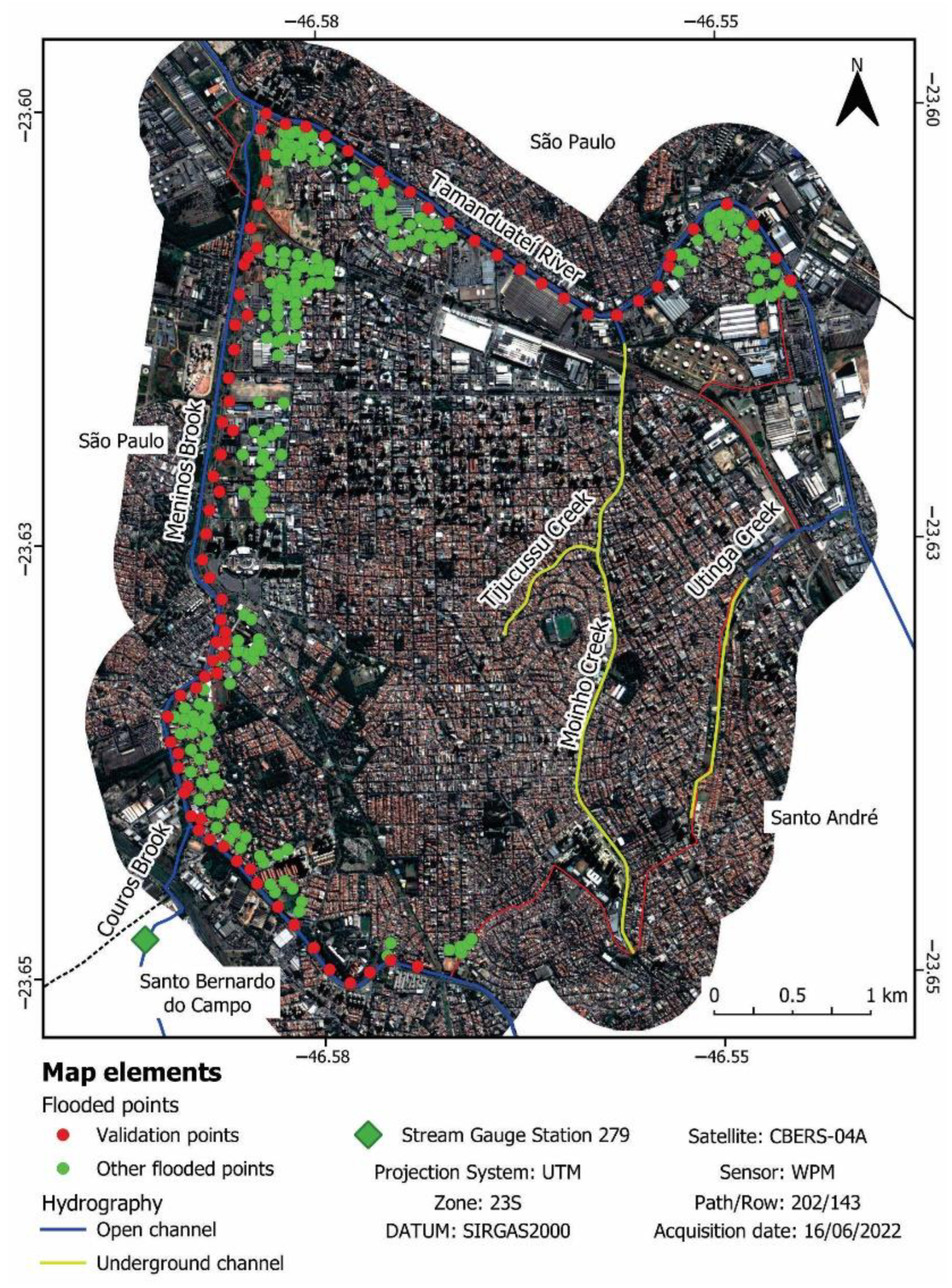
São Caetano do Sul is located in the southern São Paulo metropolitan area and belongs to an important industrial region in Brazil, named ABCD Region (Figure 1). The study site was chosen due to its history of floods (Table 1). The municipality is intensely conurbated with the municipalities of São Paulo, Santo André, and São Bernardo do Campo, with visually undefined limits among them. According to the Brazilian Institute of Geography and Statistics (IBGE), the current population of São Caetano do Sul is estimated at about 162,763 inhabitants in an area of 15.33 km2 [28]. São Caetano do Sul is the second city with the highest economic density [29] in the country and, according to the UN Sustainable Development Goals, the municipality occupies 1st place within the ranking of sustainable cities in Brazil [30].
The study area is situated on a plateau adjacent to a mountain chain named Serra do Mar (Portuguese term for “Sea Range”), with elevations ranging from 722 to 812 m above sea level and with a mean altitude of 758 m [31]. According to the Köppen climate classification [32], São Caetano do Sul has a humid subtropical climate (Cwa), with a mildly warm and rainy summer, and a moderate and dry winter. The average annual temperature is 19.5 °C, and the coldest and warmest months are July (average of 16.2 °C) and February (average of 22.5 °C), respectively [33]. The mean annual rainfall is 1496 mm, which was obtained from Station n° 2346051 of the Department of Water and Electricity (Departamento de Águas e Energia Elétrica—DAEE) of São Paulo State.
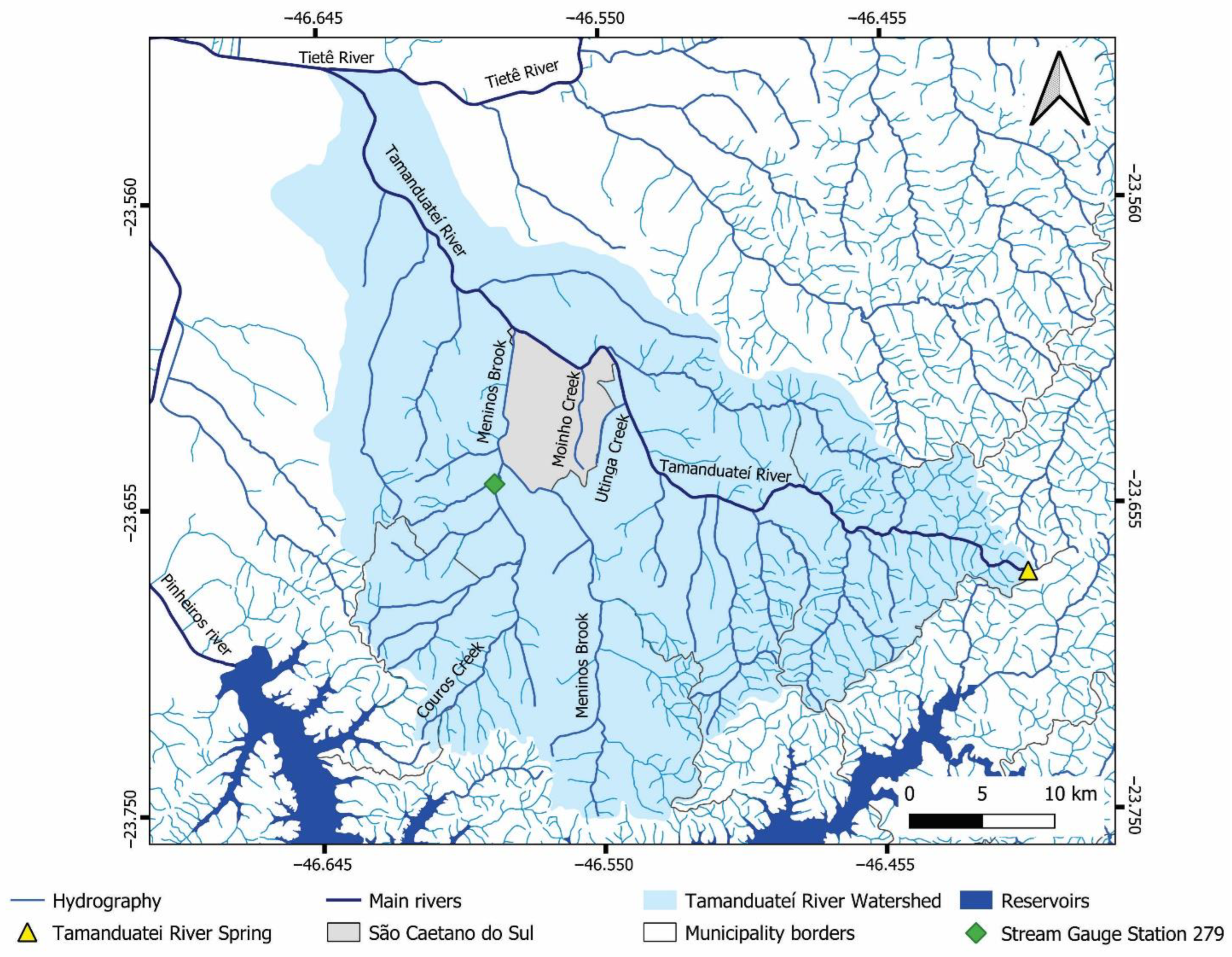
São Caetano do Sul is located downstream in the Tamanduateí River Watershed (Figure 2), a densely urbanized sub-basin of the Tietê Upstream River (Alto Tietê in Portuguese) Watershed. The Tamanduateí Watershed has a drainage area of 330.41 km2, which totally encompasses the city of São Caetano do Sul and partially the cities of Diadema, Mauá, Santo André, São Bernardo do Campo, and São Paulo. Its main river, Tamanduateí River, is 36.5 km long. Tamanduateí River rises in Mauá and flows into Tietê River by a narrow-rectified channel. The Tamanduateí River Watershed is divided into four sub-basins: Tamanduateí Inferior, which includes the city of São Paulo; Meninos Downstream and Couros; Tamanduateí Upstream and Meninos; and Tamanduateí Upstream and Oratorio, where its spring is located [34].

2.2. Case Study: The Extreme Event of March 2019

On 10 March 2019, São Caetano do Sul was devastated by severe widespread river floods and pondings (Figure 3 and Figure 4), resulting from an extreme rainfall of 179 mm in a period of 4 h [35]. The scenario was worsened due to river flows coming upstream from neighboring municipalities (Diadema, Mauá, Ribeirão Pires, Santo André, São Bernardo do Campo, and São Paulo), which caused the overflow of Tamanduateí River and Meninos Creek. According to the civil defense, nine neighborhoods were affected as follows: Centro, Cerâmica, Fundação, Jardim São Caetano, Mauá, Nova Gerty, Prosperidade, Santo Antônio, and São José. Approximately 2000 buildings were flooded and in more than half of them, the water depth reached almost 2 m in relation to the ground floor. In some neighborhoods, the water column reached 2.70 m [35]. However, these points with greatest flooding depths were informed by the residents of the municipality since the civil defense was unable to inform the exact spots due to the lack of personnel in the corporation and the short duration of this event.
The magnitude of this event exceeded the management capacity of the municipal government, and, consequently, simultaneous aid to victims in several neighborhoods was not possible. Unfortunately, 3 people died, 20 people were injured, 10 people were sick, and another 8000 people were displaced. Public economic damages were over US $830,000, while private economic losses reached US $2.4 million [35], according to the present currency. Moreover, a total of 40,000 people were directly affected by this event in compliance with data provided by the S2iD. According to the database of DAEE, considering Rain Gauge Station n° 2346051, this was reported as the greatest event since November of 1943 (start of data recording), presenting a return period of 79 years [38] considering until 2022.

2.3. Dataset and Computer Settings

The accuracy of the input data is one of the key elements for the application of 2D models because of its influence on the quality of results and on computational times [39]. Thus, we seek to analyze the influence of input data with different high spatial resolutions. To do so, we used two digital terrain models (DTM), generated considering the São Caetano do Sul municipality itself and a buffer of 500 m surrounding its boundaries (Figure 3): (i) a DTM with a spatial resolution of 0.50 m generated by a WorldView-2 (WV-2) stereopair [31]; and (ii) a DTM with a spatial resolution of 5 m derived from airborne orthophotos and generated by the São Paulo Metropolitan Planning Company S.A. (Empresa Paulista de Planejamento Metropolitano S.A.—EMPLASA) in the project Mapeia São Paulo, held during 2010/2011 [40]. Hereafter, the WV-2 DTM with the spatial resolution of 0.50 m is referred to as finer DTM, while the DTM with the spatial resolution of 5 m is named as EMPLASA DTM. It is important to mention that the bathymetric map of the streams generated by [31] was merged to the EMPLASA DTM aiming to maintain the river channels with the same features in both DTMs. Furthermore, levees along the streams, which were mapped during the fieldwork performed by [31], were included in the HEC-RAS simulations. The levee heights range from 0.50 to 3.40 m.
Flow rates were obtained from Stream Gauge Station 279 (code 1006610) from DAEE (Figure 3). Since this stream station is the closest station to the study area and the rainfall was evenly distributed in the area according to the civil defense of the ABCD Region, it was assumed that Meninos Brook, Couros Brook, and Tamanduateí River had the same inflow. The simulations used the flow data from 6:00 pm on 10 March 2019 and 5:59 pm on 11 March 2019, totaling a 24-h-period, and collected at an interval of 10 min.
We used flood points reported by both the civil defense of São Caetano do Sul and its citizens. The civil defense reported blocks and squares that were flooded with approximate depths due to the magnitude of the event. Thus, flood points with respective addresses and flooding depths were generated in QGIS. Furthermore, the citizens reported the address of flooded areas with estimated depths (with no scientific rigor). Such areas were converted to points in QGIS to standardize the data, and a total of 286 points were created (Figure 3).
Finally, we performed HEC-RAS simulations in a central processing unit with a MEG X570 ACE (MSI, Zhonghe, Taiwan); a Ryzen 9 5900X (AMD, Santa Clara, CA, USA); a ZOTAC GeForce RTX 3080 (NVIDIA, Santa Clara, CA, USA), and a 32GB DDR4 Trident Z RGB 3600Mhz CL14 (G.Skill, Taipei, Taiwan).

2.4. HEC-RAS

2.4.1. Theoretical Foundation

HEC-RAS is a free river hydraulics model developed by the United States Army Corps of Engineers (USACE). The computer model is designed to perform one-dimensional (1D), two-dimensional (2D), or combined 1D and 2D hydraulic calculations for a full network of natural and constructed channels, overbank or floodplain areas, and levee-protected areas. More specifically, HEC-RAS supports steady and unsteady flow water surface profile calculations; combined 1D and 2D hydrodynamics; sediment transport/mobile bed computations; water temperature analysis; water quality analyses (nutrient transport and fate); and spatial mapping of many computed parameters (e.g., depth, water surface elevation, velocity). Furthermore, HEC-RAS uses geometric data representation and geometric and hydraulic computation routines for a network of natural and constructed river channels, and the model also has an extensive spatial data integration and mapping system (HEC-RAS Mapper) [41].
1D and 2D HEC-RAS main input data for performing hydraulic analysis are the following: (i) river geometric data (width, elevation, shape, location, length); (ii) river floodplain data (length, elevation); (iii) the distance between successive river cross-sections; (iv) Manning ‘n’ value for the land use type covering the river and the floodplain area; (v) boundary conditions (slope, critical depth); and (vi) stream discharge values. On the other hand, the outputs from the model include water surface elevations, rating curves, hydraulic properties (i.e., energy grade line slope and elevation, flow area, velocity), and visualization of stream flow, which shows the extent of flooding [41].
Both 1D and 2D models of HEC-RAS have been widely used in river flood analysis [42,43,44,45,46,47]. However, since the newest versions combined 1D and 2D unsteady flow routing within the unsteady flow model, it is possible to perform more accurate calculations of headwater, tailwater, flow, and any submergence that occurs at the hydraulic structure on a time-oriented step-by-step basis (e.g., [48]). However, while there are a large number of capabilities that this model can perform, our research only focuses on exploring the ability of HEC-RAS to compute 2D flood modeling once it may obtain better results than 1D simulations [41].
The 2D HEC-RAS simulation represents floodplain flow as a 2D field with the assumption that the third dimension (water depth) is shallow in comparison to the other two dimensions. The 2D shallow water equations, which represent mass and momentum conservation in a plane, are fully solved as follows:
h t + ( h u ) x + ( h v ) y = q ,
u t + u u t + v u t f c v = g z s x + 1 h x ( v t , x x h u x ) + 1 h y ( v t , y y h u y ) τ b , x ρ R + τ s , x ρ h ,
v t + u v t + v v t f c u = g z s y + 1 h x ( v t , x x h v x ) + 1 h y ( v t , y y h v y ) τ b , y ρ R + τ s , y ρ h
where t represents time, h is the water depth (m), u and v are the velocity components in the x and y directions, respectively (ms−1);   g is the gravitational acceleration (ms−2); z s is the water surface (m), v t , x x and v t , y y are the horizontal eddy viscosity coefficients in the x and y directions; τ b , x and τ b , y are the bottom shear stresses in the x and y directions; τ s x and τ s , y are the surface wind stress; R is the hydraulic radius (m), and f c is the Coriolis parameter (s−1). When the diffusive wave is selected, as in the case of this study, the inertial terms of the momentum (Equations (2) and (3)) are neglected. The above equations are solved with an implicit finite-volume scheme.
In general, 2D flood models simulate the water movement in both longitudinal and lateral directions, whilst velocity is assumed to be negligible in the z direction. Such models represent the terrain as a continuous surface through a mesh or grid. Thus, aiming to improve the computational time, HEC-RAS applies a sub-grid approach, which applies a relatively coarse computational grid and finer scale information underlying the topography [49]. The sub-grid bathymetry equations are derived from full shallow water and diffusion wave equations. Thus, Equation (1) is presented in the following integral form:
( H n + 1 ) ( H n ) Δ t + k V k n k A k ( H ) + Q = 0 ,  
where is the volumetric three-dimensional (3D) space occupied by the fluid, and Q represents the source/sink term (net rainfall) that crosses the bottom (infiltration) and top surface (rain/evaporation). The superscript terms n and n + 1 represent the index time steps between two consecutive time steps Δ t , and V k , A k ( H ) and n k are the average velocity, area, and unit normal vector at face k , respectively. The integral form of Equation (4) is needed to compute extra information (e.g., hydraulic radius, volume, cross-sectional data) in a preprocessing stage for every computational cell face [44,49]. The sub-grid approach can be used to increase the cell dimensions preserving the details of the bathymetry [49].

2.4.2. HEC-RAS Simulation

HEC-RAS version 6.3 was used in this work. The terrain, geometries, and boundary conditions were generated in RAS MAPPER within HEC-RAS. Three flow entry points upstream of Meninos Brook, Couros Brook, and Tamanduateí River and an exit point downstream of Tamanduateí River were created. The unsteady flow was used in this simulation. Two types of boundary conditions were used as follows: flow hydrograph and normal depth. The flow hydrograph was set for the three upstream extremes of Meninos Brook, Couros Brook, and Tamanduateí River. On the other hand, the normal depth boundary condition was set for the downstream extreme of Tamanduateí River. The slope of the water body patches was set to 0.005%, which was obtained according to the terrain slope of the study area. The histogram ranged from 15.50 to 486.62 m3 s−1 in less than five hours. The hydrograph of the event on 10 March 2019 is shown in Figure S4.
Aiming to ensure the stability of the model, the time step was estimated according to the Courant–Friedrichs–Lewy condition:
C r = c Δ t Δ x = g h Δ t Δ x 1 ,
where C r  is the Courant number, g is the gravity acceleration (m s−2), c is the celerity (ms−1), h is the flow depth (m), Δ t is the time step (s), and Δ x is the grid cell size (m). The celerity was estimated considering that a maximum water depth around 2.00 m was reported [35]. In HEC-RAS, the values of Courant were set in the interval between 1 and 0.40. The roughness resistance (Manning value) was set at the default value suggested by HEC-RAS once no work was found in the literature reporting a value for this coefficient in the study area.
Aiming to obtain the best simulation results as possible, four computing intervals were performed as follows: 1 s, 15 s, 30 s, and 60 s. Three different mesh sizes were set for the model execution: (i) 5 m for the entire study area with the EMPLASA DTM; (ii) 5 m for the entire study area with the finer DTM; and (iii) 5 m in the dry areas and 1 m in the stream channels (using the refinement tool) with the finer DTM. This difference in the mesh size configuration with the finer DTM was applied in order to analyze the impacts of the mesh refinement in the mapping of the flood-prone areas. All other HEC-RAS parameters were kept the same for the simulations. A summary of the methodology is shown in Figure 5. A total of 12 flood maps were generated (4 different computing intervals for each mesh size setup) [49].
As indicated above, the set of equations used in the model to perform the simulations concerns the diffusive wave. In general, most flood applications work well with the 2D Diffusion Wave Equations, apart from being faster and more stable. In HEC-RAS, the numerical solution of Saint–Venant equations is approximated by the implicit finite difference method, which is numerically solved in a 4-point numerical scheme, considering the Newton–Raphson iteration technique. The matrix solver used was PARDISO, a direct solver that calculates the final solution within a finite number of steps and does not require an initial guess. This type of solver is very robust and accurate. The theta parameter was left at its default value of 1.0, favoring the stability of the model. All other HEC-RAS parameters were kept the same for the simulations.

2.5. Validation

The flood area obtained in the HEC-RAS simulations were cross-checked with the flood points reported by the civil defense (red points in Figure 3) in order to analyze the accuracy in the simulations performed by the model. This comparison aims to ensure that the data obtained in the simulation correspond to what was observed in situ. So, more specifically, 82 points (28.67%) were used for this checking (red points in Figure 3). These points were selected once the civil defense reported an approximated depth for them, lying around 1.7 m. So, all points were classified considering this height. Then, we calculated descriptive statistics of the residuals between the 82 validation points and their corresponding points in the 12 HEC-RAS simulations (Equation (6)). The mean, standard deviation, range, minimum and maximum values of residuals are presented.
r i = M i O i
where r represents the residual value, M the modeled value in HEC-RAS, O the observed value, and i refers to the point under analysis.

3. Results

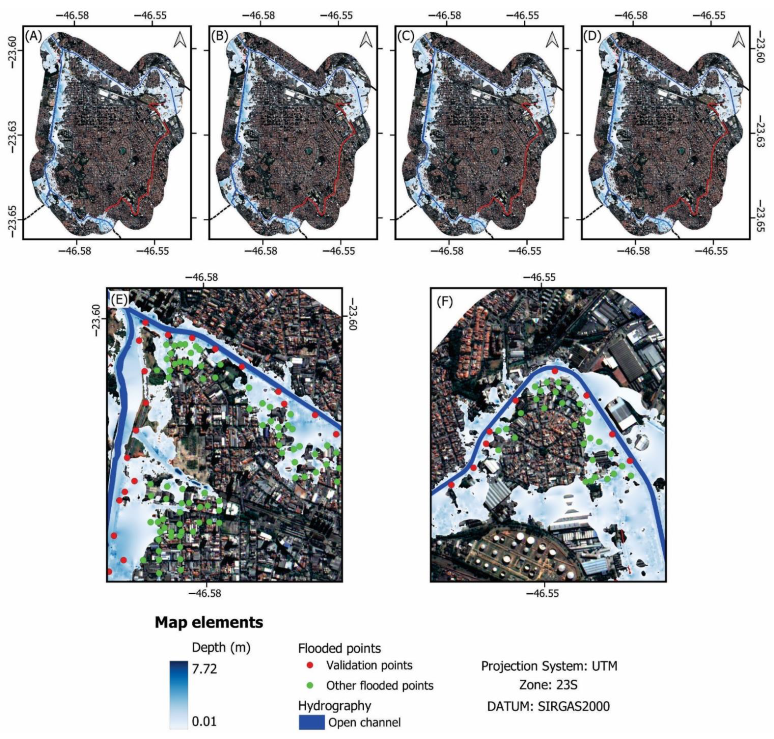
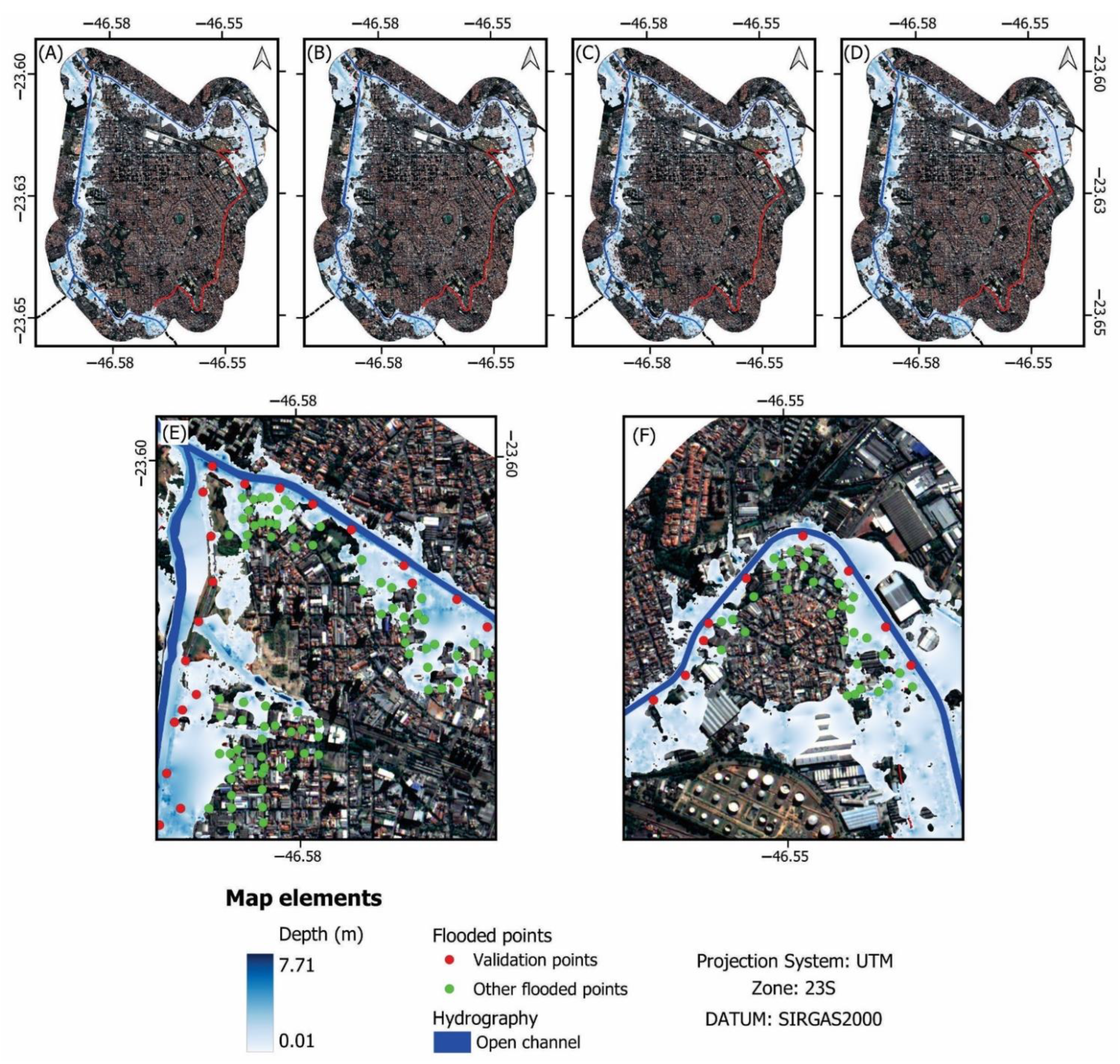
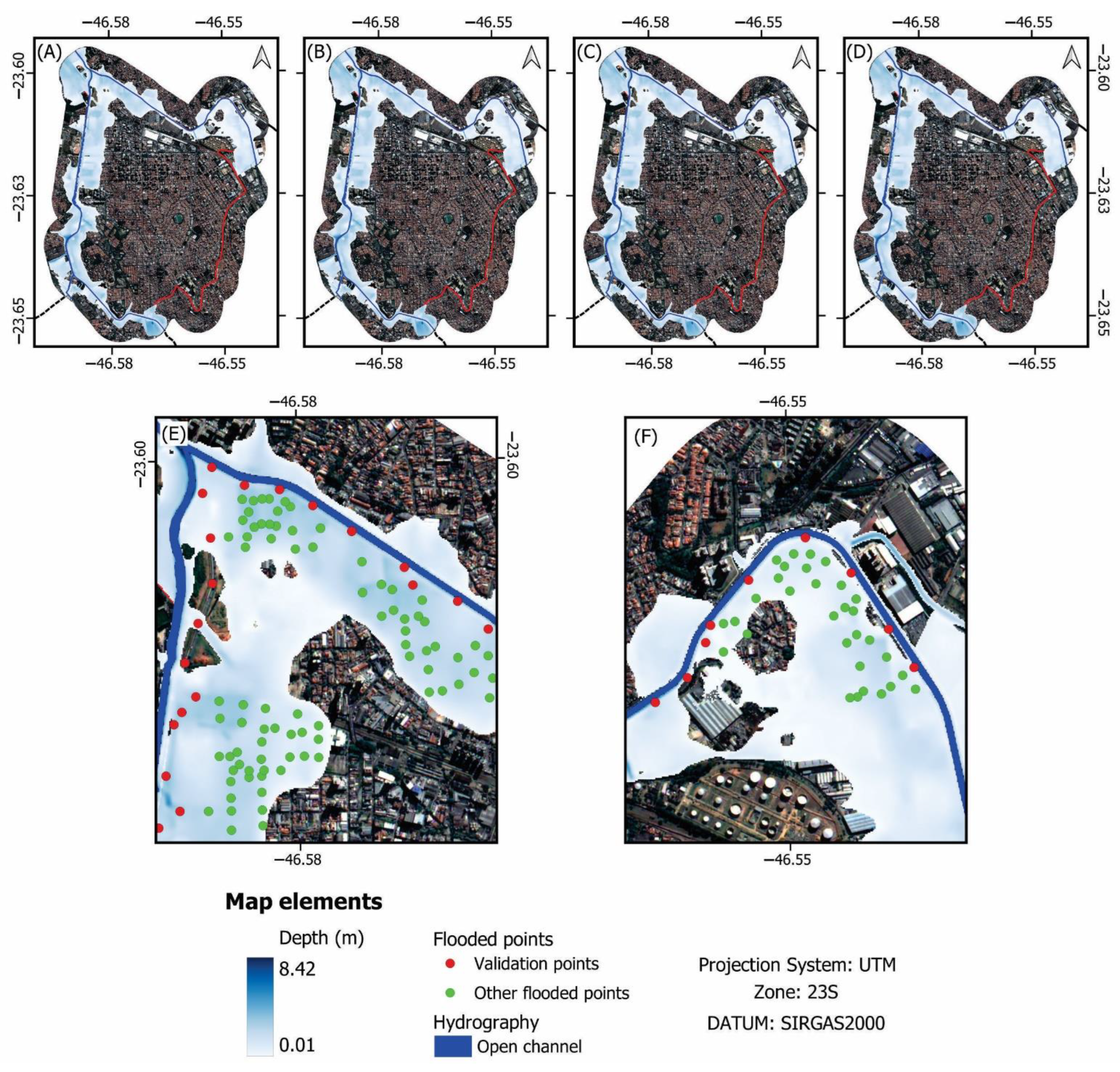
The HEC-RAS simulations for the return period of 79 years with the four computing intervals (1, 15, 30, and 60 s) for three different scenarios (EMPLASA DTM, finer DTM, and finer DTM with refined channel mesh) are shown in Figure 6, Figure 7 and Figure 8. It is important to highlight that only water depth outside the stream channels is shown (water depth inside the channels is excluded for visualization purposes). Enlarged maps of the simulation results are presented in the Supplementary Material (Figures S1–S3).
With respect to the HEC-RAS simulations with the finer DTM (0.50 m) (Figure 6), the simulations with the four computing intervals (1, 15, 30, and 60 s) provide the same minimum and maximum depth, which are between 0.01 and 7.72. The flood spots are quite similar in the four scenarios. However, these simulations did not encompass all reported flooded points by the civil defense and the citizens. Overall, 103 out of 286 flooded points were not simulated and they are concentrated especially in the western and northeastern regions of the city as shown in Figure 6E,F.
As for the HEC-RAS simulations with the finer DTM (0.50 m) with refined channel mesh (Figure 7), the simulations with the four different computing intervals (1, 15, 30, and 60 s) provide the same minimum and maximum depth, ranging from 0.01 to 7.71 m. Despite the difference in the stream channel mesh between the two finer DTMs, the flooded areas are quite similar in the flooding maps produced by both DTMs (Figure 6 and Figure 7). As a result, the simulations generated with the finer DTMs with refined channel mesh produced the same amount of omitted flooded points (103 points in total, mainly in the western and northeastern regions—see Figure 7E,F).
Considering the HEC-RAS simulations with the EMPLASA DTM (Figure 8), the simulations with the four computing intervals (1, 15, 30 and 60 s) show the same minimum and maximum depth of 0.01 and 8.42 m. From all 286 reported flooded points reported by the civil defense and the citizens, only 8 points were not mapped in all 4 simulations. However, some other areas within São Caetano do Sul were mapped in all four simulations, but they were not registered by the authorities (see Figure 8E,F).
Descriptive statistics of the residuals between the 82 validation points and their corresponding points in the HEC-RAS simulations are presented in Table 2, Table 3 and Table 4. Considering the finer DTM, the residuals means range from 0.805 to 0.808 m, while the standard deviation of the four simulations is 1.215 m. The minimum and maximum residual values vary from −1.552 to 3.364 m. A total of 5 out of 82 validation points were not simulated in the 4 simulations. The simulation with the computing interval of 1 s lasted 2 h, 40 min, and 30 s. On the other hand, the simulation with the computing interval of 60 s was performed in 16 min and 58 s (Table 2). The simulation with the computing interval of 60 s was 89.42% faster than the simulation with the computing interval of 1 s.
The residuals between the validation points and their corresponding points in the HEC-RAS simulation with the finer DTM (0.50 m) with refined channel mesh present means between 0.809 and 0.813 m and a standard deviation of 1.210 m (for all the four simulations). A sum of 5 out of 82 validation points were not simulated in the 4 simulations. The simulation with the computing interval of 1 s was executed in 21 h, 08 min, and 20 s. On the other hand, the simulation with the computing interval of 60 s was performed in 50 min and 59 s (Table 3). The simulation with the computing interval of 60 s was 95.98% faster than the simulation with the computing interval of 1 s.
Considering the HEC-RAS simulations with the EMPLASA DTM, the four simulations presented similar results. The means range from 0.591 to 0.596 m. The standard deviations lie between 0.964 and 0.966 m. The minimum and maximum residual values are −1.575 and 2.917 m, respectively. Only 3 out of 82 validation points were not simulated in the 4 simulations. Finally, it is essential to address that these four simulations related to the EMPLASA DTM, like the previous set of simulations associated with the finer DTM with refined mesh, present a meaningful difference in their processing times. The simulation with the computing interval of 1 s was performed in 3 h, 13 min, and 51 s, while the simulation with the computing interval of 60 s was performed in 19 min and 46 s (Table 4). The simulation with the computing interval of 60 s was 89.80% faster than the simulation with the computing interval of 1 s.

4. Discussion

The floods simulation highlights significant overflows of the watercourse on its banks. The flood magnitudes obtained with the different DTMs indicate that the water can inundate several areas around the water courses, including streets and even buildings. The results of the simulations make it possible to describe the severity of such extreme event in terms of spatial extension since they allow a very detailed mapping of the flood zones. Additionally, it is possible to observe that certain stretches of the streams are more prone to flooding due to the difference in relief. It was also observed that the extent of the flood and the water depths are much higher downstream than upstream. For the simulations with the 3 DTMs, it is important to highlight that all maximum depths are in the stream channels located around the confluence of Tamanduateí River and Meninos Brook (northwestern region of the study area).
Simulations with the finer DTM and the finer DTM with refined channel mesh show similar flooded spots in all four computing intervals. The results also indicate that finer grid sizes (0.50 m) are not impacted by different computing intervals between 1 s and 60 s. Furthermore, even channel mesh refinement seems to not interfere in such simulations. However, computational time should be considered since they present significant difference (from over 21 h up to 17 min).
The simulations with the EMPLASA DTM (spatial resolution of 5 m) present the flood maps with the highest coverage of the flooded points, i.e., 278 points out of a total of 286 points were mapped within the shortest computation time. However, there are still some simulated flood spots that were not observed during the extreme flood event [35], especially in the western and northwestern regions.
The EMPLASA DTM was originally derived from orthophotos with 0.45 m of spatial resolution and refined by IBGE topographic charts, using IKONOS-2 imagery as ancillary data [50,51]. It was generated with 1 m of spatial resolution and was rendered available for public use with a downgraded resolution of 5 m.
The DTM generated from the stereo-pair of WV-2 images has a nominal resolution of 0.5 m. Orbital imagery-derived DTMs tend to generate artifacts since one image of the pair is acquired with a given off-nadir angle, and the other image, in its turn, with a different viewing angle. In addition to that, each GCP introduced for generating orbital DTMs brings along an associated noise, which greatly amplifies the errors. In sum, the spatial resolution is not directly related to the DTM accuracy [52]. In the case of the EMPLASA DTM, its native data are much more accurate than the WV-2-derived DTM. And even though downsampled to 5 m, this DTM still preserves its planialtimetric quality. This explains the achievement of better simulation results when using the EMPLASA DTM, with a few omission errors (eight points) and an elevated accuracy (97.20%). This demonstrates that DTMs with high accuracy (and not necessarily with very high spatial resolution) are crucial for obtaining better flood estimations [53,54,55].
This flood event, having taken place on 10 March 2019, crossed the boundary of São Caetano do Sul and hit the municipalities of São Paulo, Santo André, and São Bernardo do Campo. However, since there is no record of flooded points in the database of the civil defenses for such municipalities, it is not possible to validate these simulated floods with HEC-RAS simulations.

5. Conclusions

In this work, we focused on comparing the influence of the spatial resolution of DTM in flood simulation. To do so, we used two DTMs, with spatial resolutions of 5 and 0.50 m (EMPLASA DTM and finer DTM, respectively) applied in a case study in São Caetano do Sul, São Paulo, Brazil. An extreme event was analyzed. The 2D HEC-RAS simulations were performed within three different scenarios simulated on four computing intervals (1, 15, 30, and 60 s). The scenarios were the following (i): the EMPLASA DTM with a mesh size of 5 m; (ii) the finer DTM with a mesh size of 5 m; and (iii) the finer DTM with a mesh size of 5 m in the dry areas and 1 m in the stream channels (using the refinement tool).
The simulations with the EMPLASA DTM (spatial resolution of 5 m) presented the flood maps with the largest coverage of the flooded points (278 points out of 286—97.20%), within the shortest computation times. However, they mapped flood spots that were not observed by the civil defense nor the citizens during the extreme flood event. In addition, we highlight that a DTM with a finer spatial resolution (<0.50 m) derived from spatial images may not produce the best flood simulation compared to a DTM with a spatial resolution of 5 m derived from orthoimages. This demonstrates that highly accurate DTMs, relying on high quality native data, are essential for achieving successful results.
Unlike previous works reported in the literature, our experiment dealt with a real case study, coping with rainfall data, and innovatively provided statistical validation of the obtained results based on field data. According to our results, HEC-RAS proved to be a powerful tool in the identification of areas susceptible to urban flooding. The results should be handled by local decision-makers in order to prevent and mitigate the effects of extreme flooding such as the one occurred on 10 March 2019. The identification of flood-prone areas can help in the management before, during, and after such events, and the availability of such simulations supports timely decisions targeted to tackle the adverse material impacts of these phenomena as well as to protect and save people directly and indirectly affected by them.

Supplementary Materials

The following supporting information can be downloaded at: https://www.mdpi.com/article/10.3390/w15061127/s1. Supplementary Figure S1. Flood maps generated in HEC-RAS using the finer DTM (0.50 cm). (A) represents the simulation with computing interval of 1 s; (B) computing interval of 15 s; (C) computing interval of 30 s; (D) computing interval of 60 s; Supplementary Figure S2. Flood maps generated in HEC-RAS using the finer DTM with refined channel mesh (0.50 cm). (A) represents the simulation with computing interval of 1 s; (B) computing interval of 15 s; (C) computing interval of 30 s; (D) computing interval of 60 s; Supplementary Figure S3. Flood maps generated in HEC-RAS using the EMPLASA DTM (5 m). (A) represents the simulation with computing interval of 1 s; (B) computing interval of 15 s; (C) computing interval of 30 s; (D) computing interval of 60 s; Supplementary Figure S4. Hydrograph of the flow rate provided by Stream Gauge Station 279 on 10 March 2019.

Author Contributions

Conceptualization, E.V.E.-S. and C.M.d.A.; methodology, E.V.E.-S., C.M.d.A. and R.C.D.d.P.; software, E.V.E.-S., M.R.F., C.M.d.A., C.G.d.O. and R.C.D.d.P.; validation, E.V.E.-S.; formal analysis, E.V.E.-S. and C.M.d.A.; investigation, E.V.E.-S.; database, E.V.E.-S., I.B. and K.L.d.R.F.; data curation, E.V.E.-S.; writing—original draft preparation, E.V.E.-S.; writing—review and editing, E.V.E.-S., C.M.d.A., G.B.L.d.S., M.R.F. and R.C.D.d.P.; visualization, E.V.E.-S. and C.M.d.A.; supervision, C.M.d.A. and G.B.L.d.S.; project administration, E.V.E.-S. and C.M.d.A.; funding acquisition, E.V.E.-S. and C.M.d.A. All authors have read and agreed to the published version of the manuscript.

Funding

This study is funded by the São Paulo Research Foundation (FAPESP), grants 2021/11435-4 (E.V.E.S.) and 2020/09215-3 (C.M.d.A.), by the Brazilian National Council for Scientific and Technological Development CNPq, through grant N° 311324/2021-5 (C.M.d.A.); the Brazilian Coordination for the Upgrade of Graduate Personnel CAPES—Finance Code 001 (E.V.E.S.); and the Brazilian Space Agency—AEB (C.M.d.A.).

Data Availability Statement

Data of Stream Gauge Station 279 (code 1000610) can be downloaded at http://sibh.daee.sp.gov.br/nivel (accessed on 10 December 2022).

Acknowledgments

The authors of this work acknowledge the valuable support provided by: (i) the Civil Defense of São Caetano do Sul for sharing the data on flooding points of the analyzed event; (ii) the Water, Sewage and Environmental Sanitation System (Sistema de Água, Esgoto e Saneamento Ambiental—SAESA), in the person of Vitória Garcia, for her support in the development of this work; (iii) the Hydraulic Technological Center Foundation (Fundação Centro Tecnológico de Hidráulica—FCTH), represented by Flavio Conde, for sharing the data on rainfall, flow, and water level quotas in the study area; and (iv) the Geographical and Cartographic Institute (Instituto Geográfico e Cartográfico—IGC) of São Paulo for providing the DTM with 5 m of spatial resolution. E.V.E.S. thanks William Lehman (USACE), Brennan Beam (USACE), Cameron Ackerman (USACE), and Chris Goodell (Kleinschmidt Associates) for the technical support in the operation of HEC-RAS.

Conflicts of Interest

The authors declare no conflict of interest.

References

  1. United Nations (UN). World Population Prospects 2022. Summary of Results; United Nations (UN): New York, NY, USA, 2022.
  2. United Nations Office for Disaster Risk Reduction (UNDRR). Global Assessment Report on Disaster Risk Reduction 2019; United Nations Office for Disaster Risk Reduction (UNDRR): Geneva, Switzerland, 2019. [Google Scholar]
  3. United Nations (UN). World Urbanization Prospects: The 2018 Revision; United Nations, Department of Economic and Social Affairs, Population Division, Eds.; United Nations (UN): New York, NY, USA, 2019; ISBN 9211483190.
  4. Angel, S.; Parent, J.; Civco, D.L.; Blei, A.; Potere, D. The dimensions of global urban expansion: Estimates and projections for all countries 2000–2050. Prog. Plan. 2011, 75, 53–107. [Google Scholar] [CrossRef]
  5. Angel, S.; Parent, J.; Civco, D.L.; Blei, A.M. Atlas of Urban Expansion—The 2016 Edition Volum 1: Areas and Densities; NYU Urban Expansion Program at New York University, UN-Habitat, and the Lincoln Institute of Land Policy: New York, NY, USA, 2016; ISBN 978-1-55844-243-6. Available online: https://www.lincolninst.edu/sites/default/files/pubfiles/atlas-of-urban-expansion-2016-volume-1-full.pdf (accessed on 15 November 2022).
  6. Hardoy, J.E.; Mitlin, D.; Satterthwaite, D. Environmental Problems in an Urbanizing World: Finding Solutions for Cities in Africa, Asia and Latin America, 2nd ed.; Routledge: London, UK, 2013; ISBN 9781853837197. [Google Scholar]
  7. Grimm, N.B.; Faeth, S.H.; Golubiewski, N.E.; Redman, C.L.; Wu, J.; Bai, X.; Briggs, J.M. Global change and the ecology of cities. Science 2008, 319, 756–760. [Google Scholar] [CrossRef] [PubMed] [Green Version]
  8. Faulkner, S. Urbanization impacts on the structure and function of forested wetlands. Urban Ecosyst. 2004, 7, 89–106. [Google Scholar] [CrossRef]
  9. Semadeni-Davies, A.; Hernebring, C.; Svensson, G.; Gustafsson, L.-G. The impacts of climate change and urbanisation on drainage in helsingborg, sweden: Combined sewer system. J. Hydrol. 2008, 350, 100–113. [Google Scholar] [CrossRef]
  10. White, M.D.; Greer, K.A. The effects of watershed urbanization on the stream hydrology and riparian vegetation of los peñasquitos creek, California. Landsc. Urban Plan. 2006, 74, 125–138. [Google Scholar] [CrossRef]
  11. Grabs, W.; Tyagi, A.C.; Hyodo, M. Integrated flood management. Water Sci. Technol. 2007, 56, 97–103. [Google Scholar] [CrossRef] [PubMed]
  12. World Meteorological Organization (WMO). Atlas of Mortality and Economic Losses from Weather, Climate and Water Extremes (1970–2019); WMO-No. 12; World Meteorological Organization: Geneva, Switzerland, 2021; ISBN 9789263112675. [Google Scholar]
  13. Centre for Research on the Epidemiology of Disasters (CRED). Disasters in Numbers. Available online: https://cred.be/sites/default/files/2021_EMDAT_report.pdf (accessed on 23 January 2023).
  14. Emilsson, T.; Sang, Å.O. Impacts of Climate Change on Urban Areas and Nature-Based Solutions for Adaptation. In Nature-Based Solutions to Climate Change Adaptation in Urban Areas; Kabisch, N., Korn, H., Stadler, J., Bonn, A., Eds.; Theory and Practice of Urban Sustainability Transitions; Springer International Publishing: Cham, Switzerland, 2017; pp. 15–27. ISBN 978-3-319-53750-4. [Google Scholar]
  15. Center for Studies and Research in Engineering and Civil Defense (CEPED) Atlas Brasileiro de Desastres Naturais: 1991 A 2012, 2nd ed.; Universidade Federal de Santa Catarina: Florianópolis, Brazil, 2013.
  16. Sprissler, T. Flood Risk in Brazil: Prevention, Adaptation and Insurance; Chennell, J., Heard, R., Eds.; Swiss Re: Zurich, Switzerland, 2011. [Google Scholar]
  17. Integrated Disaster Information System (Sistema Integrado de Informações sobre Desastres—S2iD). Management Report—Reported Damages (Relatório Gerencial—Danos Informados). 2023. Available online: https://s2id.mi.gov.br/ (accessed on 15 January 2023).
  18. Jha, A.K.; Bloch, R.; Lamond, J. Cities and Flooding: A Guide to Integrated Urban Flood Risk Management for the 21st Century; The World Bank: Washington, DC, USA, 2012; ISBN 978-0-8213-8866-2. [Google Scholar]
  19. Rosenzweig, B.R.; Herreros Cantis, P.; Kim, Y.; Cohn, A.; Grove, K.; Brock, J.; Yesuf, J.; Mistry, P.; Welty, C.; McPhearson, T.; et al. The value of urban flood modeling. Earths Future 2021, 9, 9. [Google Scholar] [CrossRef]
  20. Neal, J.C.; Bates, P.D.; Fewtrell, T.J.; di Baldassarre, G. Urban Flood Modelling. In Floods in a Changing Climate: Inundation Modelling; Cambridge University Press: Cambridge, UK, 2012; pp. 69–77. [Google Scholar]
  21. Teng, J.; Jakeman, A.J.; Vaze, J.; Croke, B.F.W.; Dutta, D.; Kim, S. Flood inundation modelling: A review of methods, recent advances and uncertainty analysis. Environ. Model. Softw. 2017, 90, 201–216. [Google Scholar] [CrossRef]
  22. Salvadore, E.; Bronders, J.; Batelaan, O. Hydrological modelling of urbanized catchments: A review and future directions. J. Hydrol. 2015, 529, 62–81. [Google Scholar] [CrossRef]
  23. Rangari, V.A.; Umamahesh, N.V.; Bhatt, C.M. Assessment of inundation risk in urban floods using HEC RAS 2D. Model. Earth Syst. Environ. 2019, 5, 1839–1851. [Google Scholar] [CrossRef]
  24. Tomás, L.R.; Soares, G.G.; Jorge, A.A.S.; Mendes, J.F.; Freitas, V.L.S.; Santos, L.B.L. Flood risk map from hydrological and mobility data: A case study in são paulo (Brazil). Trans. GIS 2022, 26, 2341–2365. [Google Scholar] [CrossRef]
  25. Rennó, C.D.; Nobre, A.D.; Cuartas, L.A.; Soares, J.V.; Hodnett, M.G.; Tomasella, J.; Waterloo, M.J. HAND, a new terrain descriptor using SRTM-DEM: Mapping terra-firme rainforest environments in Amazonia. Remote Sens. Environ. 2008, 112, 3469–3481. [Google Scholar] [CrossRef]
  26. Silva, C.V.F.; Oliveira, C.P.M.; Garcia, J.I.B.; Yazaki, L.F.O.L.; Natale, O.; Brites, A.P.Z. Scenario Evaluation of Alternatives for Flood Control in the Anhangabaú Watershed, Brazil. In Proceedings of the 6th International Conference on Flood Management, São Paulo, Brazil, 16–18 September 2014. [Google Scholar]
  27. Oliveira, C.P.M.; Silva, C.V.F.; Sosnoski, A.S.K.B.; Bozzini, P.L.; Rossi, D.M.; Uemura, S.; Conde, F. Warning System Based on Real-Time Flood Forecasts in São Paulo, Brazil. In Proceedings of the 6th International Conference on Flood Management, São Paulo, Brazil, 16–18 September 2014. [Google Scholar]
  28. Brazilian Institute of Geography and Statistics (IBGE). Cidades e Estados (‘Cities and States’). 2023. Available online: https://www.ibge.gov.br/cidades-e-estados/sp/sao-caetano-do-sul.html (accessed on 20 July 2022).
  29. Brazilian Institute of Geography and Statistics (IBGE). Gross Internal Product of the Brazil’s Municipalities 2018 (‘Produto Interno Bruto Dos Municípios 2018′); IBGE, Ed.; Coordenação de Contas Nacionais: Rio de Janeiro, Brazil, 2020; ISBN 9786587201399. [Google Scholar]
  30. Sustainable Cities Institute (Instituto Cidades Sustentáveis—ICS). Development Index: Brazil (‘Índice de Desenvolvimento Sustentável Das Cidades: Brasil’). 2022. Available online: https://idsc.cidadessustentaveis.org.br/rankings (accessed on 30 January 2023).
  31. Escobar-Silva, E.V.; de Almeida, C.M.; Carvalho, R.M.; de Oliveira, C.G. Generation of a Digital Terrain Model (DTM) in Urban Areas by Means of Very High-Resolution Satellite Images and Combined to a Bathymetric. Bull. Geod. Sci. 2023, in press. [Google Scholar]
  32. Beck, H.E.; Zimmermann, N.E.; McVicar, T.R.; Vergopolan, N.; Berg, A.; Wood, E.F. Present and future Köppen-Geiger climate classification maps at 1-km resolution. Sci. Data 2018, 5, 180214. [Google Scholar] [CrossRef] [Green Version]
  33. CLIMATE-DATA.ORG. Climate São Caetano Do Sul. Available online: https://en.climate-data.org/south-america/brazil/sao-paulo/sao-caetano-do-sul-9603/ (accessed on 31 January 2023).
  34. Moroz-Caccia Gouveia, I.C.; Rodrigues, C. Mudanças Morfológicas e efeitos hidrodinâmicos do processo de urbanização na bacia hidrográfica do rio Tamanduateí—RMSP. GEOUSP Espaço Tempo (Online) 2017, 21, 257. [Google Scholar] [CrossRef] [Green Version]
  35. Civil Defense. Disaster Information Form (Formulário de Informações do Desastre—FIDE). Protocol No. SP-F-3548807-13214-20190310. 2019. Report with restricted access.
  36. G1. Chuva Faz Rua de São Caetano Ficar Com Quase 2 Metros de Água. Available online: https://g1.globo.com/sp/sao-paulo/noticia/2019/03/11/rua-de-sao-caetano-tem-quase-2-metros-de-agua-e-mais-de-20-enchentes-em-35-anos.ghtml (accessed on 23 January 2023).
  37. Seidel, E. Fortes Chuvas Provocam Alagamentos Em São Paulo e Região Metropolitana. Available online: https://mobilidadesampa.com.br/2019/03/fortes-chuvas-provocam-alagamentos-em-sao-paulo-e-regiao-metropolitana/ (accessed on 23 January 2023).
  38. National Water Resources Information System (Sistema Nacional de Informação de Recursos Hídricos—SNIRH). HidroWeb. Available online: https://www.snirh.gov.br/hidroweb/mapa (accessed on 6 July 2022).
  39. Ferraro, D.; Costabile, P.; Costanzo, C.; Petaccia, G.; Macchione, F. A Spectral Analysis Approach for the a Priori Generation of Computational Grids in the 2-D Hydrodynamic-Based Runoff Simulations at a Basin Scale. J. Hydrol. 2020, 582, 124508. [Google Scholar] [CrossRef]
  40. São Paulo Company for Metropolitan Planning (EMPLASA). Digital Terrain Models; São Paulo Company for Metropolitan Planning (EMPLASA): São Paulo, Brazil, 2013; Digital data with restricted access. [Google Scholar]
  41. Brunner, G.W. HEC-RAS: River Analysis System—User’s Manual Version 6.0; US Army Corps of Engineers, Institute for Water Resources, Hydrologic Engineering Center (HEC): Davis, CA, USA, 2021. [Google Scholar]
  42. Xiong, Y. A Dam break analysis using HEC-RAS. J. Water Resour. Prot. 2011, 3, 370–379. [Google Scholar] [CrossRef]
  43. Ahmad, H.F.; Alam, A.; Bhat, M.S.; Ahmad, S. One dimensional steady flow analysis using HECRAS—A case of River Jhelum, Jammu and Kashmir. Eur. Sci. J. 2016, 12, 340. [Google Scholar] [CrossRef]
  44. Quirogaa, V.M.; Kurea, S.; Udoa, K.; Manoa, A. Application of 2D numerical simulation for the analysis of the February 2014 bolivian amazonia flood: Application of the new HEC-RAS version 5. Ribagua 2016, 3, 25–33. [Google Scholar] [CrossRef] [Green Version]
  45. Zainalfikry, M.K.; Ab Ghani, A.; Zakaria, N.A.; Chan, N.W. HEC-RAS One-Dimensional Hydrodynamic Modelling for Recent Major Flood Events in Pahang River. In Proceedings of the AICCE’19: Transforming the Nation for a Sustainable Tomorrow; Springer International Publishing: Cham, Switzerland, 2020; pp. 1099–1115. [Google Scholar]
  46. Garcia, M.; Juan, A.; Bedient, P. Integrating reservoir operations and flood modeling with HEC-RAS 2D. Water 2020, 12, 2259. [Google Scholar] [CrossRef]
  47. Urzică, A.; Mihu-Pintilie, A.; Stoleriu, C.C.; Cîmpianu, C.I.; Huţanu, E.; Pricop, C.I.; Grozavu, A. Using 2D HEC-RAS modeling and embankment dam break scenario for assessing the flood control capacity of a Multi-Reservoir system (NE Romania). Water 2020, 13, 57. [Google Scholar] [CrossRef]
  48. Dasallas, L.; Kim, Y.; An, H. Case study of HEC-RAS 1D–2D coupling simulation: 2002 baeksan flood event in Korea. Water 2019, 11, 2048. [Google Scholar] [CrossRef] [Green Version]
  49. Brunner, G.W. HEC-RAS: River Analysis System Hydraulic Reference Manual; Hydrologic Engineering Center: Davis, CA, USA, 2021. [Google Scholar]
  50. Marques-Carvalho, R.; de Almeida, C.M.; Escobar-Silva, E.V.; de Oliveira Alves, R.B.; Anjos Lacerda, C.S. dos simulation and prediction of urban land use change considering multiple classes and transitions by means of random change allocation algorithms. Remote Sens 2022, 15, 90. [Google Scholar] [CrossRef]
  51. Instituto Geográfico e Cartográfico—IGC. Ortofotos e Modelos Digitais de Superfície—2010/2011. Available online: http://www.igc.sp.gov.br/produtos/listagem_emplasa.html (accessed on 21 February 2023).
  52. American Society for Photogrammetry and Remote Sensing (ASPRS). ASPRS positional accuracy standards for digital geospatial data. Photogramm. Eng. Remote Sens. 2015, 81, 1–26. [Google Scholar] [CrossRef]
  53. Hawker, L.; Bates, P.; Neal, J.; Rougier, J. Perspectives on digital elevation model (dem) simulation for flood modeling in the absence of a high-accuracy open access global dem. Front. Earth Sci. 2018, 6. [Google Scholar] [CrossRef] [Green Version]
  54. Xu, K.; Fang, J.; Fang, Y.; Sun, Q.; Wu, C.; Liu, M. The importance of digital elevation model selection in flood simulation and a proposed method to reduce dem errors: A case study in Shanghai. Int. J. Disaster Risk Sci. 2021, 12, 890–902. [Google Scholar] [CrossRef]
  55. Xing, Y.; Chen, H.; Liang, Q.; Ma, X. Improving the performance of city-scale hydrodynamic flood modelling through a GIS-based DEM Correction Method. Nat. Hazards 2022, 112, 2313–2335. [Google Scholar] [CrossRef]
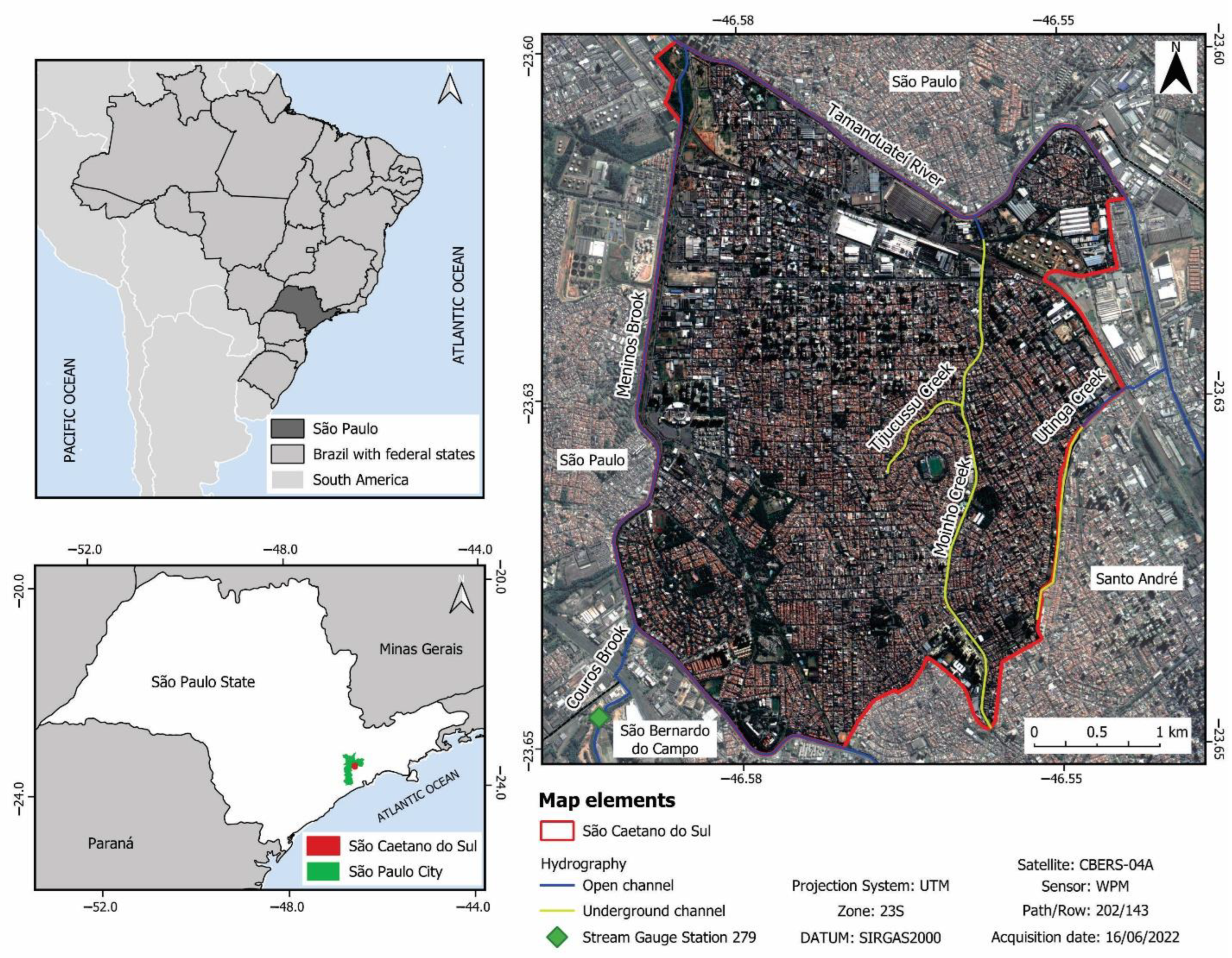
Figure 1. Study area location.
Water 15 01127 g001
Figure 2. Tamanduateí River Watershed location.
Water 15 01127 g002
Figure 3. CBERS-04A satellite image of São Caetano do Sul and its municipal limits (red line) surrounded by a 500 m buffer, indicating flooded points reported by the civil defense of São Caetano do Sul and its citizens on 10 March 2019 (a 79-year return period event). Red points are used for validation since they are reported with estimated water depth.
Water 15 01127 g003
Figure 4. Some photos of the floods on 10 March 2019 in São Caetano do Sul. Source: (A,B) [36]; (C) [37].
Water 15 01127 g004
Figure 5. Methodological flowchart.
Water 15 01127 g005
Figure 6. Flood maps generated in HEC-RAS. (AD) represent the simulations with the computing interval of 1, 15, 30, and 60 s, respectively, with the finer DTM (0.50 m). (E) is a zoom-in of the confluence of Tamanduateí River and Meninos Brook in the northwestern region of the study area. (F) shows a zoom-in of the Tamanduateí River in the northeastern part of the analyzed reach. Red points are used for validation, while the green points represent other flooded points reported by the citizens of São Caetano do Sul. The thick lines in dark blue correspond to the open channels. The different shades of blue in polygonal shape account for the different depths of the flood zones.
Water 15 01127 g006
Figure 7. Flood maps generated in HEC-RAS. (AD) represent the simulations with the computing interval of 1, 15, 30, and 60 s, respectively, with the finer DTM (0.50 m) with refined channel mesh. (E) is a zoom-in of the confluence of Tamanduateí River and Meninos Brook in the northwestern region of the study area. (F) shows a zoom-in of Tamanduateí River in the northeastern part of the analyzed reach. Red points are used for validation, while the green points represent other flooded points reported by the citizens of São Caetano do Sul. The thick lines in dark blue correspond to the open channels. The different shades of blue in polygonal shape account for the different depths of the flood zones.
Water 15 01127 g007
Figure 8. Flood maps generated in HEC-RAS. (AD) represent the simulations with the computing interval of 1, 15, 30, and 60 s, respectively, with the EMPLASA DTM (5 m). (E) is a zoom-in of the confluence of Tamanduateí River and Meninos Brook in the northwestern region of the study area. (F) shows a zoom-in of Tamanduateí River in the northeastern part of the analyzed reach. Red points are used for validation, while the green points represent other flooded points reported by the citizens of São Caetano do Sul. The thick lines in dark blue correspond to the open channels. The different shades of blue in polygonal shape account for the different depths of the flood zones.
Water 15 01127 g008
Table 1. Most relevant flood events in São Caetano do Sul between 2000 and 2022 *.
Year
(Descending Order)
Number of Events Per YearDates of Occurrence
(Day/Month)
2022402/0217/0201/0312/03
2021118/11
2020308/0119/0224/02
2019304/0215/0210/03
2018217/1023/11
2017306/0206/0427/11
2016215/0206/06
2015127/01
2012217/0128/11
2011215/1114/12
2010117/02
2008121/02
2005111/01
2002128/11
2000212/0126/01
Note: * 29 events were found from a search carried out by the authors in databases of newspapers, journals, and the civil defense of São Caetano do Sul considering the period between 2000 and 2022, shown in descending chronological order.
Table 2. Descriptive statistics of the residuals between the 82 validation points and their corresponding points in the HEC-RAS simulation with the finer DTM (0.50 m).
Finer DTMFiner DTMFiner DTMFiner DTM
Computing intervals1 s15 s30 s60 s
Mean (m)0.8050.8060.8060.808
Standard deviation (m)1.2151.2151.2151.215
Range (m)4.9104.9094.9104.913
Minimum (m)–1.552–1.552–1.551–1.549
Maximum (m)3.3573.3583.3593.364
Missing points5555
Computation time (hh:mm:ss)02:40:3000:55:3200:30:2400:16:58
Table 3. Descriptive statistics of the residuals between the 82 validation points and their corresponding points in the HEC-RAS simulation with the finer DTM (0.50 m) with refined channel mesh.
Finer DTM with Refined Channel MeshFiner DTM with Refined Channel MeshFiner DTM with Refined Channel MeshFiner DTM with Refined Channel Mesh
Computing intervals1 s15 s30 s60 s
Mean (m)0.8090.8100.8110.813
Standard deviation (m)1.2101.2101.2101.210
Range (m)5.0385.0385.0395.040
Minimum (m)–1.626–1.625−1.624–1.621
Maximum (m)3.4123.4133.4143.420
Missing points5555
Computation time (hh:mm:ss)21:08:2002:50:3101:37:3900:50:59
Table 4. Descriptive statistics of the residuals between the 82 validation points and their corresponding points in the HEC-RAS simulation with the EMPLASA DTM (5 m).
EMPLASA DTMEMPLASA DTMEMPLASA DTMEMPLASA DTM
Computing intervals1 s15 s30 s60 s
Mean (m)0.5910.5910.5920.596
Standard deviation (m)0.9660.9660.9660.964
Range (m)4.4934.4934.4924.484
Minimum (m)–1.577–1.576–1.575–1.566
Maximum (m)2.9172.9172.9172.917
Missing points3333
Computation time (hh:mm:ss)03:13:5100:50:4600:30:5100:19:46
Disclaimer/Publisher’s Note: The statements, opinions and data contained in all publications are solely those of the individual author(s) and contributor(s) and not of MDPI and/or the editor(s). MDPI and/or the editor(s) disclaim responsibility for any injury to people or property resulting from any ideas, methods, instructions or products referred to in the content.