1. Introduction
Floods in cold climates are caused mainly by snowmelt [
1], and ice jams are responsible for some of the northern rivers’ most severe and recurrent floods [
2]. River ice has a significant impact on nearly 66% of rivers in the Northern Hemisphere [
3]. Ice-jam-induced floods can occur rapidly, posing a risk to public safety, infrastructure, and hydropower generation, as well as causing ecological effects due to the scouring and erosion of the riverbeds [
4,
5,
6].
The freeze-up process in rivers is driven by the cooling of the water, which causes the formation of ice on the surface and along the riverbanks. When the temperature drops below freezing during the winter, this process normally takes place. On the other hand, the break-up process takes place in the spring when the temperature starts to rise, and the ice starts to melt. A number of variables, such as solar radiation, air temperature, and water velocity, influence the break-up process [
7].
In winter months, flow reaches a low value for a period, and it keeps the river frozen at low flow until the spring snowmelt time when the break-up stage begins, and then the flow usually reaches its annual maximum value [
8,
9,
10,
11]. Occasionally, peak flows in large rivers occur in summer or autumn due to rainfall or snowmelt events. Changes in the timing and severity of the break-up event, whether due to relatively abrupt channel regulation or gradual climatic variation, are likely to have significant ecological consequences [
8,
12]. The magnitude of flow and flow-rate characteristics, such as timing, duration, and frequency, are related to the dimensions of aquatic ecosystem components and the number of inhabitants they contain, and this suggests that the natural flow regime is an important factor in aquatic ecosystems [
13,
14]. Flow regimes, defined by the temporal variability of stream flow, are regarded as an affecting variable that controls the biotic interactions and physicochemical characteristics of a riverine habitat at the basin scale, including channel morphology, sediment flux, water quality, and habitat diversity [
14].
Limited studies exist on the timing characteristics of river ice or that focus on analyzing the discharge time series on frozen rivers. For example, one study used the Theil–Sen slope to estimate the trend in the timing and magnitude of floods [
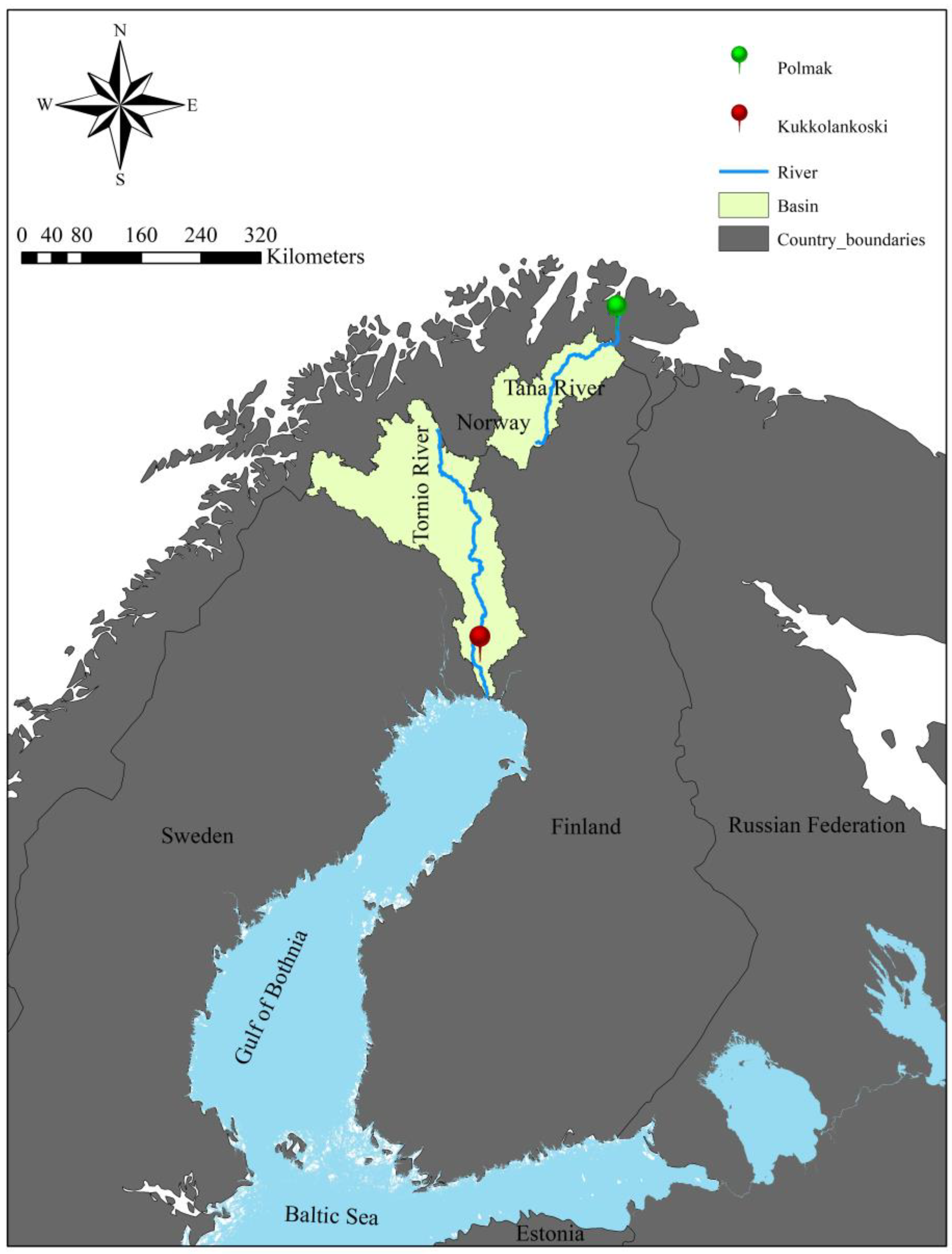
15]. In this study we pursue developing a tool to detect the break-up date (BUD) on each annual daily hydrograph using a simple method that detects the BUD in the transitional period when the discharge starts to rise again in the spring. The RiTiCE (River break-up Timing Characteristics and Extreme flow analyzer) is developed in MATLAB and the objective of this tool is to quantify and detect the BUD and generate novel indices including periods with low flow and examine their characteristics, such as duration, probable shifts through time, and overall flow characteristics, including the average low and high flow in a period of 90 days annually. This study focuses on the duration, shifts, and break-up timings of two unregulated case studies in Finland, i.e., the Tornio and Tana Rivers. Daily discharge data over a period of 100 years in one station on each river are available and are utilized to develop the RiTiCE. The data have been collected from “The Global Runoff Data Centre, 56068 Koblenz, Germany at grdc.bafg.de” and Swedish Meteorological and Hydrological Institute (SMHI). Additionally, we have utilized assimilated MODIS Land Surface Temperature (LST) data to collect daily temperature data after 2002. This study focuses on the events and trends. Therefore, an investigation of the causes is not considered in this research paper due to their strong relationship with several physical and hydrological driving factors for each specific case.
3. Results
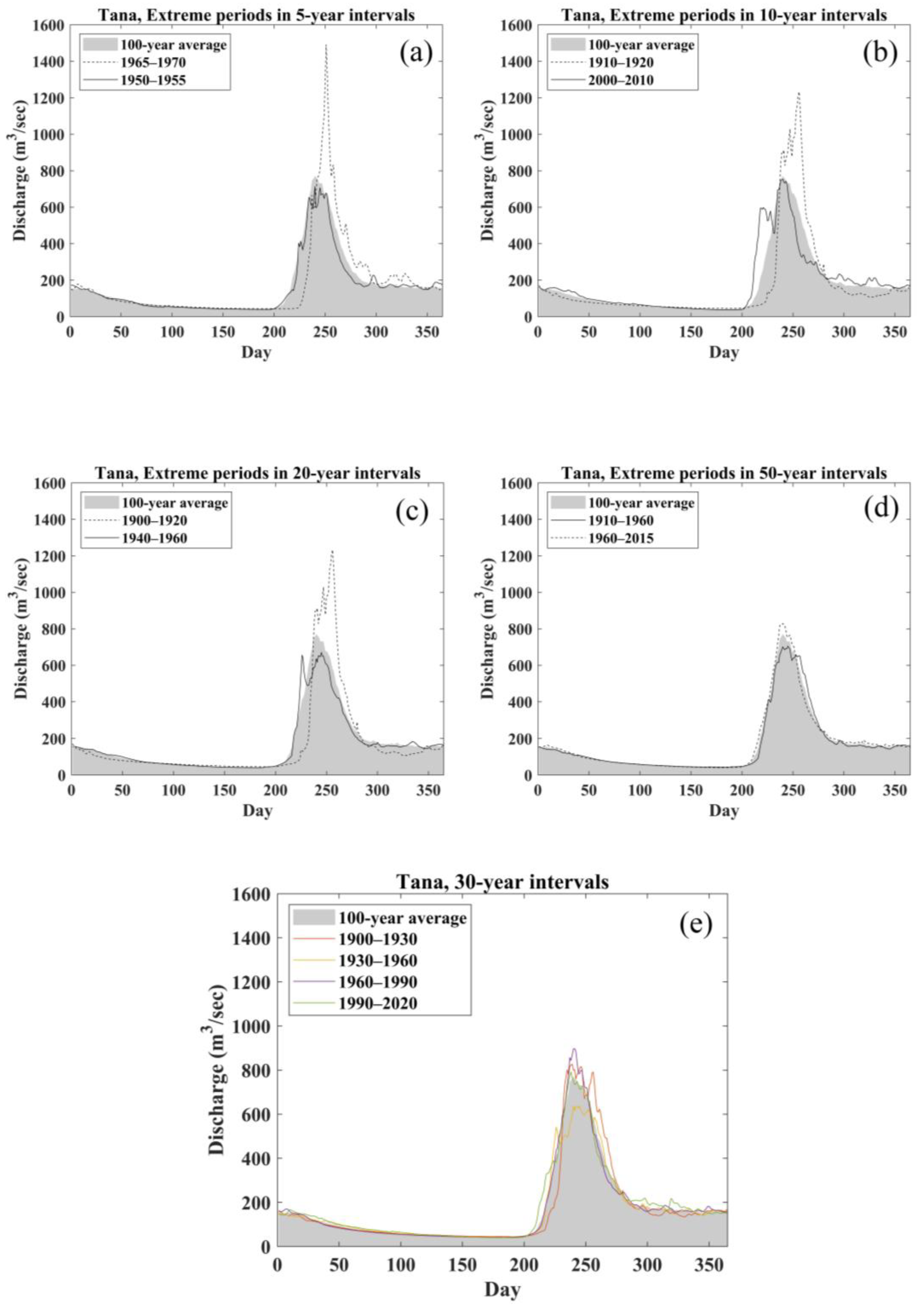
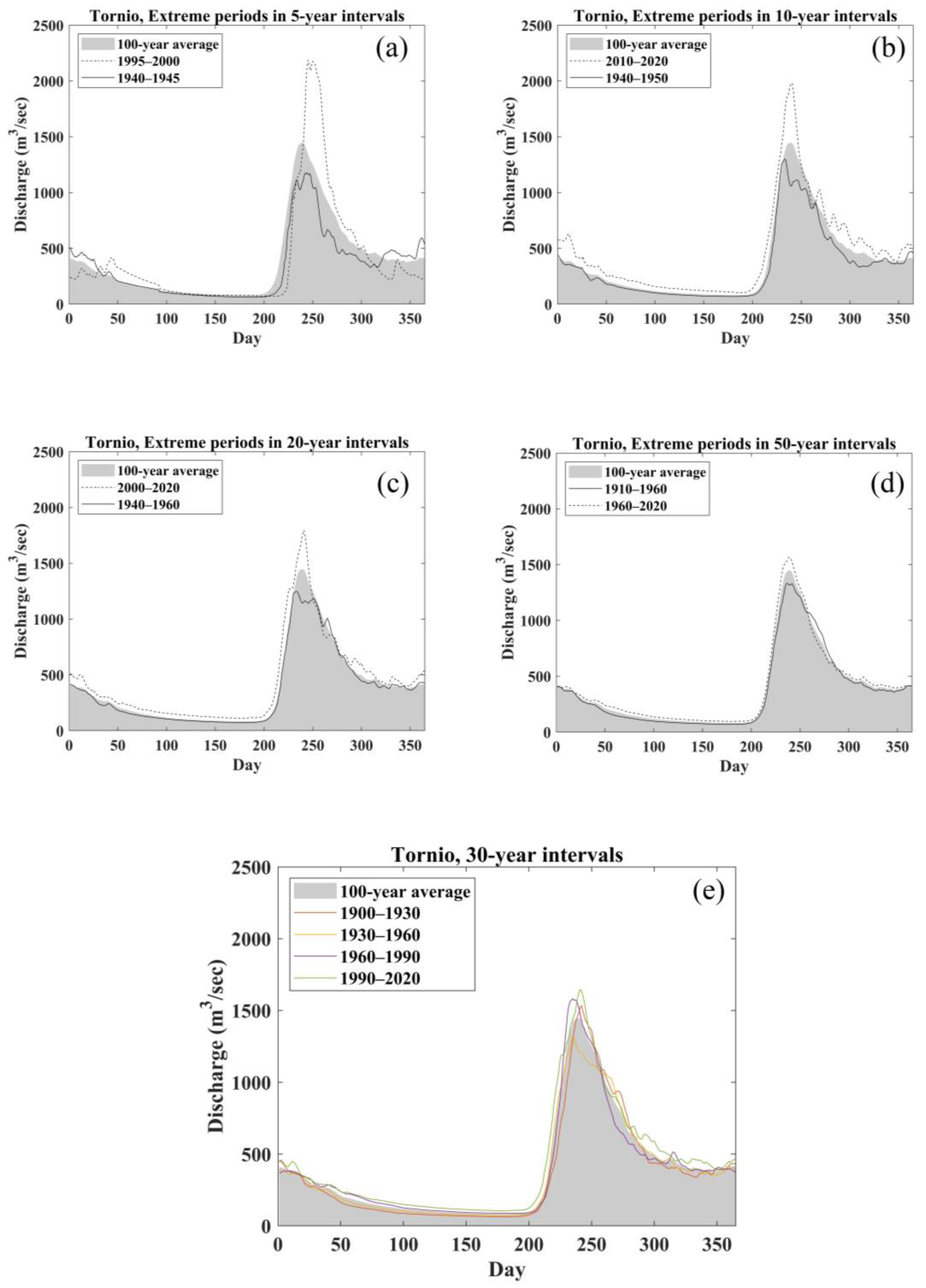
In 5-year intervals, two periods, 1965–1970 and 1950–1955, in the Tana River are extreme discharge periods with the highest and lowest discharge peaks, respectively. In the Tornio River, the highest discharge peak is during 1995–2000, and the lowest discharge peak is observed during 1940–1945 (
Figure 4a and
Figure 5a). In 10-year intervals, the highest and lowest discharge peaks occur in 1911–1920 and 2000–2010, respectively, in the Tana River (
Figure 4b), and in the Tornio River, the highest and lowest discharge peaks occur in 2010–2017 and 1940–1950, respectively (
Figure 5b). The result of the 20-year intervals shows that, in the Tana River, the highest discharge peak extreme period is 1911–1930, and the lowest discharge peak occurs in the 1940–1960 period (
Figure 4c). In the Tornio River, the same extreme periods occur in the 2000–2017 and 1940–1960 periods, respectively (
Figure 5c). For 50-year interval results of the Tana River, the highest discharge peak occurs in the first half (
Figure 4d), although, in the Tornio River, the extreme period with the highest discharge peak occurs in the second half of the period (
Figure 5d). Finally, the datasets are divided into 30-year intervals. The results show that the highest discharge peak is in 1960–1990 and the lowest discharge peak occurs in 1930–1960 in the Tana River. On the other hand, in the Tornio River, the highest and lowest discharge peaks occur in the 1990–2017 and 1930–1960 periods, respectively (
Figure 4e and
Figure 5e).
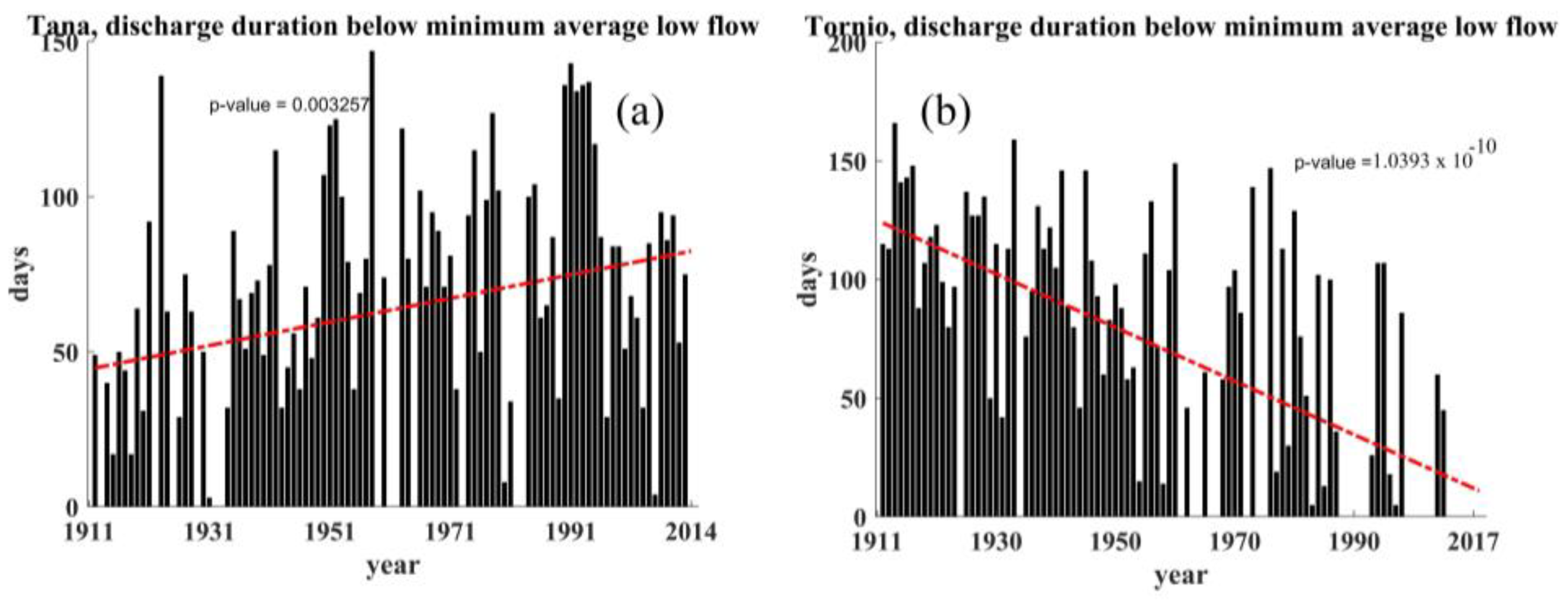
The duration of the period in which the discharge is lower than the minimum 90-day flow in Year365 has been significantly increased from 50–70 days to 100–140 days by a confidence level of 95% in the Tana River (
Figure 6a). In contrast, in the Tornio River, the duration has been significantly decreased by a confidence level of 95%. In the first ten years, the duration is, on average, about 120 days, while the duration in the last ten years is about 50 days (
Figure 6b).
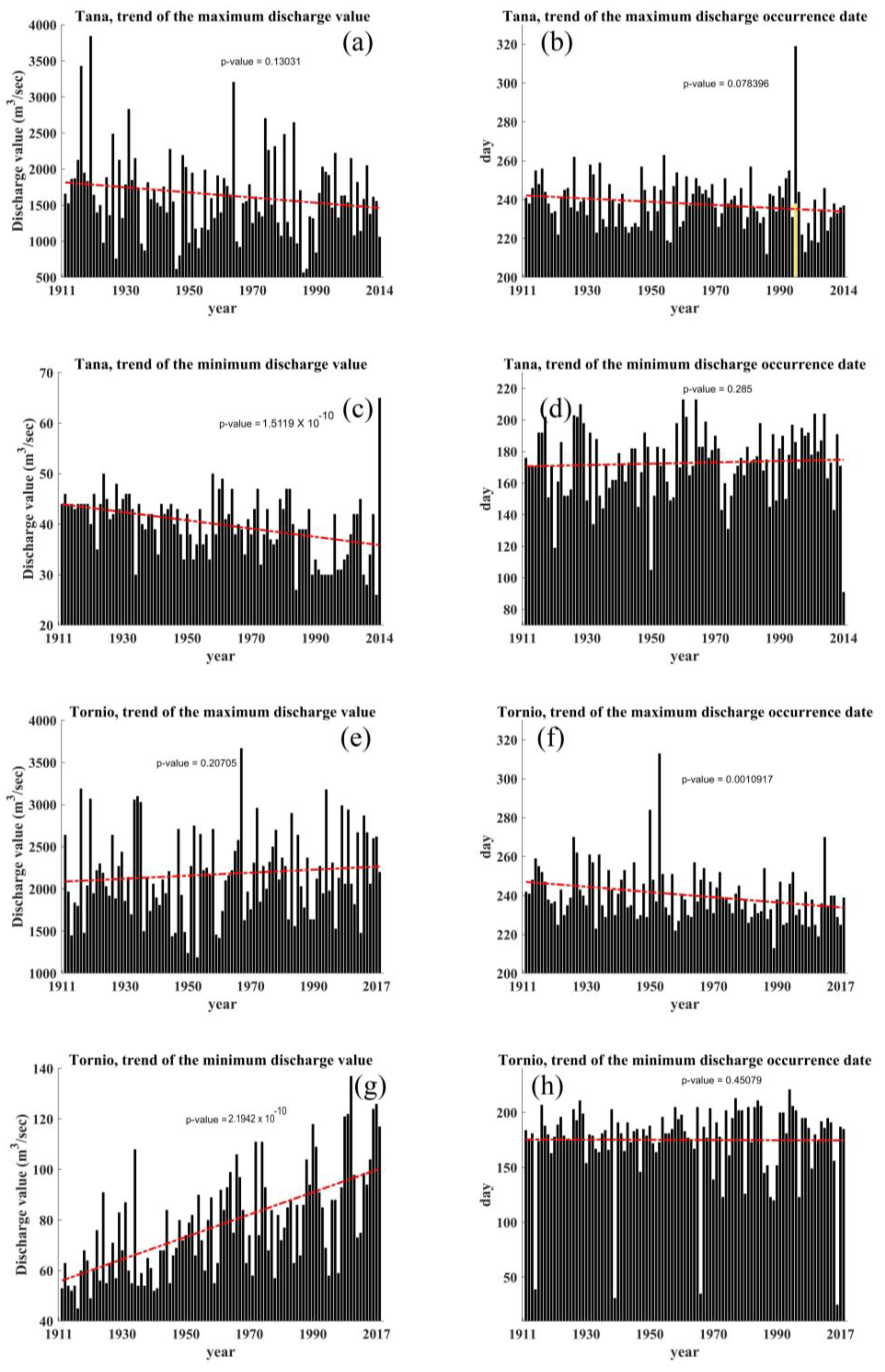
The M–K trend test does not show any significant trend in annual maximum discharge in the Tana River (
Figure 7a). However, as the results show, the maximum discharge value tends to reduce in the latest years and the peaks are smaller than before. The Tornio River does not show any significant change in the annual maximum discharge either (
Figure 7e). The Tana River also experiences a significant reduction in the annual minimum discharge with a confidence level of 95% (
Figure 7c). However, the annual minimum discharge in the Tornio River significantly increases with the same confidence level (
Figure 7g). It appears that the annual maximum discharge in the Tana River may have shifted backwards, but the trend is not significant (
Figure 7b). The same shift takes place in Tornio with a confidence level of 95% (
Figure 7f). The annual minimum discharge occurrence date in both rivers has not changed significantly.
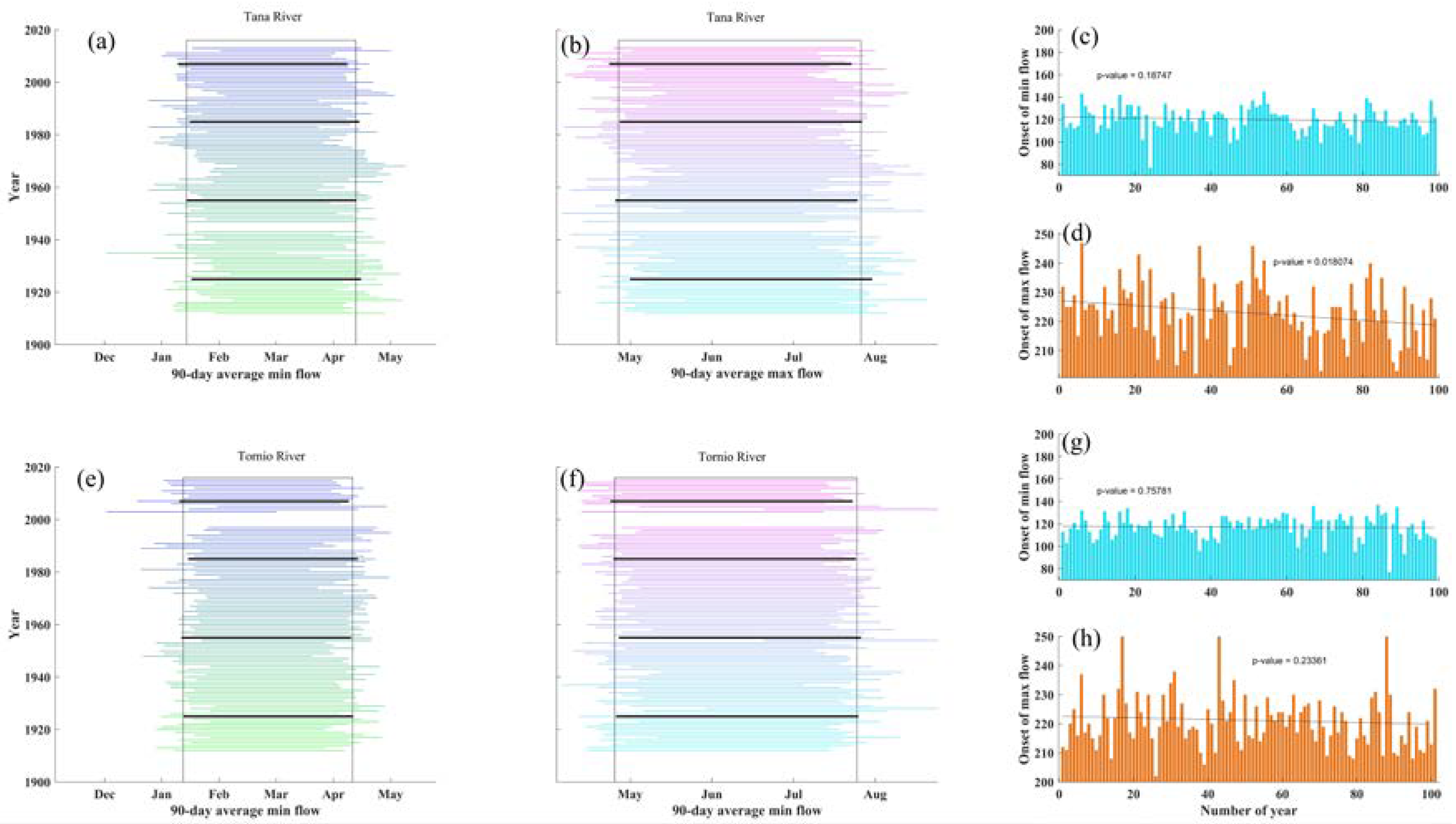
The seasonal extreme mean flow (whether maximum or minimum) in Year365 is shown by the black rectangle in
Figure 8. In the Tana River, the lowest 90-day flow starts in the middle of January and ends in April, over an average of 100 years (
Figure 8a). The highest 90-day flow starts in May and ends before August (
Figure 8b). The same results occurs in the Tornio River for maximum and minimum 90-day flow over an average of 100 years (
Figure 8e,f). Each dataset has been divided into 25-year periods and the results show that, in the Tana River, there has been a shift in the beginning and ending of the maximum and minimum 90-day flow every 25 years (
Figure 8a,b,e,f). More precisely, recent years (1990–2017) have been experiencing more severe shifts in starting and ending dates. In other words, in both rivers, over later years, the minimum 90-day flow tends to occur sooner in January and the maximum 90-day period tends to occur before May. However, in the Tornio River, only the last 25 years reveal the shift; the Tana River shows that the first and second 25 years have shifted to the right (meaning that the minimum and maximum 90-day flows have occurred later than average).
The analyses illustrate that the starting date of the minimum flow in the Tana River varies from the 15th to 100th day from 1 October. However, the results do not show any significant change in the starting date of the minimum 90-day flow. On the other hand, there is a significant backward shift in the starting date of the maximum 90-day flow with a confidence level of 95% (
Figure 8d). The analyses of the Tornio River do not show any significant shifts in either minimum or maximum 90-day flow (
Figure 8g,h).
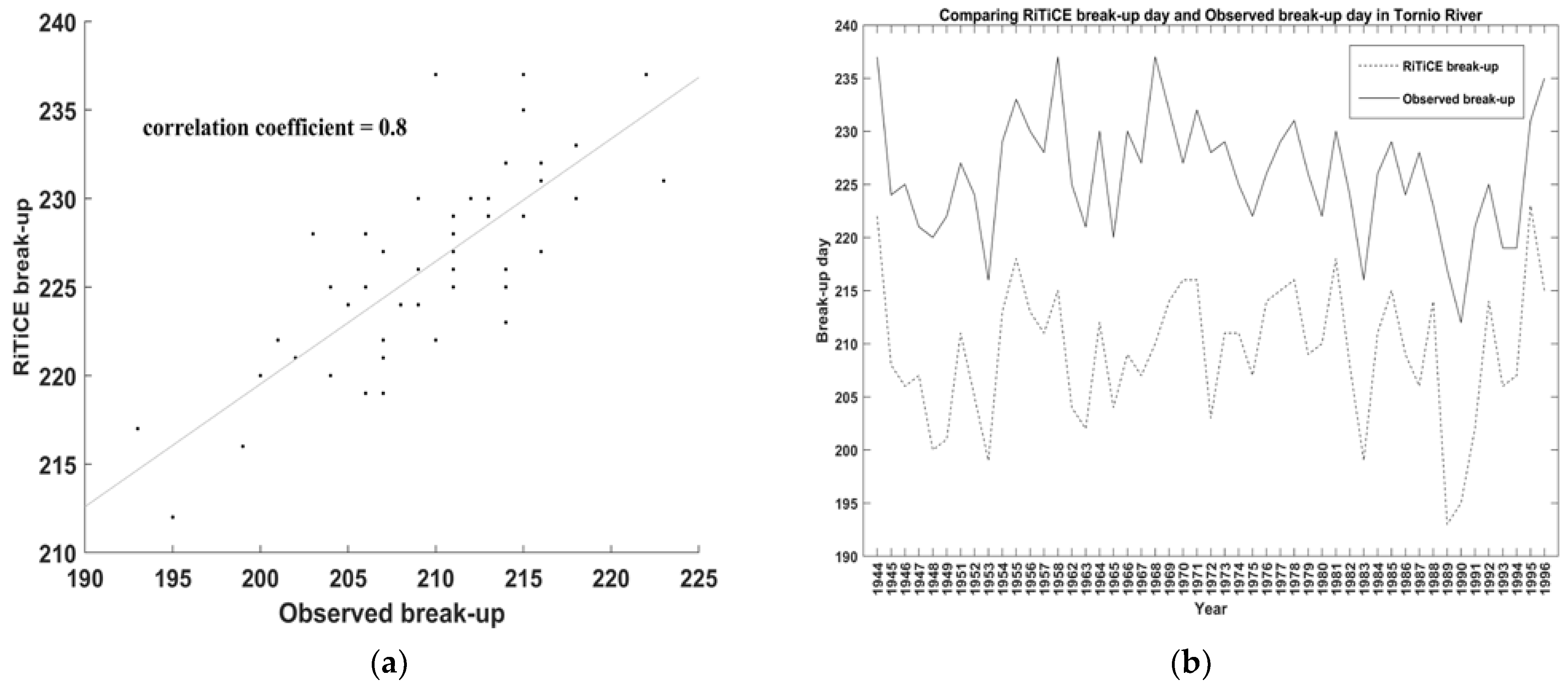
The BUD detection by the RiTiCE is verified by the real observation data on the Tornio River (
Figure 9) for the available period (1944–1996). The results of the comparison between BUDs calculated by the RiTiCE and observed BUDs show a strong correlation of 0.8 (using the Pearson correlation coefficient).
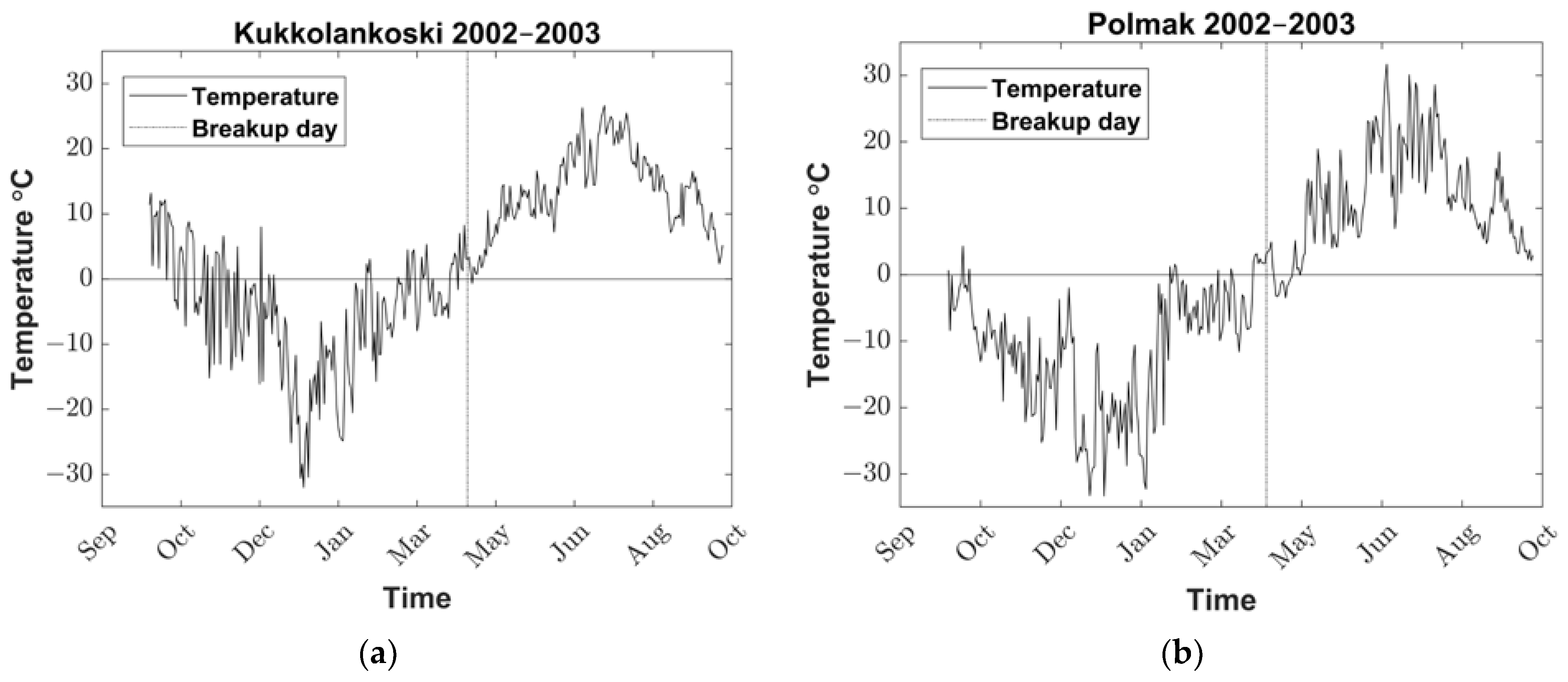
The results of our study show a clear relationship between annual daily temperature and the BUD calculated by the RiTiCE.
Figure 10 illustrates that, as the positive phase of temperature begins, the break-up of the ice also starts to initiate. This supports our hypothesis that temperature plays a significant role in the timing of ice break-up. Detailed results for all years are included in the
Supplementary Materials “Figures S3 and S4” folders.
4. Discussion
The study aims to find solutions for detecting the ice BUD from annual daily hydrographs and verifying the results by observed data. In addition, the study has developed indices to analyze the extreme values, trends, and probable shifts of flow characteristics through time.
It is worth mentioning that the long-term discharge datasets have some gaps. In the Tana River, data from the years 1944–1946, and in the Tornio River, data from the years 1997–2002, are missing. As the intervals are the average daily discharge values for a specific period, the periods that cover the missing data are not comparable to the remaining periods. For instance, in the Tana River, the interval of 20 years would result in two extreme periods for 1911–1930 and 1940–1960, from which the latter is considered the lowest discharge peak among other periods. This could be affected by missing data in that period. On the other hand, while comparing extreme periods in 5-year intervals in the Tornio River, the highest discharge peak belongs to the period 1995–2000, from which 3 years are missing. This leads to some uncertainties regarding the results, especially the intervals at which the extreme periods have been chosen.
The river ice break-up is induced by warm weather, including thermal degradation, initial fracturing, mobility, fragmentation, transport, jamming, and final clearance [
28]. Although some or all these procedures may take place simultaneously to a certain extent, the break-up cycle can be seen as a sequence of distinct phases, such as pre-break-up, onset, driving, and washing [
29]. Onset depends on many factors, including the morphology of the channel. Thus, it is common to see areas that have begun to change phases with areas that have not lost their ice. For different lakes and rivers, the BUD has long been done in Nordic Regions. However, not a certain indicator is found to address the break-up event equally. The main benefit of using the RiTiCE method is that it is based on our specific definition of the river break-up point, which is the point after which the discharge starts to increase in the spring. This method directly addresses our research question and provides a clear answer.
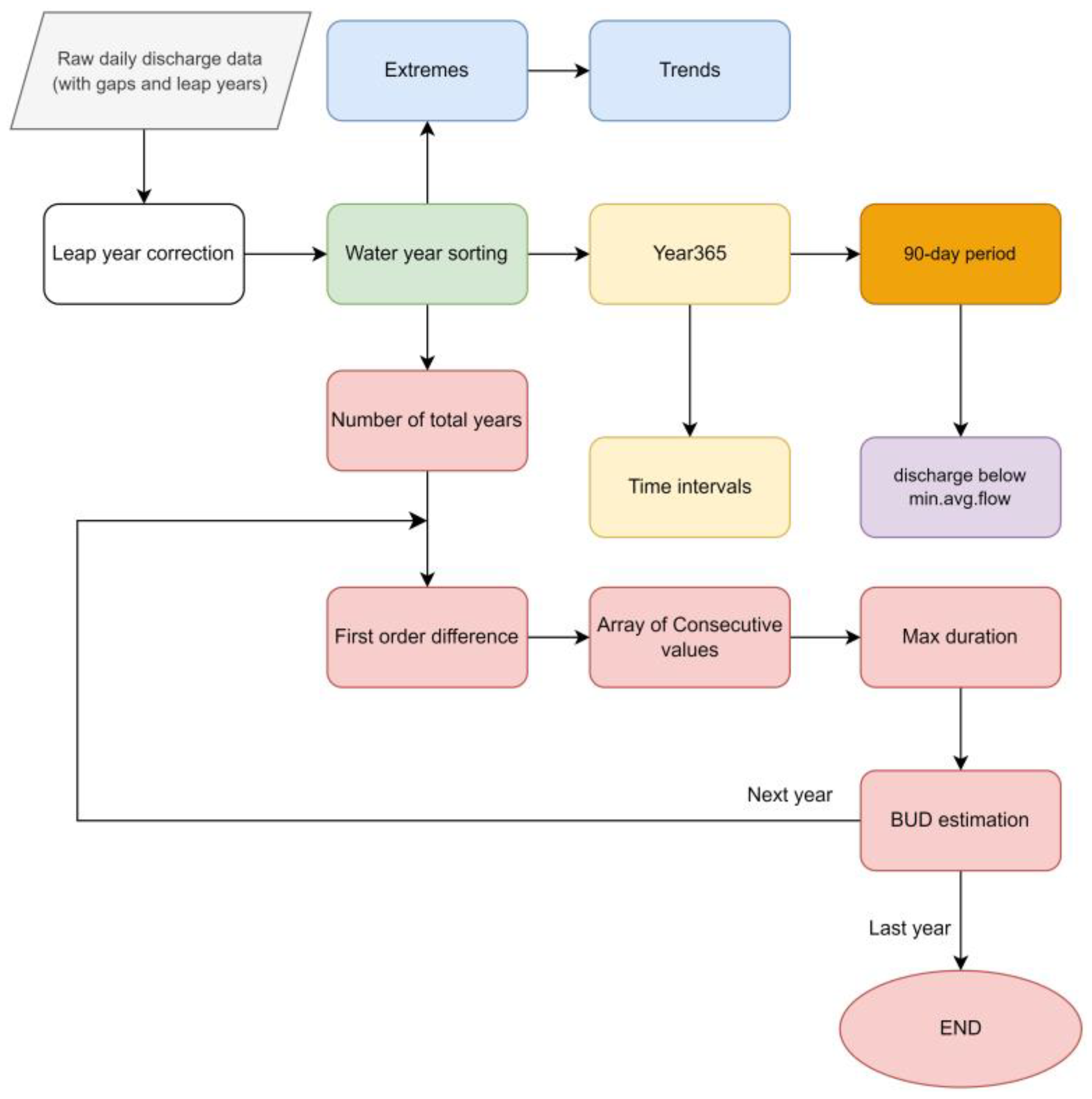
Another benefit of using the RiTiCE is that it is simple and easy to implement, based on a simple first-order difference of the consecutive values, and does not have any assumptions about the underlying distribution of the data. In addition, it also correlates well with the observed data. This suggests that the predictions made by the RiTiCE are closely aligned with the actual observed BUDs. However, it is also important to note that, although there is a significant correlation, on average, the BUDs calculated by the RiTiCE are 16 days before the observed data, owing to different definitions for ice break-up (i.e., raft movement by the Lion’s club vs. onset of discharge increase by the RiTiCE).
The methodology uses absolute maximum and minimum values for the discharge trends. It is assumed that the highest peak belongs to the spring discharge due to the snowmelt. However, in some years, a summer peak discharge is considered an outlier in the results as it is due to precipitation in the summer. In addition, periods below minimum flow correspond well with the results of discharge extremes. As it has been found that the minimum discharge values follow a significantly negative trend in the Tana River, the number of days during which the discharge value is below minimum flow (i.e., metrics from annual 90-day periods) increases significantly. The Tornio River has experienced a significant increment in its minimum discharge over the century, meaning the number of days during which the discharge value is below the minimum flow has decreased significantly.
The number of days in a year where the flow is below the minimum average low flow, of both the Tana and Tornio Rivers, has undergone significant changes, as shown in
Figure 6. However, the trends are opposite in direction. The Tana River (as seen in
Figure 6a) has experienced an increase in the number of days where the flow is below the minimum average low flow, indicating a higher likelihood of minimum flow in recent years. This is supported by the significant decreasing trend in the minimum discharge value of the Tana River, as seen in
Figure 7c.
On the other hand, the Tornio River (
Figure 6b) has experienced a decrease in the number of days where the flow is below the minimum average low flow, meaning that there is a lower chance of minimum flow in recent years. This is confirmed by the significant increasing trend in the minimum discharge value of the Tornio River, as seen in
Figure 7g.
The current study can proceed by researching the reasons for such significant trends in these two stations. Obviously, several climatic factors can drive the river ice phenomena. As rivers react differently to climatic factors, not all models would work on every specific case.
5. Conclusions
River ice, and consequently, ice jam floods, are natural phenomena in cold climate regions. This study developed a tool called RiTiCE to examine the river flow timing characteristics and extreme discharges, along with detecting the break-up date (BUD). Two case studies are located on the Tornio and Tana Rivers on the Finnish borders of Sweden and Norway. The stations provide a century of daily discharge data, which are employed to evaluate the timing, and possible events shifts. Several characteristics have been developed for this purpose, considering Year365 as a metric to highlight the extreme events and corresponding years. From the same perspective on data, the 90-day periods show us that both low and high flows in the two rivers have a negative trend in their occurrence date, meaning the extreme seasonal discharges have tended to occur sooner in recent years. The Tana River does, however, show a negative trend in its annual minimum flow over the century, which contrasts with the Tornio River. The BUD detection by the RiTiCE has been verified through comparison with actual observation data in the Tornio River for 1944–1996. The comparison results demonstrate a strong correlation of 0.8 between the calculated and observed BUDs, indicating that the RiTiCE is an effective method for determining BUDs in this particular river. Finally, it was found that these two rivers have been experiencing a change in the duration of their low-flow periods. The Tana River shows a rise in the duration of its low-flow period, while the opposite is true for the Tornio River.


 ,
, 