
Implications of a Large River Discharge on the Dynamics of a Tide-Dominated Amazonian Estuary

 , ,
, , 
Abstract
1. Introduction
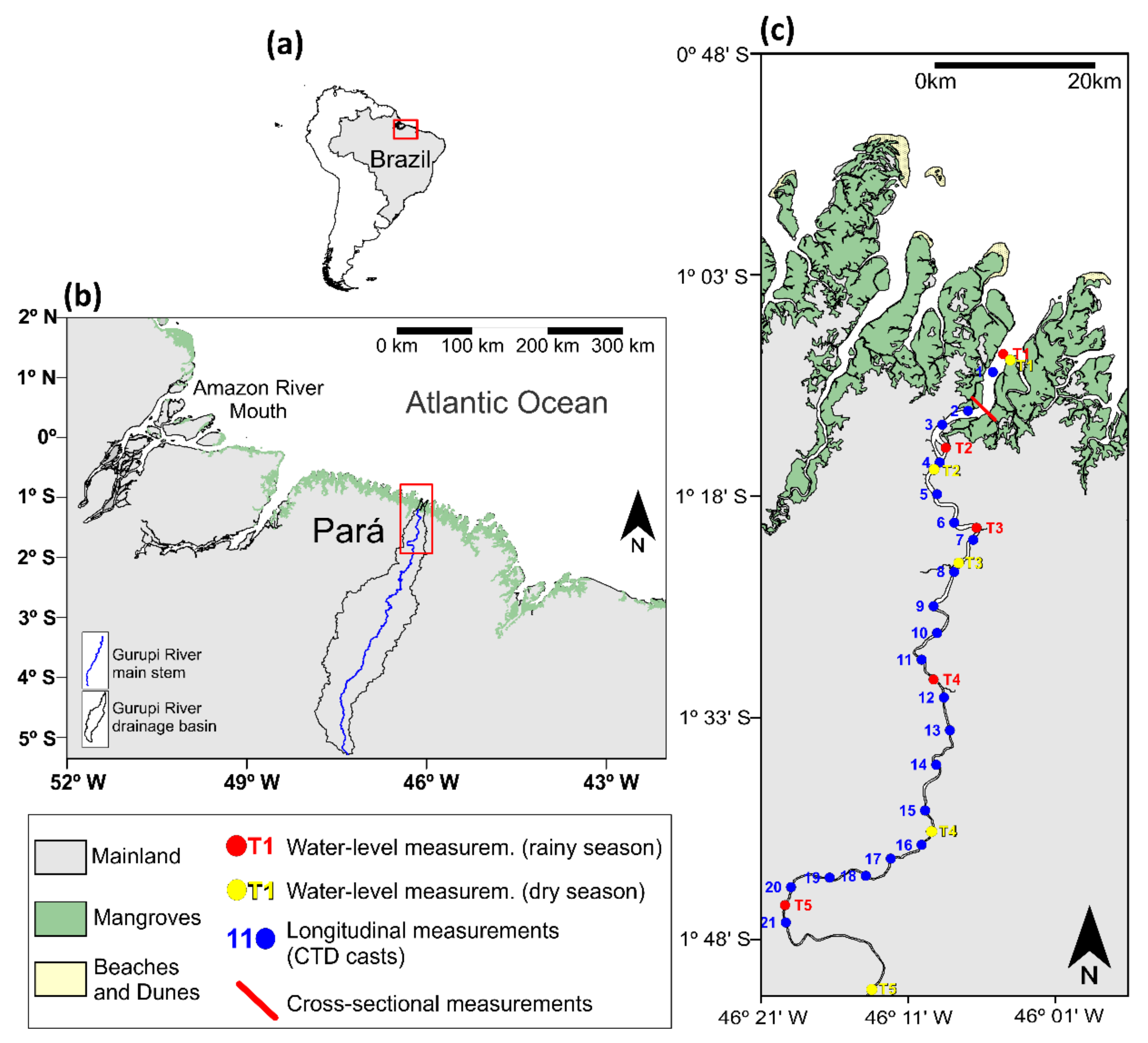
2. Study Area
3. Materials and Methods
3.1. Fixed Instruments
3.2. Boat-Based Longitudinal Surveys
3.3. Boat-Based Transversal Surveys
3.4. Data Processing
3.5. Statistics Analyses
4. Results
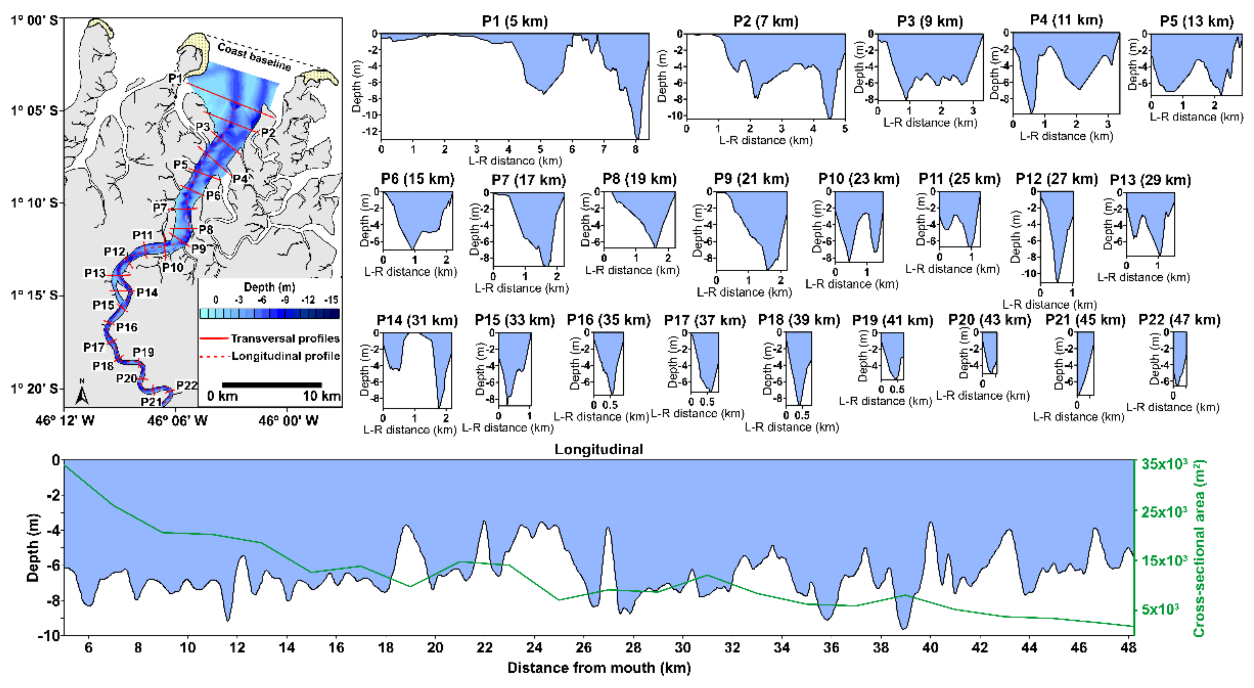
4.1. Estuarine Morphology
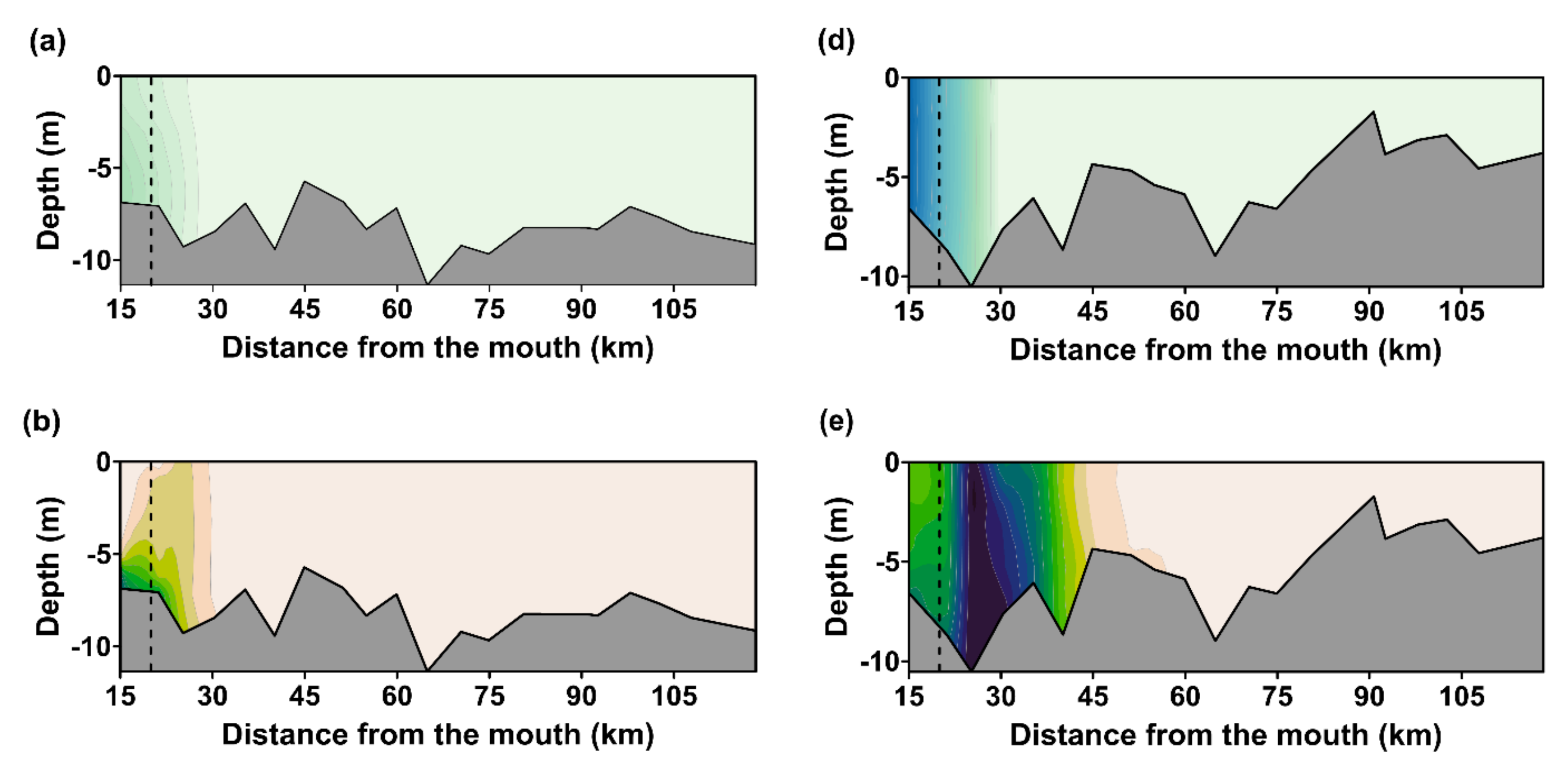
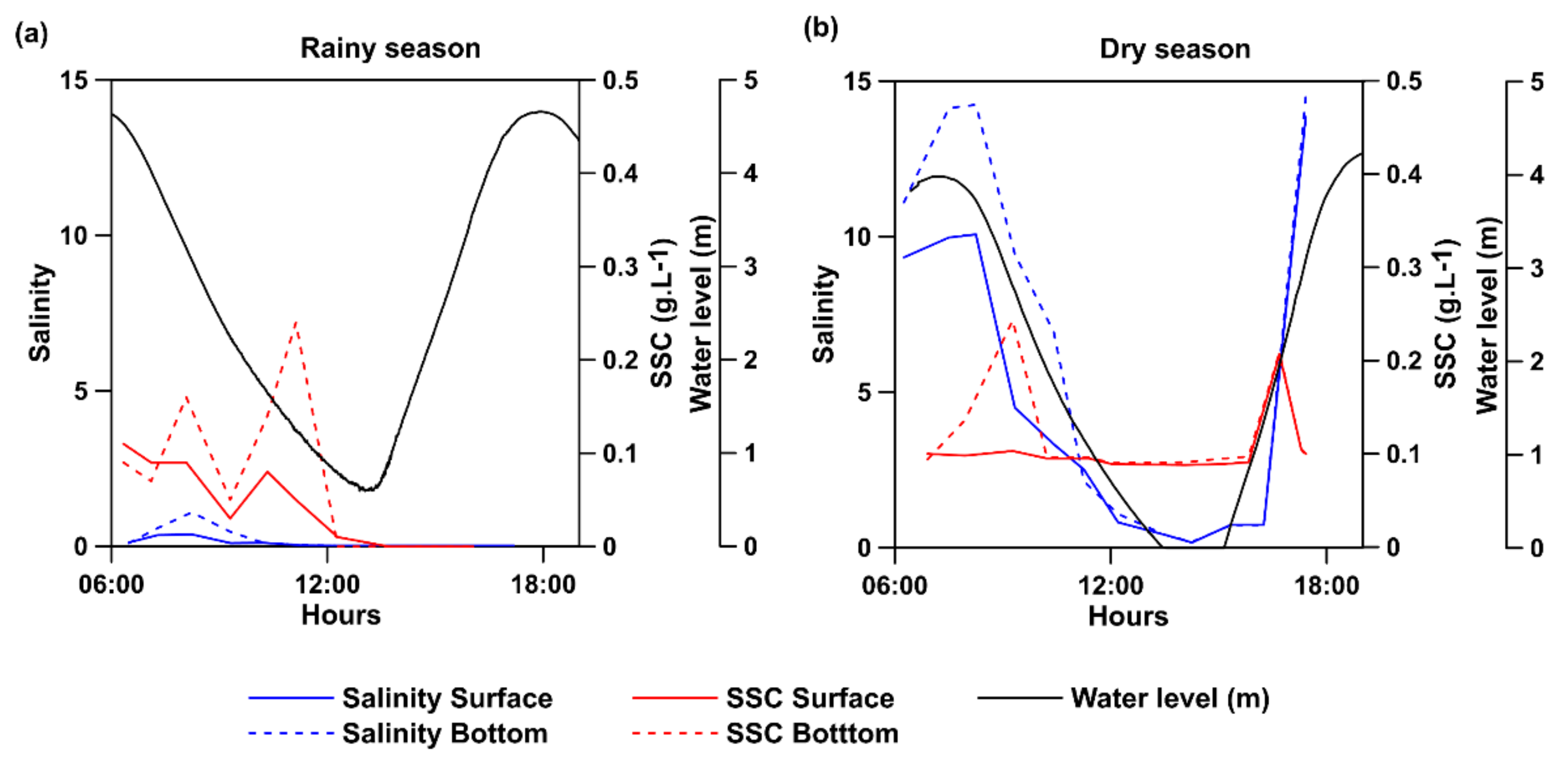
4.2. Suspended Sediment Concentration and Salinity
4.3. Tidal Patterns in Estuary Fluxes
4.4. Estuary Fluxes
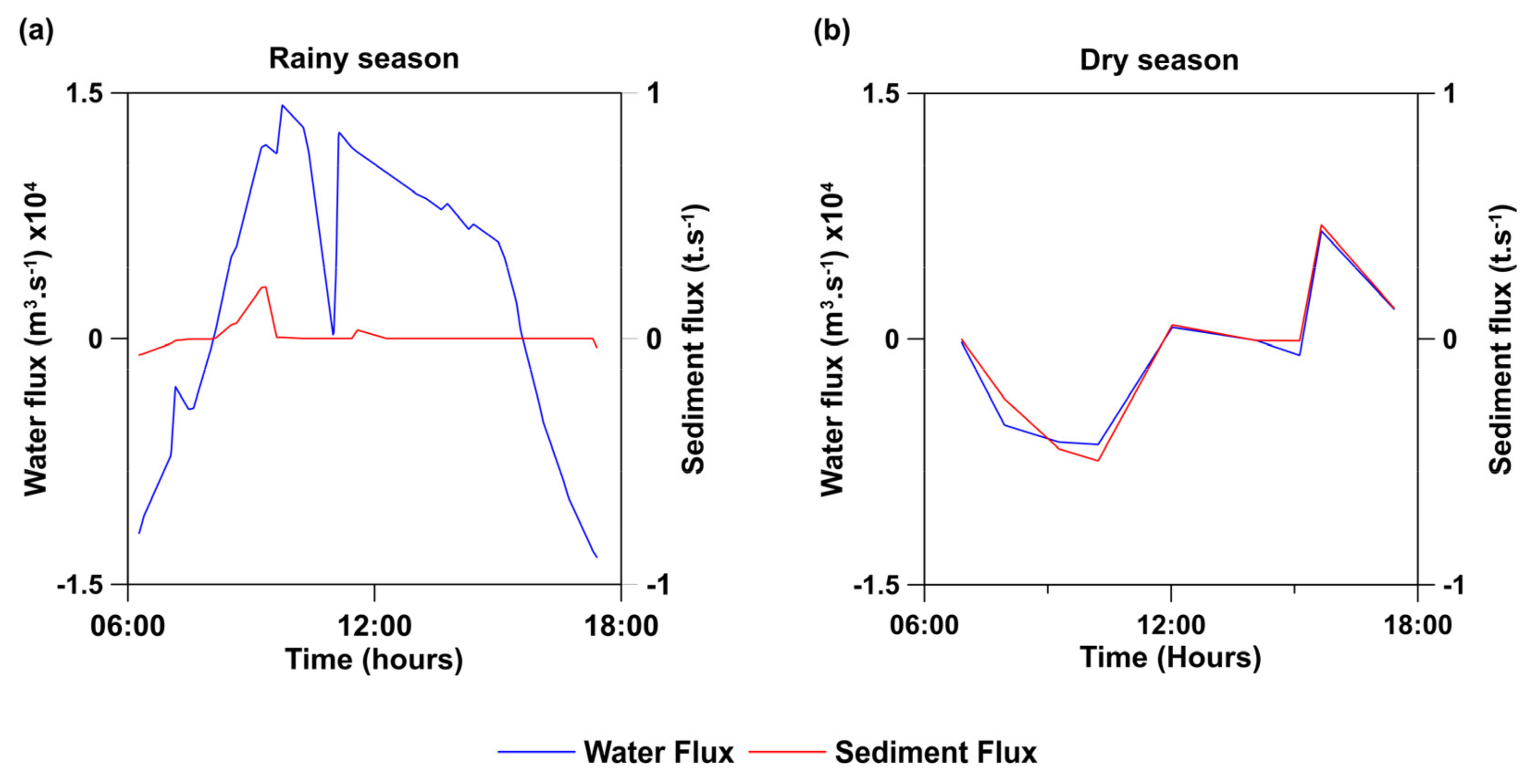
4.4.1. Net Water and Sediment Fluxes
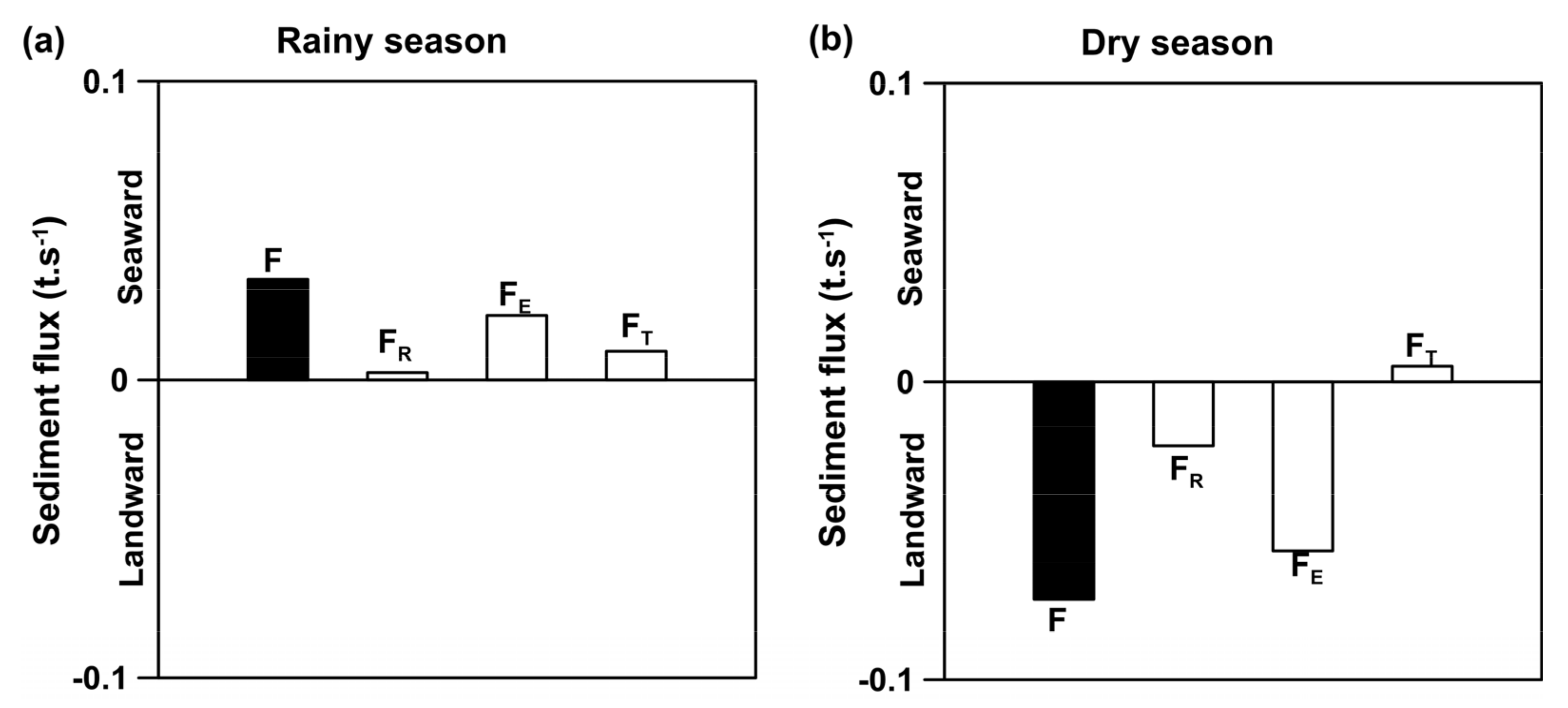
4.4.2. Sediment Flux Decomposition
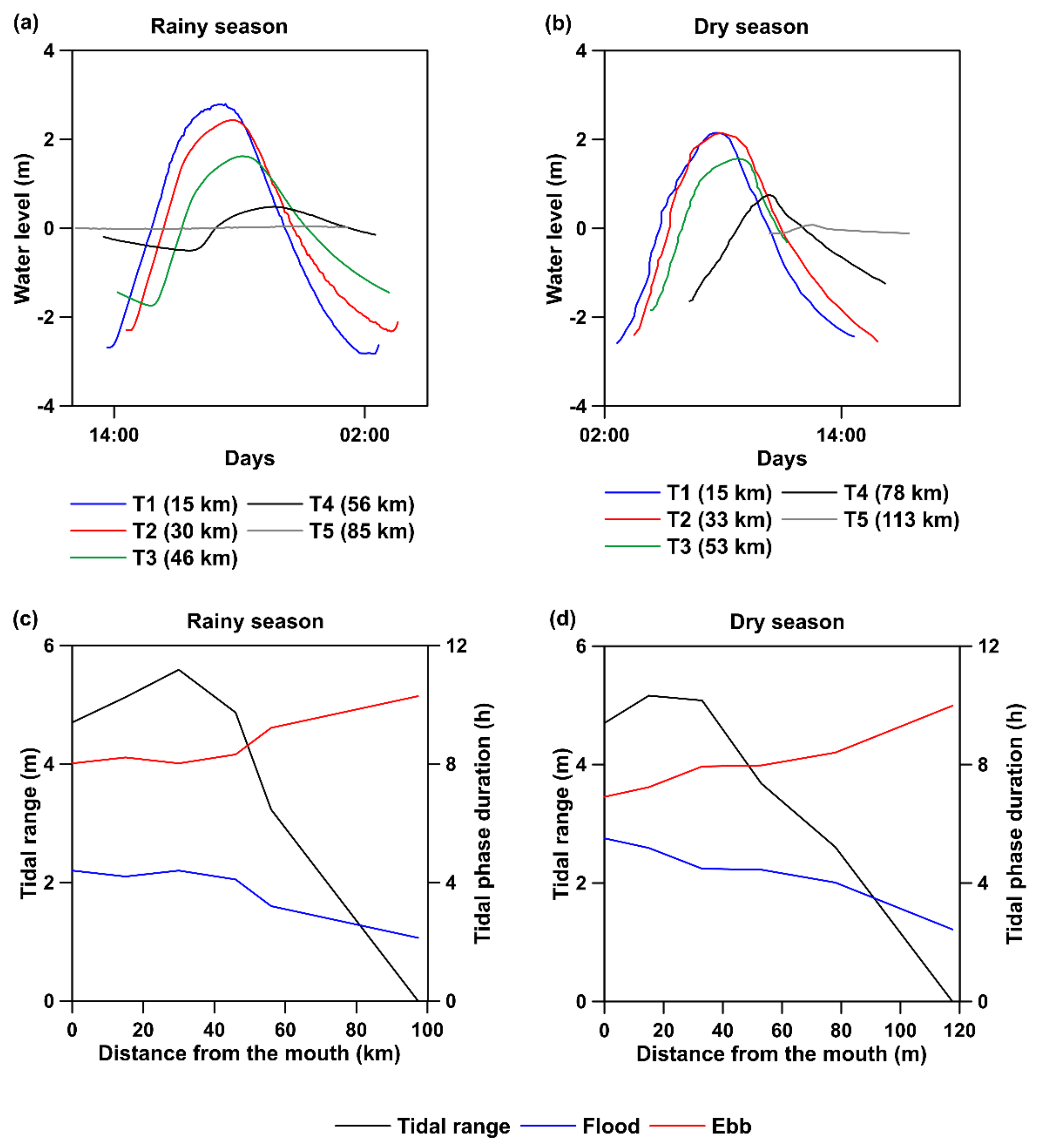
4.5. Tidal Propagation
5. Discussion
5.1. ETM Formation and Implications for Sediment Dynamics
5.2. Estuarine Circulation
5.3. Comparison to Other Amazonian Estuaries
6. Conclusions
Author Contributions
Funding
Data Availability Statement
Acknowledgments
Conflicts of Interest
References
- Syvitski, J.P.M.; Kettner, A. Sediment Flux and the Anthropocene. Philos. Trans. R. Soc. A Math. Phys. Eng. Sci. 2011, 369, 957–975. [Google Scholar] [CrossRef]
- Nowacki, D.J.; Ogston, A.S.; Nittrouer, C.A.; Fricke, A.T.; Van, P.D.T. Sediment Dynamics in the Lower Mekong River: Transition from Tidal River to Estuary. J. Geophys. Res. Ocean 2015, 120, 6363–6383. [Google Scholar] [CrossRef]
- Milliman, J.D.; Farnsworth, K.L. River Discharge to the Coastal Ocean: A Global Synthesis; Cambridge University Press: Cambridge, UK, 2011. [Google Scholar]
- Meade, R.H.; Nordin, C.F.; Curtis, W.F.; Costa Rodrigues, F.M.; do Vale, C.M.; Edmond, J.M. Sediment Loads in the Amazon River. Nature 1979, 278, 161–163. [Google Scholar] [CrossRef]
- Souza Filho, P.W.M. Costa de Manguezais de Macromaré Da Amazônia: Cenários Morfológicos, Mapeamento e Quantificação de Áreas Usando Dados de Sensores Remotos. Rev. Bras. Geofís. 2005, 23, 427–435. [Google Scholar] [CrossRef]
- Asp, N.E.; Gomes, V.J.C.; Schettini, C.A.F.; Souza-Filho, P.W.M.; Siegle, E.; Ogston, A.S.; Nittrouer, C.A.; Silva, J.N.S.; Nascimento, W.R.; Souza, S.R.; et al. Sediment Dynamics of a Tropical Tide-Dominated Estuary: Turbidity Maximum, Mangroves and the Role of the Amazon River Sediment Load. Estuar. Coast. Shelf Sci. 2018, 214, 10–24. [Google Scholar] [CrossRef]
- Souza Filho, P.W.M.; Lessa, G.C.; Cohen, M.C.L.; Costa, F.R.; Lara, R.J. The Subsiding Macrotidal Barrier Estuarine System of the Eastern Amazon Coast, Northern Brazil. In Geology and Geomorphology of Holocene Coastal Barriers of Brazil; Lecture Notes in Earth Sciences; Springer: Berlin/Heidelberg, Germany, 2009; Volume 107, pp. 347–375. ISBN 9783540250081. [Google Scholar]
- Cohen, M.C.L.; Souza Filho, P.W.M.; Lara, R.J.; Behling, H.; Angulo, R.J. A Model of Holocene Mangrove Development and Relative Sea-Level Changes on the Bragança Peninsula (Northern Brazil). Wetl. Ecol. Manag. 2005, 13, 433–443. [Google Scholar] [CrossRef]
- Sioli, H. The Amazon and Its Main Affluents: Hydrography, Morphology of the River Courses, and River Types. In The Amazon: Limnology and Landscape Ecology of a Mighty Tropical River and Its Basin; Sioli, H., Ed.; Springer: Dordrecht, The Netherlands, 1984; pp. 127–165. [Google Scholar]
- Copeland, B. Effects of Decreased River Flow on Estuary Ecology. Water Pollut. Control Fed. 1966, 38, 1831–1839. [Google Scholar]
- Ridderinkhof, H. Sediment Transport in Intertidal Areas. In Intertidal Deposits: River Mouths, Tidal Flats, and Coastal Lagoons; Eisma, D., Ed.; CRC Press: Boca Raton, FL, USA, 1998; pp. 363–382. ISBN 0-8493-8049-9. [Google Scholar]
- Zhang, E.; Savenije, H.H.G.; Wu, H.; Kong, Y.; Zhu, J. Analytical Solution for Salt Intrusion in the Yangtze Estuary, China. Estuar. Coast. Shelf Sci. 2011, 91, 492–501. [Google Scholar] [CrossRef]
- Zhang, E.F.; Savenije, H.H.G.; Chen, S.L.; Mao, X.H. An Analytical Solution for Tidal Propagation in the Yangtze Estuary, China. Hydrol. Earth Syst. Sci. 2012, 16, 3327–3339. [Google Scholar] [CrossRef]
- Cai, H.; Savenije, H.H.G.; Toffolon, M. Linking the River to the Estuary: Influence of River Discharge on Tidal Damping. Hydrol. Earth Syst. Sci. 2014, 18, 287–304. [Google Scholar] [CrossRef]
- Geyer, W.R.; MacCready, P. The Estuarine Circulation. Annu. Rev. Fluid. Mech. 2014, 46, 175–197. [Google Scholar] [CrossRef]
- Martins, E.D.S.F.; Souza Filho, P.W.M.; Costa, F.R.; Alves, P.J.O. Extração Automatizada e Caracterização Da Rede de Drenagem e Das Bacias Hidrográficas Do Nordeste Do Pará Ao Noroeste Do Maranhão a Partir de Imagens SRTM. In Proceedings of the 13 Simpósio Brasileiro de Sensoriamento Remoto, Florianópolis, Brazil, 21–26 April 2007; pp. 6827–6834. [Google Scholar]
- Asp, N.E.; Gomes, J.D.; Gomes, V.J.C.; Omachi, C.Y.; Silva, A.M.M.; Siegle, E.; Serrao, P.F.; Thompson, C.C.; Nogueira, L.C.; Francini-Filho, R.B.; et al. Water Column and Bottom Gradients on the Continental Shelf Eastward of the Amazon River Mouth and Implications for Mesophotic Reef Occurrence. J. Mar. Syst. 2022, 225, 103642. [Google Scholar] [CrossRef]
- Gomes, V.J.C.; Asp, N.E.; Siegle, E.; Gomes, J.D.; Silva, A.M.M.; Ogston, A.S.; Nittrouer, C.A. Suspended-Sediment Distribution Patterns in Tide-Dominated Estuaries on the Eastern Amazon Coast: Geomorphic Controls of Turbidity-Maxima Formation. Water 2021, 13, 1568. [Google Scholar] [CrossRef]
- Araújo, T.C.M.; Seoane, J.C.S.; Coutinho, P.N. Geomorfologia Da Plataforma Continental de Pernambuco. In Oceanografia: Um Cenário Tropical; Leça, E.E., Neumann-Leitão, S., Costa, M.F., Eds.; Bagaço: Recife, Brazil, 2004; pp. 39–57. [Google Scholar]
- Coles, V.J.; Brooks, M.T.; Hopkins, J.; Stukel, M.R.; Yager, P.L.; Hood, R.R. The Pathways and Properties of the Amazon River Plume in the Tropical North Atlantic Ocean. J. Geophys. Res. Ocean 2013, 118, 6894–6913. [Google Scholar] [CrossRef]
- Goes, J.I.; do Rosario Gomes, H.; Chekalyuk, A.M.; Carpenter, E.J.; Montoya, J.P.; Coles, V.J.; Yager, P.L.; Berelson, W.M.; Capone, D.G.; Foster, R.A.; et al. Influence of the Amazon River Discharge on the Biogeography of Phytoplankton Communities in the Western Tropical North Atlantic. Prog. Oceanogr. 2014, 120, 29–40. [Google Scholar] [CrossRef]
- Geyer, W.R.; Beardsley, R.C.; Lentz, S.J.; Candela, J.; Limeburner, R.; Johns, W.E.; Castro, B.M.; Soares, I.D. Physical Oceanography of the Amazon Shelf. Cont. Shelf Res. 1996, 16, 575–616. [Google Scholar] [CrossRef]
- Nittrouer, C.A.; Kuehl, S.A.; Sternberg, R.W.; Figueiredo, A.G.; Faria, L.E.C. An Introduction to the Geological Significance of Sediment Transport and Accumulation on the Amazon Continental Shelf. Mar. Geol. 1995, 125, 177–192. [Google Scholar] [CrossRef]
- Asp, N.E.; Gomes, V.J.C.; Ogston, A.; Borges, J.C.C.; Nittrouer, C.A. Sediment Source, Turbidity Maximum, and Implications for Mud Exchange between Channel and Mangroves in an Amazonian Estuary. Ocean Dyn. 2016, 66, 285–297. [Google Scholar] [CrossRef]
- Asp, N.E.; Amorim de Freitas, P.T.; Gomes, V.J.C.; Gomes, J.D. Hydrodynamic Overview and Seasonal Variation of Estuaries at the Eastern Sector of the Amazonian Coast. J. Coast. Res. 2013, 165, 1092–1097. [Google Scholar] [CrossRef]
- Cohen, M.C.L.; Lara, R.J.; Ramos, J.D.F.; Dittmar, T. Factors Influencing the Variability of Mg, Ca and K in Waters of a Mangrove Creek in Braganca, North Brazil. Mangroves Salt Marshes 1999, 3, 9–15. [Google Scholar] [CrossRef]
- Pereira, C.T.C.; Giarrizzo, T.; Jesus, A.J.S.; Martinelli, J.M. Caracterização Do Efluente de Cultivo de Litopenaeus Vannamei No Estuário Do Rio Curuçá (PA). In Sistemas de Cultivos Aqüícolas na Zona Costeira do Brasil: Recursos, Tecnologias, Aspectos Ambientais e Sócio-Econômicos; Barroso, G.F., Poersch, L.H.S., Cavalli, R.O., Eds.; Editora do Museu Nacional: Rio de Janeiro, Brazil, 2007; pp. 291–301. [Google Scholar]
- Lima, I.F.; Prata, T.C.; Maria, A.; Lima, M. de Análise Da Paisagem Aplicada a Bacia Do Rio Gurupi Pa/Ma. In Proceedings of the XXII Simpósio Brasileiro de Recursos Hídricos, Florianópolis, Brazil, 16 November–1 December 2017; pp. 1–8. [Google Scholar]
- Gomes, J.D. Caracterização Hidrodinâmica Do Estuário Do Rio Gurupi, Na Zona Costeira Amazônica; Universidade Federal do Pará: Belém, Brazil, 2015. [Google Scholar]
- Figueroa, S.N.; Nobre, C.A. Precipitations Distribution over Central and Western Tropical South América. Climanál.-Bol. Monit. Anál. Clim. 1990, 5, 36–45. [Google Scholar]
- Marengo, J.A. Interannual Variability of Deep Convection over the Tropical South American Sector as Deduced from ISCCP C2 Data. Int. J. Climatol. 1995, 15, 995–1010. [Google Scholar] [CrossRef]
- de Moraes, B.C.; da Costa, J.M.N.; da Costa, A.C.L.; Costa, M.H. Variação Espacial e Temporal Da Precipitação No Estado Do Pará. Acta Amaz. 2005, 35, 207–214. [Google Scholar] [CrossRef]
- Gomes, V.J.C.; Freitas, P.T.A.; Asp, N.E. Dynamics and Seasonality of the Middle Sector of a Macrotidal Estuary. J. Coast Res. 2013, 165, 1140–1145. [Google Scholar] [CrossRef]
- ANA—Agência Nacional de Águas. Hidroweb: Serviço de Informações Hidrológicas. Available online: http://www3.ana.gov.br (accessed on 11 December 2020).
- Strickland, J.D.H.; Parsons, T.R. A Practical Handbook of Seawater Analysis, 2nd ed.; Fisheries Research Board of Canada Bulletin: Ottawa, ON, Canada, 1972; Volume 167. [Google Scholar]
- Glover, H.E.; Ogston, A.S.; Fricke, A.T.; Nittrouer, C.A.; Aung, C.; Naing, T.; Kyu Kyu, K.; Htike, H. Connecting Sediment Retention to Distributary-Channel Hydrodynamics and Sediment Dynamics in a Tide-Dominated Delta: The Ayeyarwady Delta, Myanmar. J. Geophys. Res. Earth Surf. 2021, 126, e2020JF005882. [Google Scholar] [CrossRef]
- Giddings, S.N.; Monismith, S.G.; Fong, D.A.; Stacey, M.T. Using Depth-Normalized Coordinates to Examine Mass Transport Residual Circulation in Estuaries with Large Tidal Amplitude Relative to the Mean Depth. J. Phys. Ocean 2014, 44, 128–148. [Google Scholar] [CrossRef]
- McLachlan, R.L.; Ogston, A.S.; Allison, M.A. Implications of Tidally-Varying Bed Stress and Intermittent Estuarine Stratification on Fine-Sediment Dynamics through the Mekong’s Tidal River to Estuarine Reach. Cont. Shelf Res. 2017, 147, 27–37. [Google Scholar] [CrossRef]
- Lerczak, J.A.; Geyer, W.R.; Chant, R.J. Mechanisms Driving the Time-Dependent Salt Flux in a Partially Stratified Estuary. J. Phys. Ocean 2006, 36, 2296–2311. [Google Scholar] [CrossRef]
- Sternberg, R.W. Friction Factors in Tidal Channels with Differing Bed Roughness. Mar. Geol. 1968, 6, 243–260. [Google Scholar] [CrossRef]
- Ginestet, C. Ggplot2: Elegant Graphics for Data Analysis. J. Stat. Softw. 2009, 35, 245. [Google Scholar] [CrossRef]
- Oksanen, J. Vegan: An Introduction to Ordination. Management 2008, 1, 1–10. [Google Scholar]
- R Core Team. A Language and Environment for Statistical Computing; R Foundation for Statistical Computing: Vienna, Austria, 2020. [Google Scholar]
- Royston, P. Approximating the Shapiro-Wilk W-Test for Non-Normality. Stat. Comput. 1992, 2, 117–119. [Google Scholar] [CrossRef]
- Sheskin, D.J. The Mann–Whitney U Test. In Handb. Parametr. Nonparametric Stat. Proced, 5th ed.; Sheskin, D.J., Ed.; Chapman and Hall/CRC: New York, NY, USA, 2011; pp. 531–594. [Google Scholar] [CrossRef]
- Wilcoxon, F. Individual Comparisons by Ranking Methods. In Breakthroughs in Statistics; Springer: New York, NY, USA, 1992; pp. 196–202. [Google Scholar]
- Wu, J.; Liu, J.T.; Wang, X. Sediment Trapping of Turbidity Maxima in the Changjiang Estuary. Mar. Geol. 2012, 303–306, 14–25. [Google Scholar] [CrossRef]
- Dyer, K.R. Estuaries: A Physical Introduction, 2nd ed.; Wiley-Interscience Publication; John Wiley and Sons: New York, NY, USA, 1997; ISBN 0-471-9741-4. [Google Scholar]
- Allen, G.P.; Salomon, J.C.; Bassoullet, P.; du Penhoat, Y.; de Grandpre, C. Effects of Tides on Mixing and Suspended Sediment Transport in Macrotidal Estuaries. Sediment. Geol. 1980, 26, 69–90. [Google Scholar] [CrossRef]
- Jay, D.A.; Dungan Smith, J.; Jay, D.; SMrrH, J. Circulation, Density Distribution and Neap-Spring Transitions in the Columbia River Estuary. Prog. Oceanogr. 1990, 25, 81–112. [Google Scholar] [CrossRef]
- Uncles, R.J.; Stephens, J.A.; Law, D.J. Turbidity Maximum in the Macrotidal, Highly Turbid Humber Estuary, UK: Flocs, Fluid Mud, Stationary Suspensions and Tidal Bores. Estuar. Coast. Shelf Sci. 2006, 67, 30–52. [Google Scholar] [CrossRef]
- Valerio, A.M.; Kampel, M.; Ward, N.D.; Sawakuchi, H.O.; Cunha, A.C.; Richey, J.E. CO2 Partial Pressure and Fluxes in the Amazon River Plume Using in Situ and Remote Sensing Data. Cont. Shelf Res. 2021, 215, 104348. [Google Scholar] [CrossRef]
- Silva, A.M.M.; Asp, N.E.; Gomes, V.J.C.; Ogston, A.S. Impacts of Inherited Morphology and Offshore Suspended-Sediment Load in an Amazon Estuary. Estuar. Coasts 2023. (under review). [Google Scholar]
- Geyer, W.R. Estuarine Salinity Structure and Circulation. In Contemporary Issues in Estuarine Physics; Valle-Levinson, A., Ed.; Cambridge University Press: Cambridge, UK, 2010; pp. 22–26. [Google Scholar]
- Hansen, D.V.; Rattray, M. New Dimensions in Estuary Classification. Limnol. Oceanogr. 1966, 11, 319–326. [Google Scholar] [CrossRef]
- Valle-Levinson, A. Definition and Classification of Estuaries. In Contemporary Issues in Estuarine Physics; Valle-Levinson, A., Ed.; Cambridge University Press: Cambridge, UK, 2010; pp. 1–11. [Google Scholar]
- Farmer, D.M.; Freeland, H.J. The Physical Oceanography of Fjords. Prog. Oceanogr. 1983, 12, 147–220. [Google Scholar] [CrossRef]
- Lessa, G.C.; Santos, F.M.; Souza Filho, P.W.; Corrêa-Gomes, L.C. Brazilian Estuaries: A Geomorphologic and Oceanographic Perspective. In Brazilian Estuaries: A Benthic Perspective; Lana, P.D.C., Bernardino, A.F., Eds.; Springer International Publishing: Cham, Switzerland, 2018; pp. 1–37. ISBN 978-3-319-77779-5. [Google Scholar]
- Chappell, J.; Woodroffe, C.D. Macrotidal Estuaries. In Coastal Evolution: Late Quaternary Shoreline Morphodynamics; Carter, R.W.G., Woodroffe, C.D., Eds.; Cambridge University Press: Cambridge, UK, 1994; pp. 187–218. [Google Scholar]
- Dronkers, J. Tidal Asymmetry and Estuarine Morphology. Neth. J. Sea Res. 1986, 20, 117–131. [Google Scholar] [CrossRef]
- Kang, J.W.; Jun, K.S. Flood and Ebb Dominance in Estuaries in Korea. Estuar. Coast. Shelf Sci. 2003, 56, 187–196. [Google Scholar] [CrossRef]
- Aubrey, D.G.; Speer, P.E. A Study of Non-Linear Tidal Propagation in Shallow Inlet/Estuarine Systems Part I: Observations. Estuar. Coast Shelf. Sci. 1985, 21, 185–205. [Google Scholar] [CrossRef]
- Brown, J.M.; Davies, A.G. Flood/Ebb Tidal Asymmetry in a Shallow Sandy Estuary and the Impact on Net Sand Transport. Geomorphology 2010, 114, 431–439. [Google Scholar] [CrossRef]
- Friedrichs, C.T.; Aubrey, D.G. Nonlinear Tidal Distortion in Shallow Well-Mixed Estuaries. Estuar. Coast Shelf. Sci. 1988, 27, 521–545. [Google Scholar] [CrossRef]


Disclaimer/Publisher’s Note: The statements, opinions and data contained in all publications are solely those of the individual author(s) and contributor(s) and not of MDPI and/or the editor(s). MDPI and/or the editor(s) disclaim responsibility for any injury to people or property resulting from any ideas, methods, instructions or products referred to in the content. |
© 2023 by the authors. Licensee MDPI, Basel, Switzerland. This article is an open access article distributed under the terms and conditions of the Creative Commons Attribution (CC BY) license (https://creativecommons.org/licenses/by/4.0/).
Share and Cite
Silva, A.M.M.; Glover, H.E.; Josten, M.E.; Gomes, V.J.C.; Ogston, A.S.; Asp, N.E. Implications of a Large River Discharge on the Dynamics of a Tide-Dominated Amazonian Estuary. Water 2023, 15, 849. https://doi.org/10.3390/w15050849
Silva AMM, Glover HE, Josten ME, Gomes VJC, Ogston AS, Asp NE. Implications of a Large River Discharge on the Dynamics of a Tide-Dominated Amazonian Estuary. Water. 2023; 15(5):849. https://doi.org/10.3390/w15050849
Chicago/Turabian StyleSilva, Ariane M. M., Hannah E. Glover, Mariah E. Josten, Vando J. C. Gomes, Andrea S. Ogston, and Nils E. Asp. 2023. "Implications of a Large River Discharge on the Dynamics of a Tide-Dominated Amazonian Estuary" Water 15, no. 5: 849. https://doi.org/10.3390/w15050849
APA StyleSilva, A. M. M., Glover, H. E., Josten, M. E., Gomes, V. J. C., Ogston, A. S., & Asp, N. E. (2023). Implications of a Large River Discharge on the Dynamics of a Tide-Dominated Amazonian Estuary. Water, 15(5), 849. https://doi.org/10.3390/w15050849