Article

Simulation of Hydrologic Change of Linggo Co during 1979–2012 Using Hydrologic and Isotopic Mass Balance Model

1
College of Earth Science, Hebei GEO University, Shijiazhuang 050031, China
2
Key Laboratory of Cenozoic Geology and Environment, Institute of Geology and Geophysics, Chinese Academy of Sciences, Beijing 100029, China
*
Author to whom correspondence should be addressed.
Water 2023, 15(5), 1004; https://doi.org/10.3390/w15051004
Submission received: 2 February 2023 / Revised: 2 March 2023 / Accepted: 4 March 2023 / Published: 6 March 2023
(This article belongs to the Section Hydrogeology)

Abstract

:
The Tibetan Plateau (TP) and surrounding areas contain the largest number of glaciers outside the polar regions. The region affects downstream water supply and food security, thereby directly influencing one-third of the world’s population. The lakes in the central TP expanded rapidly in recent decades, which has attracted growing attention. Glacier meltwater was considered as a major component in the water balance of TP lakes, although few studies quantified its contribution. Stable isotope analysis is a powerful tool to trace hydrologic circulation, while its interpretation in paleoclimate records has been controversial. To bridge the gap between hydrologic and paleoclimatic studies, we performed a hydrologic and isotopic mass balance model to simulate the lake level change of Linggo Co in the central TP. The model was forced by the meteorological data, calibrated through observed lake level changes, and validated by oxygen isotope compositions (δ18O) of lake water. Our results indicated that glacier meltwater contributed 73.94% of the inflow water to Linggo Co before 1993 but decreased thereafter. Increasing glacier meltwater together with positive water balance (precipitation/evaporation) in the catchment contributed to the rapid expansion of Linggo Co after the mid-1990s. Lake water δ18O in Linggo Co was more sensitive to changes in the precipitation amount and precipitation δ18O than temperature. Our findings could shed light on the usage of δ18O proxy in future paleoclimate research on the TP.

1. Introduction

The Tibetan Plateau (TP) and surrounding areas contain the largest number of glaciers outside the polar regions [1]. The water resources on the TP affect downstream water supply and food security, thereby directly influencing one-third of the world’s population [2,3,4]. In recent decades, the TP has undergone significant warming, along with remarkable changes in the hydrosphere [2,5]. Major lakes in the central TP have expanded since the 1990s, whereas many lakes in the southern TP have shrunk [5,6,7,8,9]. The reasons for lake variations in the TP have been widely discussed [1,2,7]. Among various factors (e.g., glacier melt, precipitation, and potential evaporation), glacier melt was the most frequently invoked contributor [1,6,9,10]. However, only a few studies quantified its contribution to the lake water budget [7,11,12], which is critical for understanding the interactions between cryosphere and hydrosphere and the response of lake dynamics to climate change.
Stable isotope analysis has long been considered a powerful tool to reconstruct the paleoclimate [13,14,15,16,17] and hydrological change [18,19,20,21,22,23]. For a lake system, oxygen isotope compositions (δ18O) of lacustrine carbonates were controlled by isotopic compositions of lake water, which in turn responded to hydrological changes driven by climate change [18,24]. Increasing temperature would enhance evaporation on the lake surface and catchment, leading to 18O enrichment of lake water [18]. Increasing precipitation amount would alter the isotopic composition of inflowing river, thus the δ18O of lake water [18]. Moreover, δ18O of precipitation was associated with temperature and precipitation amount due to the so-called “temperature effect” and “amount effect” [18]. The interpretation of δ18O record on the TP is even more complex since many lakes on the TP are located in a close basin with strong evaporation, and received multi-source water (glacier meltwater, summer monsoon, or mid-latitude westerlies induced moisture) with distinguished isotopic compositions [25,26]. Quantitatively assessing the influence of these factors, such as temperature, precipitation amount, and isotopic compositions of precipitation on the isotopic composition of lake water, can shed light on the interpretation of stable isotope proxies in paleoclimate reconstruction on the TP.
Linggo Co (Figure 1) is a close basin lake in the central TP [27]. It is fed primarily by meltwater from the Purogangri ice sheet [28]. Remote sensing-based investigations have suggested large lake level variations in recent decades [10]. δ18O records of ostracod shells have revealed a sharp 4‰ shift at the beginning of the Holocene [29]. For a better understanding of this isotopic variation, we performed a hydrologic and isotope mass balance model of Linggo Co. The model was forced by meteorological data from 1979 to 2012, calibrated by the lake area change, and validated by lake volume and lake water δ18O measurements. Sensitivity analyses were conducted on temperature, precipitation amount, and precipitation δ18O. The main objectives of this study are to (1) quantify the contribution of glacier meltwater to the expansion of Linggo Co and (2) access the effects of temperature, precipitation amount, and precipitation δ18O on lake water δ18O.

2. Materials and Methods

2.1. Geological Settings

Linggo Co (88°31′–88°39′ E, 33°48′–33°54′ N, 5059 m a.s.l.) is located within a 1830 km2 closed basin in the central TP (Figure 1). The Puruogangri ice sheet to the east of the watershed has an extent of ~422.6 km2, of which ~135 km2 lies in the catchment of Linggo Co [27]. Small seasonal rivers, which are supplied by the meltwater from Puruogangri ice sheet in the summer, flow over the Gobi zone in the piedmont and drain into Linggo Co [28]. The lake area is characterized by a sub-frigid semi-arid climate. Based on the observations from October 2011 to September 2013 [30], the mean annual temperature is about −4 °C, with a high monthly temperature of about 7 °C in July and a low of about −15 °C in January. The annual precipitation, which mainly falls from June to September, is ~333 mm. Actual evapotranspiration is close to the annual precipitation, while the mean annual potential evaporation is ~1000 mm [30,31].

2.2. Data Source and Structure of the Model

The meteorological data of the model mainly came from the China Meteorological Forcing Dataset (CMFD, http://westdc.westgis.ac.cn/ (accessed on 16 May 2015)), which was produced by merging a variety of data sources (including China Meteorological Administration (CMA) station data, TRMM satellite precipitation data (3B42), and the GLDAS precipitation data) with the spatial and temporal resolutions of 3 h and 0.1°*0.1°, respectively [32,33]. In order to assess the data quality, the CMFD data were compared to the High Asia Refined Reanalysis Dataset (HAR, http:// www.klima-ds.tu-berlin.de/har/ (accessed on 14 June 2015)) [34] and CMA station observed data (temperature, wind speed, relative humidity, and precipitation) from five stations around our study area (Shenza, Gaize, Naqu, Bange, and Amduo; Supplementary Figures S1–S4). Considering the overestimation of precipitation in the monsoon season (from May to October) of the CMFD data after 2000 (Supplementary Figure S1), CMFD data were combined with HAR data from May to October during 2000–2012 (Supplementary Figure S5).
Glacier albedo was extracted from HAR data [34]. Glacier meltwater δ18O was based on the average value of Puruogangri ice core (−12.5‰, [35]). Sunshine hours data came from CMA data [36]. The lake area was extracted using remote sensing and GIS techniques [10]. The bathymetry map was measured in the field in 2011 and digitized using ArcGIS software to extract the area at the surface and bottom. Monthly precipitation δ18O was extracted using the Online Isotopes in Precipitation Calculator (Version 2.2, [37]). One lake water sample was collected near the northern shore of the lake (red dot in Figure 1) on May 25th, 2015, by Dr. Yanbin Lei from Institute of Tibetan Plateau Research, Chinese Academy of Sciences (ITPCAS), and oxygen isotope was analyzed in the Key Laboratory of Tibetan Environment Changes and Land Surface Processes, ITPCAS (personal communication).

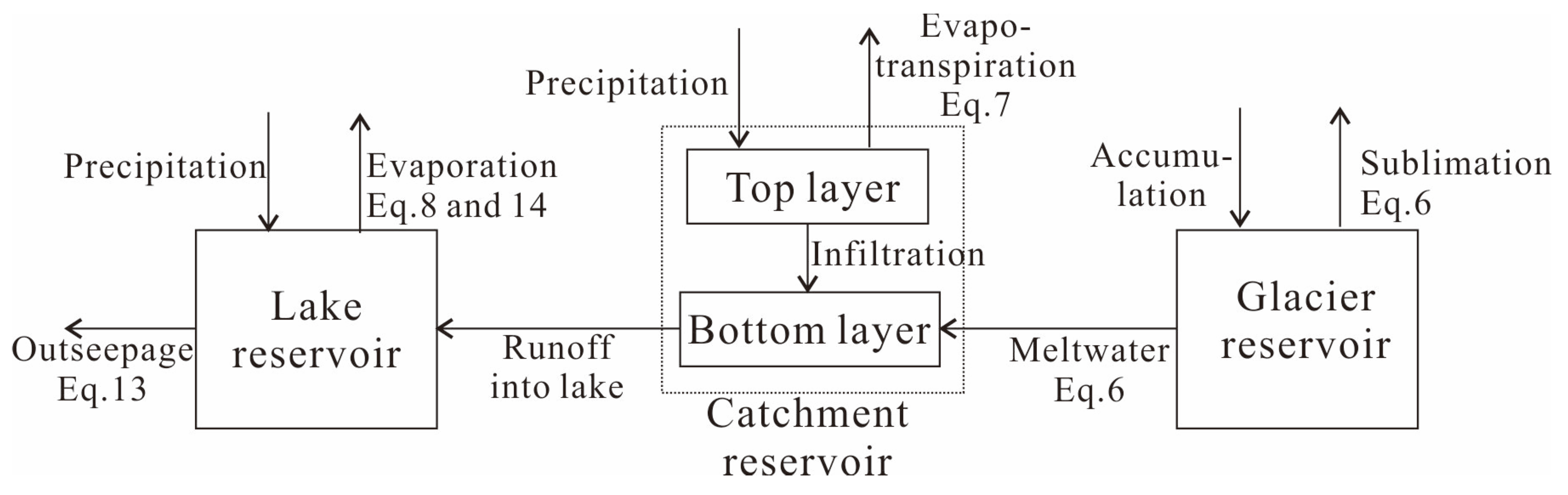
2.3. Model Structure

The hydrologic and isotope mass balance model of Linggo Co is simplified after Steinman [22,23]. The model is described using the following equations:
d V L d t =   I     O  
d ( V L δ L ) d t     =   I   ×   δ I     O   ×   δ O  
where VL is the reservoir volume, ∑I and ∑O are the total inflows and outflows from the reservoir, and δ is the isotopic composition of the inflows and outflows. The hydrologic model is defined by three separate equations, each corresponding to a different water reservoir: the glacier, catchment, and lake (Figure 2).

2.3.1. Glacier Reservoir

There are three processes that occur at the glacier surface: melting, accumulation, and sublimation. The glacier mass balance is based on energy balance methods [38]. The energy at the surface–air interface is expressed as:
QN + QH + QL + QG + QR + QM = 0
where QN is the net radiation, QH is the sensible heat flux, QL is the latent heat flux (QH and QL are referred to as turbulent heat fluxes), QG is the ground heat flux, QR is the sensible heat flux supplied by rain, and QM is the energy consumed by melt. The QN represents the majority of the energy based on the observation in the TP (Zhadang glacier: 82% [39]; Qiyi glacier: 90% [40]). Therefore, we use QN as the melt energy in this work.
Q N   = G   ×   ( 1 α ) + L   + L
where G is the global radiation, α is the surface albedo, L is the downward longwave radiation, and L is the upward longwave radiation which can be calculated as:
L   =   ε σ T 4
where ε is the emissivity; σ = 5.67 × 10⁸ Wm2 K−4 which is known as Stefan–Boltzmann constant [38]. For melting surface, the L = 316W*m−2. If the melt energy (QN) is less than zero, all the precipitation/snow is accumulated, while if the energy is greater than zero, the melt rate, M, is then computed from the available energy by:
M = Q M ρ W × L f
where ρW denotes the density of water; Lf = 334,000 J*kg1 stands for the latent heat of fusion. The sublimation is also calculated by the above equation. The difference is the energy for sublimation, which is 2,848,000 J*kg1.

2.3.2. Catchment Reservoir

The catchment is described as a two-layer soil model. Precipitation and evapotranspiration occur within the top soil. The deep soil receives glacier meltwater, which experiences a brief exposure time before evaporating and forming runoff. In the rainy season, if top soil receives more water than its maximum available water capacity, water in top soil may infiltrate into deep soil.
The actual evapotranspiration is calculated following Morton’s CRAE method [41]. This method is based on the hypothesis that, for large homogeneous areas where there is little advective heat and moisture, there is a complementary relationship (CR) between actual evaporation and potential evaporation:
ETact = 2ETwet − ETpot
where Tact is the actual areal or regional evapotranspiration from an area large enough that the heat and vapor fluxes are controlled by the evaporation power of lower atmosphere and unaffected by upwind transitions. ETwet is the potential evapotranspiration that would occur under steady-state meteorological conditions in which the soil/plant surface is saturated with abundant water. ETpot is the (point) potential evapotranspiration for an area so small that the heat and water vapor fluxes have no effect on the overpassing air. The CR relationship has been confirmed in the field observation at Shanghu area that is 60 km south of Linggo Co [42]. The details of the calculation process can be found in the study by McMahon et al. (2013) [43].

2.3.3. Lake Reservoir

Evaporation, precipitation, runoff, and outseepage occurred in the lake reservoir. The evaporation model applied in this paper is the simplified version of the modified Penman equation with elevation calibration proposed by Valiantzas (2006) [44]:
E = [ 0.051 × ( 1 ALB ) × R S × ( T a + 9.5 ) 1 2 2.4 × ( R S / R a ) 2 + 0.052 × ( T a + 20 ) × ( 1 RH / 100 ) × ( a u   0.38 + 0.54 × WS ) + 0.00012 ×   ELE ] × 30
where E is the evaporation in mm per month, ALB is the albedo of the lake (0.08), Ta is the average daily temperature in °C, RS is the solar radiation in MJ m2d−1, and Ra is the extraterrestrial radiation in MJ m2d1. RH is the average daily relative humidity expressed as a percentage, au is the Penman wind function constant, and WS is the average daily wind speed in ms1. ELE is the elevation of the lake. The evaporation is set to zero if Ta < 0. RS and Ra are calculated in the following equations:
RS = Ra × (0.5 + 0.25 × n/N)
N ≈ 4∅ sin(0.53i − 1.65) + 12
Ra ≈ 3N sin (0.131N − 0.95∅) for |∅| > 23.5π/180
Or Ra ≈ 118N0.2 sin (0.131N − 0.2∅) for |∅| < 23.5π/180
where n is the measured bright sunshine hours per day (h) and N is the maximum possible duration of daylight (h). ∅ is the latitude of the study site (radians), positive for the Northern Hemisphere and negative for the Southern Hemisphere. i is the rank of the month (the first month is January).
The outseepage function is based on the exponential relationship between lake radius and hydraulic conductivity values (K) described by Genereux et al. (2001) [45]:
K = A × ebR
where R is the radius of an ideal round lake. A and b are parameters that vary with different settings of lakes. We simplified the Linggo Co hypsographic profile to an upside-down frustum of a right circular cone (Supplementary Figure S6). Thus, the total hydraulic conductivity (Ktotal) can be expressed as:
K total = R 0 R 1 A × e bx × d x
where R0 and R1 are the radii at the bottom and surface of Linggo Co (Supplementary Figure S6). A and b are coupled parameters that needed to be adjusted in the model calibration.

2.3.4. Isotope Mass-Balance Equations

Oxygen isotope value, expressed in standard delta (δ) notation as the per mil (‰) relative to the standard Vienna Standard Mean Ocean Water (VSMOW), is calculated for each reservoir at each time step and is multiplied by the corresponding hydrologic flux to determine the isotope mass balance of each theoretical water mass.
The model of Craig et al. (1965) [46] is used to calculate the isotopic composition of water evaporating from the lake surface:
δ E = α * δ L h n δ A ε tot 1 h n + 0.001 ε k  
where α* is the reciprocal of the equilibrium isotopic fractionation factor, δ L is the isotopic composition of the lake water, h n is the ambient humidity normalized to lake water temperature, δ A is the isotopic composition of atmospheric moisture, and ε t o t is the total isotopic separation, which equals to ( ε e q + ε k ). ε e q is the equilibrium isotopic separation and ε k is the kinetic isotopic separation.
The saturation vapor pressure of the overlying air ( e s a ) and the saturation vapor pressure at the surface water temperature ( e s w ) in millibars are used to determine the normalized relative humidity ( h n ).
h n   = RH   ×   e s a / e s w
e s a or   e s w = 6.108 × e x p ( 17.27 ×   T T + 237.7 )
Atmospheric moisture ( δ A ) is assumed to be in isotopic equilibrium with precipitation [47]:
δ A   = δ A   ε eq
The equilibrium isotopic fractionation factor (α) and the reciprocal of the equilibrium isotopic fractionation factor (α*) for oxygen are calculated as [48]:
In α = 0.35041 × ( 10 6 T w 3 ) 1.6664 × ( 10 3 T w 2 ) + 6.7123 × ( 1 T w ) 7.685 × 10 3
where Tw is the temperature (degrees K) of the lake surface water. The lake surface temperature is assumed to be zero if the atmospheric Ta < 0; the lake surface temperature is 0.95× Ta before June, while it is equal to Ta after July. The per mil equilibrium separation ( ε e q ) of oxygen is calculated as:
ε eq = 1000 × ( 1 α * )
Kinetic fractionation ( ε k ) is controlled by molecular diffusion and moisture deficit (1 − h n ) over the lake surface:
ε k   =   C   × ( 1   h n )
where C is the experimentally derived isotopic separation value of 14.3‰ for oxygen that is applied.

2.3.5. Model Calibration and Sensitivity Analyses

All model simulations were conducted with Stella software using fourth-order Runge–Kutta numerical integration method. According to a previous study [10], lake area of Linggo Co changed from 94.75 km2 to 97.59 km2 from 1976 to 1992. Compared with the rapid lake expand rate thereafter, this period was relatively stable which was treated as hydrological steady status. Therefore, in the first step of calibration, the model was forced by monthly average data of 1979–1992 (Supplementary Table S1) and the adjusted parameters A and b in Equation (13) to make the simulated lake area close to the observed lake surface in September 1992 (97.59 km2). There are several combinations of A and b that corresponded to the single Ktotal (Table 1). In the second step of calibration, we forced the hydrological steady lake in the model using monthly data from 1979 to 2012. The combination of A and b was selected that made the simulated lake area in 1999 and 2006 as close to the observation as possible (Table 1). The validity of the model was testified by the difference in isotopic values of lake water between observation and simulation.
In order to determine the isotopic sensitivity of Linggo Co to temperature, precipitation amount, and isotopic composition of precipitation, two sets of sensitivity analyses at steady and transient states were conducted.
Simulation at steady state was conducted on monthly step over 500 model years using modern catchment parameters and the average climate data from 1979 to 1992. Between the 1601st and 2008th simulation month, the tested parameter was altered (increased or decreased) by a constant percent, according to its coefficient of variation over 1979–1992 (Supplementary Table S1).
Simulation at transient state was conducted on a monthly step over 234 model years. For the first 200 years, the model was forced by the average data from 1979 to 1992. From the 2401st to 2808th month (January of the 201st year), the model was forced by the monthly data from 1979 to 2012, except for the tested parameters which increase or decrease by the same amount as the previous sensitivity test. As for the isotopic composition of precipitation, it increased by 10% in the summer season (from June to August). The same amount of change and time allow the results of two sensitivity analyses to be compared.

3. Results

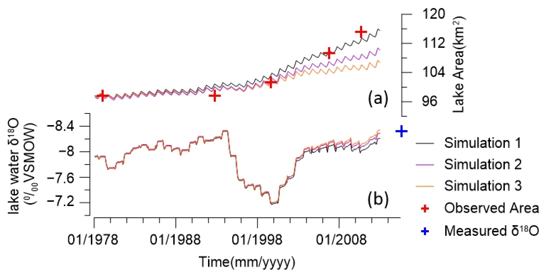
3.1. Model Calibration

The adjusted hydraulic conductivity after the first step of calibration is 0.055 m/month, which lies within the range of dense clay (<0.06 m/month [49]). After the second step of calibration, the values of A and b are chosen as (39.35, 0.0001), since the combination led to the closest simulated lake area in August 2010 with observation (Table 1). Moreover, the lake water isotope value at the end of 2012 is −8.22‰, which fits with the observed data (−8.32‰) in May 2015 after stretching (Figure 3), implying the validity of the model.
After two steps of calibration, we can reconstruct the continuous records of lake area changes during 1979–2012 and quantify the amount of each flux input/output to Linggo Co. The hydrological change of Linggo Co can be separated into three stages: insignificant expansion from 1979 to 1992, stable status from 1993 to 1996, and rapid expansion thereafter (Figure 3). Annual precipitation on Linggo Co ranged from 1.49 × 10⁷~4.95 × 10⁷ m3, runoff to Linggo Co had a wider variation from 9.34 × 10⁷~16.14 × 10⁷ m3 per year, evaporation over lake surface ranged from 5.48 × 10⁷~9.04 × 10⁷ m3 per year, and outseepage was relatively stable from 6.37 × 10⁷~7.55 × 10⁷ m3 per year. The net water budget (precipitation minus evaporation) in the catchment varied from 0.00~19.19 × 10⁷ m3 (Table 2).

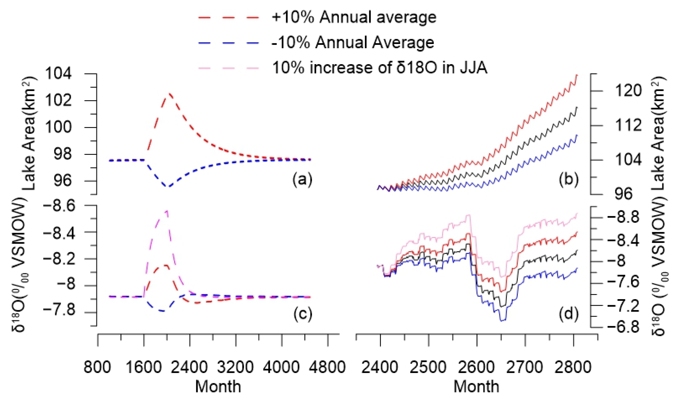
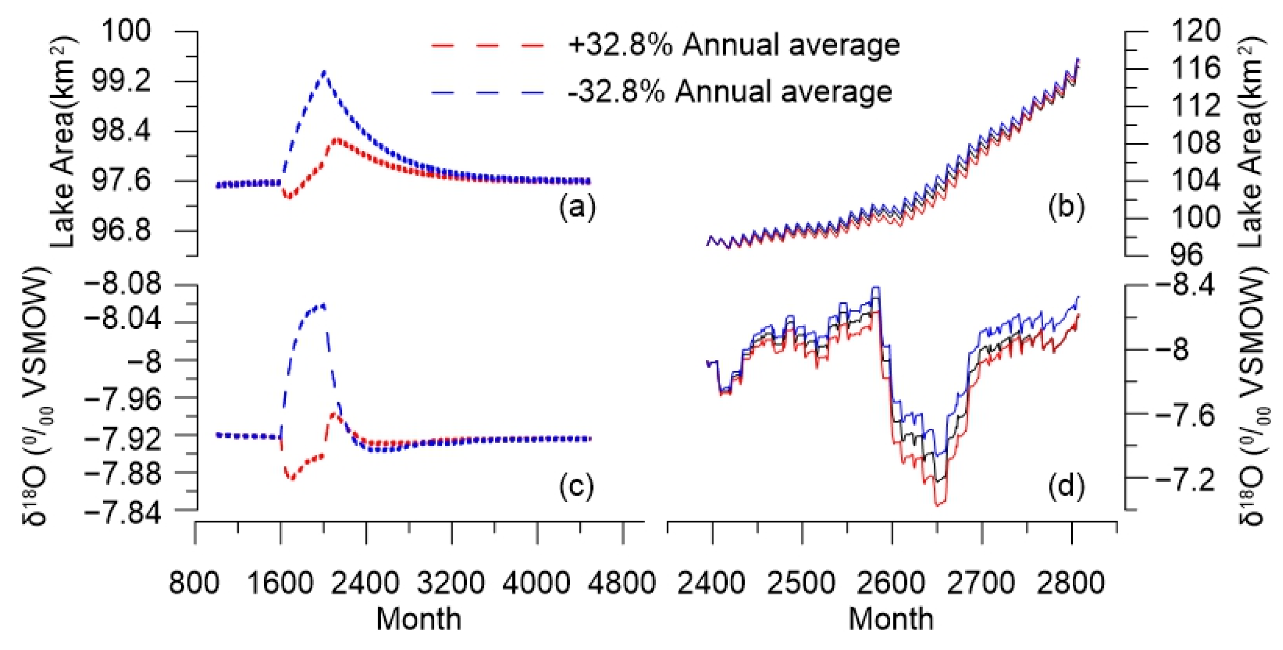
3.2. Sensitivity Analysis of Model

In response to the 10% increase in precipitation amount, the lake area at steady status expanded by ~5.3 km2, while by ~7.2 km2 at transient simulation (red curve in Figure 4a,b). Decreasing precipitation by 10% leads to lake area shrinking ~2.4 km2 at steady status and ~6.2 km2 at transient status (blue curve in Figure 4a,b). As for δ18O, increase by 10% in precipitation amount causes δ18O value to decrease by 0.25‰ at steady status and 0.33‰ at transient simulation (red curve in Figure 4c,d). A 10% decrease in precipitation causes δ18O value to increase 0.14‰ at steady status and 0.33‰ at transient simulation (blue curve in Figure 4c,d). δ18O value of precipitation in the summer (June–August) increasing by 10% (~0.15‰ in value) leads to a 0.65‰ shift at steady status and 0.67‰ at transient status (pink curve in Figure 4c,d).
A 32.8% increase in temperature led to the lake area shrinking in the first 5 months; after that, the lake expanded ~0.8 km2 at steady status. The δ18O experienced the same trend: increase in the first five months and then decrease. A 32.8% decrease in temperature, that decreased the actual evaporation as much as 0.30× 10⁷ m3 per year, gave rise to the lake expanding 2 km2 and δ18O decreasing 0.10‰. Little variation occurred in lake area and isotopic compositions under temperature changes in the transient simulation (Figure 5).

4. Discussion

4.1. The Role of Glacier Melt to Lake Expand in Recent Decades

Previous studies have suggested that many factors, such as glacier meltwater [10,50], precipitation [51], and potential evaporation [52,53,54], influence the water budget in the central TP. The difference between simulated results at steady and transient states can provide some guidance in calculating the water budget. In response to precipitation amount change, the variation of lake area at transient status was larger than that at steady status (Figure 4). It implies that the increase in precipitation alone cannot fully account for the lake expansion during the past decade. As the temperature changes, the lake area changes at both statuses are limited. It indicated that the increasing temperature can accelerate glacier melt, while its contribution to the water budget may be offset by enhanced evaporation at the same time.
As for the hydrologic change in Linggo Co, the trend that accelerated expansion in the mid-1990s is consistent with other closed lakes in the central TP [55]. The melt of Puruogangri ice sheet also increased from 0.75 × 10⁸ m3 in 1979 to 1.06 × 10⁸ m3 in 2012, which is also evidenced in others glacier in the TP [50]. From 1979 to 1993, glacier meltwater contributed 73.94% of the average inflow of water (runoff into lake plus precipitation on lake) to Linggo Co. From 1993 to 2012, the contribution of glacier meltwater to runoff decreased to 59.67% on average (Table 2, Figure 6). In other words, increasing glacier meltwater, together with positive water balance (precipitation/evaporation) in the catchment, contributed to the rapid expansion of Linggo Co after 1993.

4.2. The Isotopic Response of Linggo Co to Temperature and Precipitation Amount

The δ18O of lacustrine carbonates (e.g., ostracod shells), representing the δ18O composition of lake water, was widely used in paleoclimate studies in the TP [24]. The interpretation of this proxy varies, such as temperature variation [56], lake water balance that responds to the amount of monsoonal precipitation [57], and the interaction between Asian summer monsoon and mid-latitude westerlies [13,58]. The fundamental question is how the lake water δ18O responded to changes in temperature, precipitation amount, and precipitation δ18O.
Based on our sensitivity analysis results, isotopic composition of lake water in Linggo Co was least sensitive to temperature variation, relatively sensitive to precipitation amount, and sensitive to precipitation isotopic composition. These results could shed light on the interpretation of the ~4‰ shift in δ18O record of ostracod shells in Linggo Co in the early Holocene [29]. Increasing temperature could not explain this range of δ18O fluctuation. The precipitation amount would increase in response to enhanced Asian summer monsoon during the early Holocene. However, the increased precipitation amount may not be large enough to support the isotopic variation, considering that a 10% variation in precipitation amount led to 0.33‰ isotopic variation of lake water during 1979–2012. On the other hand, moisture induced by Asian summer monsoon and westerlies has large isotopic differences. For example, the δ18O difference of summer precipitation between Nagqu and Gaize is 6.4‰ (Nagqu: −17.0‰, Gaize: −10.6‰ [59]). Meanwhile, δ18O value of summer precipitation varies by ~0.15‰ and can lead to ~0.67‰ change in lake water δ18O value based on our sensitivity analyses. Thus, it is highly possible that the shift in δ18O records of Linggo Co was caused by a change in atmospheric circulation systems.

5. Conclusions

In this study, we first carried out the hydrologic and isotopic mass balance model in lakes on the TP. We simulated the hydrologic change of Linggo Co during 1979–2012 to quantify the contribution of glacier meltwater to the expansion of Linggo Co and assess the influences of temperature, precipitation amount, and precipitation isotopic composition on lake water isotopic composition. Our findings are as follows:
1. Hydrologic change of Linggo Co during 1979–2012 can be separated into two stages: before 1993, meltwater contributed 90% of the runoff, while after that, the contribution of glacier meltwater to runoff decreased to at least 49% (in 1999). Increasing glacier melting together with positive water balance (precipitation/evaporation) in the catchment contributed to the rapid expansion of Linggo Co.
2. Isotopic composition of lake water in Linggo Co was not sensitive to temperature variation, relatively sensitive to precipitation amount, and sensitive to precipitation isotopic composition. A large shift in δ18O record of Linggo Co during the early Holocene was caused by the interplay between Asian summer monsoon and mid-latitude westerlies.

Supplementary Materials

The following supporting information can be downloaded at: https://www.mdpi.com/article/10.3390/w15051004/s1. Figures S1–S4: Comparisons of CMFD data with observed data; Figure S5: Comparison of combined CMFD and HAR data with raw CMFD data; Figure S6: Simplified hypsographic profile of Linggo Co; and Table S1: Climatic parameters used in the model.

Author Contributions

Conceptualization, Y.H. and L.T.; methodology, Y.H.; software, Y.H.; validation, X.Z.; formal analysis, X.Z. and Y.H.; investigation, X.Z. and Y.H.; resources, H.D. and Y.C.; data curation, H.D. and Y.C.; writing—original draft preparation, X.Z.; writing—review and editing, Y.H. and L.T.; visualization, H.D and Y.C.; supervision, Y.H.; project administration, Y.H.; funding acquisition, Y.H. and L.T. All authors have read and agreed to the published version of the manuscript.

Funding

This research was funded by the National Natural Science Foundation of China (Grant No. 42106228) and Natural Science Foundation of Hebei province (Grant No. D2020403059).

Data Availability Statement

Publicly available datasets were analyzed in this study with linkage listed in the text. The codes of the model in this study are available upon request from the corresponding author.

Acknowledgments

The authors thank Yanbin Lei and Juzhi Hou from the Institute of Tibetan Plateau Research, Chinese Academy of Sciences, for providing data and helpful suggestions. Mingda Wang from the Liaoning Normal University is thanked for his help with preparation of the paper and polishing the language.

Conflicts of Interest

The authors declare no conflict of interest.

References

  1. Yao, T.; Xue, Y.; Chen, D.; Chen, F.; Thompson, L.; Cui, P.; Koike, T.; Lau, W.K.-M.; Lettenmaier, D.; Mosbrugger, V.; et al. Recent Third Pole’s Rapid Warming Accompanies Cryospheric Melt and Water Cycle Intensification and Interactions between Monsoon and Environment: Multidisciplinary Approach with Observations, Modeling, and Analysis. Bull. Am. Meteorol. Soc. 2019, 100, 423–444. [Google Scholar] [CrossRef]
  2. Yao, T.; Bolch, T.; Chen, D.; Gao, J.; Immerzeel, W.; Piao, S.; Su, F.; Thompson, L.; Wada, Y.; Wang, L.; et al. The imbalance of the Asian water tower. Nat. Rev. Earth Environ. 2022, 3, 618–632. [Google Scholar] [CrossRef]
  3. Immerzeel, W.W.; Lutz, A.F.; Andrade, M.; Bahl, A.; Biemans, H.; Bolch, T.; Hyde, S.; Brumby, S.; Davies, B.J.; Elmore, A.C.; et al. Importance and vulnerability of the world’s water towers. Nature 2020, 577, 364–369. [Google Scholar] [CrossRef]
  4. Pritchard, H.D. Asia’s shrinking glaciers protect large populations from drought stress. Nature 2019, 569, 649–654. [Google Scholar] [CrossRef]
  5. Zhang, G.; Yao, T.; Xie, H.; Yang, K.; Zhu, L.; Shum, C.; Bolch, T.; Yi, S.; Allen, S.; Jiang, L.; et al. Response of Tibetan Plateau lakes to climate change: Trends, patterns, and mechanisms. Earth-Sci. Rev. 2020, 208, 103269. [Google Scholar] [CrossRef]
  6. Lei, Y.; Yao, T.; Yang, K.; Bird, B.W.; Tian, L.; Zhang, X.; Wang, W.; Xiang, Y.; Dai, Y.; Lazhu; et al. An integrated investigation of lake storage and water level changes in the Paiku Co basin, central Himalayas. J. Hydrol. 2018, 562, 599–608. [Google Scholar] [CrossRef] [Green Version]
  7. Tong, K.; Su, F.; Xu, B. Quantifying the contribution of glacier meltwater in the expansion of the largest lake in Tibet. J. Geophys. Res. Atmos. 2016, 121, 11158–11173. [Google Scholar] [CrossRef]
  8. Lei, Y.; Yao, T.; Bird, B.W.; Yang, K.; Zhai, J.; Sheng, Y. Coherent lake growth on the central Tibetan Plateau since the 1970s: Characterization and attribution. J. Hydrol. 2013, 483, 61–67. [Google Scholar] [CrossRef]
  9. Song, C.; Huang, B.; Richards, K.; Ke, L.; Phan, V.H. Accelerated lake expansion on the Tibetan Plateau in the 2000s: Induced by glacial melting or other processes? Water Resour. Res. 2014, 50, 3170–3186. [Google Scholar] [CrossRef] [Green Version]
  10. Lei, Y.; Yao, T.; Yi, C.; Wang, W.; Sheng, Y.; Li, J.; Joswiak, D. Glacier mass loss induced the rapid growth of Linggo Co on the central Tibetan Plateau. J. Glaciol. 2012, 58, 177–184. [Google Scholar] [CrossRef] [Green Version]
  11. Zhou, J.; Wang, L.; Zhong, X.; Yao, T.; Qi, J.; Wang, Y.; Xue, Y. Quantifying the major drivers for the expanding lakes in the interior Tibetan Plateau. Sci. Bull. 2022, 67, 474–478. [Google Scholar] [CrossRef]
  12. Zhu, L.; Xie, M.; Wu, Y. Quantitative analysis of lake area variations and the influence factors from 1971 to 2004 in the Nam Co basin of the Tibetan Plateau. Chin. Sci. Bull. 2010, 55, 1294–1303. [Google Scholar] [CrossRef]
  13. An, Z.; Colman, S.M.; Zhou, W.; Li, X.; Brown, E.T.; Jull, A.J.T.; Cai, Y.; Huang, Y.; Lu, X.; Chang, H.; et al. Interplay between the Westerlies and Asian monsoon recorded in Lake Qinghai sediments since 32 ka. Sci. Rep. 2012, 2, 619. [Google Scholar] [CrossRef] [Green Version]
  14. Zhu, H.; Huang, R.; Asad, F.; Liang, E.; Bräuning, A.; Zhang, X.; Dawadi, B.; Man, W.; Grießinger, J. Unexpected climate variability inferred from a 380-year tree-ring earlywood oxygen isotope record in the Karakoram, Northern Pakistan. Clim. Dyn. 2021, 57, 701–715. [Google Scholar] [CrossRef]
  15. Zhao, C.; Cheng, J.; Wang, J.; Yan, H.; Leng, C.; Zhang, C.; Feng, X.; Liu, W.; Yang, X.; Shen, J. Paleoclimate Significance of Reconstructed Rainfall Isotope Changes in Asian Monsoon Region. Geophys. Res. Lett. 2021, 48, e2021GL092460. [Google Scholar] [CrossRef]
  16. Rech, J.A.; Pigati, J.S.; Springer, K.B.; Bosch, S.; Nekola, J.C.; Yanes, Y. Oxygen isotopes in terrestrial gastropod shells track Quaternary climate change in the American Southwest. Quat. Res. 2021, 104, 43–53. [Google Scholar] [CrossRef]
  17. Steinman, B.A.; Pompeani, D.P.; Abbott, M.B.; Ortiz, J.D.; Stansell, N.D.; Finkenbinder, M.S.; Mihindukulasooriya, L.N.; Hillman, A.L. Oxygen isotope records of Holocene climate variability in the Pacific Northwest. Quat. Sci. Rev. 2016, 142, 40–60. [Google Scholar] [CrossRef] [Green Version]
  18. Leng, M.J.; Marshall, J.D. Palaeoclimate interpretation of stable isotope data from lake sediment archives. Quat. Sci. Rev. 2004, 23, 811–831. [Google Scholar] [CrossRef] [Green Version]
  19. Huang, X.; Oberhänsli, H.; von Suchodoletz, H.; Prasad, S.; Sorrel, P.; Plessen, B.; Mathis, M.; Usubaliev, R. Hydrological changes in western Central Asia (Kyrgyzstan) during the Holocene as inferred from a palaeolimnological study in lake Son Kul. Quat. Sci. Rev. 2014, 103, 134–152. [Google Scholar] [CrossRef]
  20. Bowen, G.J.; Kennedy, C.D.; Liu, Z.; Stalker, J. Water balance model for mean annual hydrogen and oxygen isotope distributions in surface waters of the contiguous United States. J. Geophys. Res. Atmos. 2011, 116, G04011. [Google Scholar] [CrossRef] [Green Version]
  21. Steinman, B.A.; Abbott, M.B. Isotopic and hydrologic responses of small, closed lakes to climate variability: Hydroclimate reconstructions from lake sediment oxygen isotope records and mass balance models. Geochim. Cosmochim. Acta 2013, 105, 342–359. [Google Scholar] [CrossRef]
  22. Steinman, B.A.; Rosenmeier, M.F.; Abbott, M.B. The isotopic and hydrologic response of small, closed-basin lakes to climate forcing from predictive models: Simulations of stochastic and mean state precipitation variations. Limnol. Oceanogr. 2010, 55, 2246–2261. [Google Scholar] [CrossRef] [Green Version]
  23. Steinman, B.A.; Rosenmeier, M.F.; Abbott, M.B.; Bain, D.J. The isotopic and hydrologic response of small, closed-basin lakes to climate forcing from predictive models: Application to paleoclimate studies in the upper Columbia River basin. Limnol. Oceanogr. 2010, 55, 2231–2245. [Google Scholar] [CrossRef] [Green Version]
  24. Liu, W.; Zhang, P.; Zhao, C.; Wang, H.; An, Z.; Liu, H. Reevaluation of carbonate concentration and oxygen isotope records from Lake Qinghai, the northeastern Tibetan Plateau. Quat. Int. 2018, 482, 122–130. [Google Scholar] [CrossRef]
  25. Yu, W.; Tian, L.; Ma, Y.; Xu, B.; Qu, D. Simultaneous monitoring of stable oxygen isotope composition in water vapour and precipitation over the central Tibetan Plateau. Atmospheric Meas. Tech. 2015, 15, 10251–10262. [Google Scholar] [CrossRef] [Green Version]
  26. Gao, J.; Masson-Delmotte, V.; Yao, T.; Tian, L.; Risi, C.; Hoffmann, G. Precipitation Water Stable Isotopes in the South Tibetan Plateau: Observations and Modeling. J. Clim. 2011, 24, 3161–3178. [Google Scholar] [CrossRef] [Green Version]
  27. Pan, B.; Yi, C.; Jiang, T.; Dong, G.; Hu, G.; Jin, Y. Holocene lake-level changes of Linggo Co in central Tibet. Quat. Geochronol. 2012, 10, 117–122. [Google Scholar] [CrossRef]
  28. Yi, C.; Li, X.; Qu, J. Quaternary glaciation of Puruogangri—The largest modern ice field in Tibet. Quat. Int. 2002, 97–98, 111–121. [Google Scholar] [CrossRef]
  29. He, Y.; Hou, J.; Brown, E.T.; Xie, S.; Bao, Z. Timing of the Indian Summer Monsoon onset during the early Holocene: Evidence from a sediment core at Linggo Co, central Tibetan Plateau. Holocene 2017, 28, 755–766. [Google Scholar] [CrossRef]
  30. Ma, N.; Zhang, Y.; Guo, Y.; Gao, H.; Zhang, H.; Wang, Y. Environmental and biophysical controls on the evapotranspiration over the highest alpine steppe. J. Hydrol. 2015, 529, 980–992. [Google Scholar] [CrossRef]
  31. Wang, W.; Xing, W.; Shao, Q.; Yu, Z.; Peng, S.; Yang, T.; Yong, B.; Taylor, J.; Singh, V.P. Changes in reference evapotranspiration across the Tibetan Plateau: Observations and future projections based on statistical downscaling. J. Geophys. Res. Atmos. 2013, 118, 4049–4068. [Google Scholar] [CrossRef]
  32. He, J.; Yang, K. China Meteorological Forcing Dataset. Cold Arid Reg. Sci. Data Cent. Lanzhou 2011, 10, 1–14. [Google Scholar] [CrossRef]
  33. Yang, K.; He, J.; Tang, W.; Qin, J.; Cheng, C.C. On downward shortwave and longwave radiations over high altitude regions: Observation and modeling in the Tibetan Plateau. Agric. For. Meteorol. 2010, 150, 38–46. [Google Scholar] [CrossRef]
  34. Maussion, F.; Scherer, D.; Mölg, T.; Collier, E.; Curio, J.; Finkelnburg, R. Precipitation Seasonality and Variability over the Tibetan Plateau as Resolved by the High Asia Reanalysis. J. Clim. 2014, 27, 1910–1927. [Google Scholar] [CrossRef] [Green Version]
  35. Thompson, L.G.; Tandong, Y.; Davis, M.E.; Mosley-Thompson, E.; Mashiotta, T.A.; Lin, P.-N.; Mikhalenko, V.N.; Zagorodnov, V.S. Holocene climate variability archived in the Puruogangri ice cap on the central Tibetan Plateau. Ann. Glaciol. 2006, 43, 61–69. [Google Scholar] [CrossRef] [Green Version]
  36. Wenjun, T. Daily Average Solar Radiation Dataset of 716 Weather Stations in China (1961–2010); National Tibetan Plateau/Third Pole Environment Data Center, Ed.; National Tibetan Plateau/Third Pole Environment Data Center; A Big Earth Data Platform for Three Poles: Beijing, China, 2015. [Google Scholar]
  37. Bowen, G.J.; Revenaugh, J. Interpolating the isotopic composition of modern meteoric precipitation. Water Resour. Res. 2003, 39, 1299. [Google Scholar] [CrossRef] [Green Version]
  38. Hock, R. Glacier melt: A review of processes and their modelling. Prog. Phys. Geogr. Earth Environ. 2005, 29, 362–391. [Google Scholar] [CrossRef]
  39. Zhang, G.; Kang, S.; Fujita, K.; Huintjes, E.; Xu, J.; Yamazaki, T.; Haginoya, S.; Wei, Y.; Scherer, D.; Schneider, C.; et al. Energy and mass balance of Zhadang glacier surface, central Tibetan Plateau. J. Glaciol. 2013, 59, 137–148. [Google Scholar] [CrossRef] [Green Version]
  40. Sun, W.; Qin, X.; Du, W.; Liu, W.; Liu, Y.; Zhang, T.; Xu, Y.; Zhao, Q.; Wu, J.; Ren, J. Ablation modeling and surface energy budget in the ablation zone of Laohugou glacier No. 12, western Qilian mountains, China. Ann. Glaciol. 2014, 55, 111–120. [Google Scholar] [CrossRef] [Green Version]
  41. Morton, F. Operational estimates of areal evapotranspiration and their significance to the science and practice of hydrology. J. Hydrol. 1983, 66, 1–76. [Google Scholar] [CrossRef]
  42. Ma, N.; Zhang, Y.; Szilagyi, J.; Guo, Y.; Zhai, J.; Gao, H. Evaluating the complementary relationship of evapotranspiration in the alpine steppe of the Tibetan Plateau. Water Resour. Res. 2015, 51, 1069–1083. [Google Scholar] [CrossRef] [Green Version]
  43. McMahon, T.A.; Peel, M.C.; Lowe, L.; Srikanthan, R.; McVicar, T.R. Estimating actual, potential, reference crop and pan evaporation using standard meteorological data: A pragmatic synthesis. Hydrol. Earth Syst. Sci. 2013, 17, 1331–1363. [Google Scholar] [CrossRef] [Green Version]
  44. Valiantzas, J.D. Simplified versions for the Penman evaporation equation using routine weather data. J. Hydrol. 2006, 331, 690–702. [Google Scholar] [CrossRef]
  45. Genereux, D.; Bandopadhyay, I. Numerical investigation of lake bed seepage patterns: Effects of porous medium and lake properties. J. Hydrol. 2001, 241, 286–303. [Google Scholar] [CrossRef]
  46. Craig, H.; Gordon, L.I. Deuterium and Oxygen 18 Variations in the Ocean and the Marine Atmosphere. In Symposium on Marine Geochemistry; Tonggiori, E., Ed.; University of Rhode Island Press: Spoleto, Italy, 1965; pp. 9–129. [Google Scholar]
  47. Gibson, J.; Prepas, E.; McEachern, P. Quantitative comparison of lake throughflow, residency, and catchment runoff using stable isotopes: Modelling and results from a regional survey of Boreal lakes. J. Hydrol. 2002, 262, 128–144. [Google Scholar] [CrossRef]
  48. Horita, J.; Wesolowski, D.J. Liquid-vapor fractionation of oxygen and hydrogen isotopes of water from the freezing to the critical temperature. Geochim. Cosmochim. Acta 1994, 58, 3425–3437. [Google Scholar] [CrossRef]
  49. Oosterbaan, R.J.; Nijland, H.J. Determining the Saturated Hydraulic Conductivity, in Drainage Principles and Applications; Ritzema, H.P., Ed.; International Institute for Land Reclamation and Improvement: Wageningen, The Netherlands, 1994; p. 18. [Google Scholar]
  50. Yao, T.D.; Thompson, L.; Yang, W.; Yu, W.S.; Gao, Y.; Guo, X.J.; Yang, X.X.; Duan, K.Q.; Zhao, H.B.; Xu, B.Q.; et al. Different glacier status with atmospheric circulations in Tibetan Plateau and surroundings. Nat. Clim. Chang. 2012, 2, 663–667. [Google Scholar] [CrossRef]
  51. Yang, K.; Ye, B.; Zhou, D.; Wu, B.; Foken, T.; Qin, J.; Zhou, Z. Response of hydrological cycle to recent climate changes in the Tibetan Plateau. Clim. Chang. 2011, 109, 517–534. [Google Scholar] [CrossRef]
  52. Zhang, X.; Ren, Y.; Yin, Z.-Y.; Lin, Z.; Zheng, D. Spatial and temporal variation patterns of reference evapotranspiration across the Qinghai-Tibetan Plateau during 1971–2004. J. Geophys. Res. Atmos. 2009, 114, 1–14. [Google Scholar] [CrossRef]
  53. Zhang, Y.; Liu, C.; Tang, Y.; Yang, Y. Trends in pan evaporation and reference and actual evapotranspiration across the Tibetan Plateau. J. Geophys. Res. Atmos. 2007, 112, D12110. [Google Scholar] [CrossRef]
  54. Yin, Y.; Wu, S.; Dai, E. Determining factors in potential evapotranspiration changes over China in the period 1971–2008. Chin. Sci. Bull. 2010, 55, 3329–3337. [Google Scholar] [CrossRef]
  55. Zhang, G.; Chen, W.; Li, G.; Yang, W.; Yi, S.; Luo, W. Lake water and glacier mass gains in the northwestern Tibetan Plateau observed from multi-sensor remote sensing data: Implication of an enhanced hydrological cycle. Remote Sens. Environ. 2019, 237, 111554. [Google Scholar] [CrossRef]
  56. Lister, G.S.; Kelts, K.; Zao, C.K.; Yu, J.-Q.; Niessen, F. Lake Qinghai, China: Closed-basin like levels and the oxygen isotope record for ostracoda since the latest Pleistocene. Palaeogeogr. Palaeoclim. Palaeoecol. 1991, 84, 141–162. [Google Scholar] [CrossRef]
  57. Liu, X.; Shen, J.; Wang, S.; Wang, Y.; Liu, W. Southwest monsoon changes indicated by oxygen isotope of ostracode shells from sediments in Qinghai Lake since the late Glacial. Chin. Sci. Bull. 2007, 52, 539–544. [Google Scholar] [CrossRef]
  58. Li, M.; Zheng, M.; Tian, L.; Zhang, P.; Ding, T.; Zhang, W.; Ling, Y. Climatic and hydrological variations on the southwestern Tibetan Plateau during the last 30,000 years inferred from a sediment core of Lake Zabuye. Quat. Int. 2023, 643, 22–33. [Google Scholar] [CrossRef]
  59. Yao, T.; Masson-Delmotte, V.; Gao, J.; Yu, W.; Yang, X.; Risi, C.; Sturm, C.; Werner, M.; Zhao, H.; He, Y.; et al. A review of climatic controls on δ18O in precipitation over the Tibetan Plateau: Observations and simulations. Rev. Geophys. 2013, 51, 525–548. [Google Scholar] [CrossRef]
Figure 1. Location of the study area and the landscape of the catchment.
Water 15 01004 g001
Figure 2. Simplified structure of the lake model. The numbers of each flux correspond to the equations in the text.
Water 15 01004 g002
Figure 3. Calibration results of Linggo Co. (a) Lake hydrologic simulation results; (b) lake water isotopic simulation results. The parameters of each test are listed in Table 1.
Water 15 01004 g003
Figure 4. Sensitivity analysis results for precipitation amount and isotopic composition of precipitation. (a) Lake area change response to precipitation variation at steady status; (b) lake area change response to precipitation variation at transient status; (c) δ18O of lake water change response to precipitation variation at steady status; and (d) δ18O of lake water change response to precipitation variation at transient status.
Water 15 01004 g004
Figure 5. Sensitivity analysis results for temperature. (a) Lake area change response to temperature variation at steady status; (b) lake area change response to temperature variation at transient status; (c) δ18O of lake water change response to temperature variation at steady status; and (d) δ18O of lake water change response to temperature variation at transient status.
Water 15 01004 g005
Figure 6. The amounts of different fluxes contributed to Linggo Co. The flux data are listed in Table 2.
Water 15 01004 g006
Table 1. Parameters in model calibration.
SimulationObservsed Lake Area *1st2rd3th
A 39.351.170.013
B 0.00010.0010.002
Lake Area (km2)Sep-199297.59100.87100.09100.09
Aug-1999101.35103.44102.07101.57
Sep-2006109.33110.1107.01105.03
Aug-2010115.21112.99108.58105.7
Mean MSD 0.020.030.04
Note: * stands for the observation lake area after [10].
Table 2. Simulated annual amount of each flux of Linggo Co.
YearPrecipitation on Lake (107m3)Runoff into Lake (107 m3)Evaporation (107 m3)Outseepage (107 m3)Glacier Melt (107 m3)P-E in Catchment (107 m3)Glacier Melt/Inflow * (%)
19792.259.346.636.397.523.7564.84
19802.8610.025.636.377.703.2059.82
19812.5210.535.926.3910.752.4382.44
19822.6110.875.766.408.802.3365.29
19832.4710.865.836.429.220.9569.12
19841.6310.705.886.438.091.4665.57
19853.0210.605.486.4410.011.4473.53
19862.3610.716.246.4610.430.1979.82
19871.6810.735.946.4710.050.5280.94
19881.9210.636.016.479.840.1878.41
19892.0110.545.616.4710.010.4479.76
19902.8510.835.596.4911.093.7281.03
19912.5313.937.546.5312.173.0473.96
19922.0511.405.566.559.760.0072.56
19932.3311.325.506.5811.200.3682.04
19941.4913.468.776.5910.150.0067.86
19951.8512.819.046.589.872.8467.38
19964.7412.997.686.609.6419.1954.42
19972.4012.726.256.648.680.2957.40
19982.7115.738.616.6912.185.7366.02
19993.2515.518.626.747.6110.9440.56
20003.8413.886.036.8010.266.4657.94
20012.9614.106.286.888.870.6852.01
20024.2713.775.866.959.885.7854.74
20033.5213.736.407.0310.430.1760.46
20042.9716.148.547.0910.963.7057.37
20053.1112.966.637.1310.770.2566.98
20063.5413.026.817.1711.815.7371.30
20073.9816.118.587.2311.384.8156.64
20084.0915.978.097.309.890.6949.29
20094.4813.307.607.3512.107.2268.06
20103.9113.887.397.4012.903.4872.51
20114.9514.276.537.469.285.7448.27
20124.7915.016.587.5510.5612.7753.35
Note: * inflows of water to Linggo Co were calculated as the sum of precipitation on lake and runoff into lake.
Disclaimer/Publisher’s Note: The statements, opinions and data contained in all publications are solely those of the individual author(s) and contributor(s) and not of MDPI and/or the editor(s). MDPI and/or the editor(s) disclaim responsibility for any injury to people or property resulting from any ideas, methods, instructions or products referred to in the content.

