Probabilistic Slope Seepage Analysis under Rainfall Considering Spatial Variability of Hydraulic Conductivity and Method Comparison

Abstract

Due to the spatial variability of hydraulic properties, probabilistic slope seepage analysis becomes necessary. This study conducts a probabilistic analysis of slope seepage under rainfall, considering the spatial variability of saturated hydraulic conductivity. Through this, both the commonly used Monte Carlo simulation method and the proposed first-order stochastic moment approach are tested and compared. The results indicate that the first-order analysis approach is effective and applicable to the study of flow processes in a slope scenario. It is also capable of obtaining statistics such as mean and variance with a high enough accuracy. Using this approach, higher variabilities in the pressure head and the fluctuation of the phreatic surface in the slope are found with a higher value of the correlation length of the saturated hydraulic conductivity. The Monte Carlo simulation is found to be time-consuming: at least 10,000 realizations are required to reach convergence, and the number of realizations needed is sensitive to the grid density. A coarser grid case requires more realizations for convergence. If the number of realizations is not enough, the results are unreliable. Compared with Monte Carlo simulation, the accuracy of the first-order stochastic moment analysis is generally satisfied when the variance and the correlation length of the saturated hydraulic conductivity are not too large. This study highlights the applicability of the proposed first-order stochastic moment analysis approach in the slope scenario.

1. Introduction

Due to the heterogeneous nature of geological media and our inability to completely know them [1,2,3] our predictions of the hydrological processes in a slope inevitably involve uncertainties [1,4,5,6]. For example, the hydraulic properties generally exhibit significant spatial variabilities at multiple scales [1,7]. This leads to uncertainties in the slope seepage flow analysis, which contributes to the slope stability analysis.

Probabilistic methods become necessary for dealing with the uncertainty issues associated with our predictions of slope seepage [1,5,8,9]. Generally, given the statistical properties of hydraulic parameters, a Monte Carlo simulation method is used to derive the statistics such as the mean and variance of properties of the slope seepage field. Either a steady or transient analysis of the saturated or unsaturated flow in the slope can be carried out in a Monte Carlo simulation. For example, Gui et al. [5] used Monte Carlo simulation to investigate the influence of variabilities in the hydraulic conductivity on the seepage and stability of an embankment dam. Using FLAC 5.0, Srivastava et al. [10] conducted a Monte Carlo simulation to derive the statistical response of steady-state seepage flow due to spatially variable permeabilities. Cho [2] obtained statistical responses of the seepage of an infinite slope under rainfall due to the spatial variability of hydraulic conductivity from the Monte Carlo simulation. Gomes et al. [11] investigated the effect of uncertainties in the hydraulic properties on the pressure head via the Monte Carlo simulation of a three-dimensional flow model. Tang et al. [12] considered the random rainfall pattern through the Monte Carlo simulation to produce its impacts on the pore-water pressure distribution and the assessment of rainfall-induced landslide. Li et al. [13] applied the Monte Carlo simulation to the probability and sensitivity analysis of slope stability of a tailings dam under seepage. More recently, Monte Carlo simulation was used in the stochastic analysis of unsaturated slopes subjected to various rainfall intensities and patterns by [14]. Few simplified assumptions are required by the Monte Carlo simulation except for the definition of the probability density function of the hydraulic properties [15].

These appealing advantages of the Monte Carlo simulation method build on its high demand for computational time and storage space [2,15]. This demand becomes dreadful when addressing flow problems with fine meshes [15]. In turn, this restricts the number of realizations that can be conducted in a Monte Carlo simulation [5].

As an alternative, a first-order stochastic moment analysis approach [16] has been used to conduct a two-dimensional probabilistic infiltration analysis in a hillslope. Although the derived statistics of slope seepage are at an accuracy of the first-order approximation, conducting a large number of simulations is avoided, thus easing the computational burden associated with the Monte Carlo simulation. In addition, similar to the Monte Carlo simulation, either the steady-state flow or the transient flow in the slope can be examined using the first-order analysis. With these advantages of the first-order approach, Cai et al. [7] investigated the temporal and spatial propagation of the uncertainty of slope stability during rainfall, considering variabilities in the initial soil moisture, rainfall and soil hydraulic properties.

Although much work has been performed using the Monte Carlo simulation to date, much less attention has been paid to the influence of the grid density on the Monte Carlo simulation. In addition, the applying conditions of the first-order analysis remain unexplored. Moreover, at the present time, the effective flow profile and variability of seepage in two-dimensional, unsaturated heterogeneous slopes under conditions of steady rainfall infiltration, based on a spatially correlated hydraulic conductivity field, are not sufficiently understood.

The objectives of this study are to (1) conduct a probabilistic analysis of slope seepage under rainfall, considering the spatial variability of hydraulic conductivity and (2) test and compare the Monte Carlo simulation and the first-order analysis method applied in the probabilistic slope seepage analysis. The influence of the grid density on both methods and the applicability of the proposed first-order stochastic moment analysis approach are the focus. To this end, we first introduce how the first-order stochastic moment analysis works by analyzing the first-order moments of the pressure head. In Section 2, we consider the spatial variability of the hydraulic conductivity and introduce the equations that govern the rainfall infiltration process. For the purpose of verifying the accuracy of the first-order analysis method, we also briefly introduce the Monte Carlo simulation of hydraulic responses, considering the spatial variability of the hydraulic conductivity in Section 2. One focus of this study is the grid density, the influence of which on the probabilistic analysis by both Monte Carlo simulation and the first-order analysis method will be investigated. The model setups for the numerical simulation of the slope rainfall infiltration analysis are also provided in Section 2. The results and discussions are provided in Section 3, which includes the results of the effect of the spatial variability of hydraulic conductivity on the pressure heads by the proposed first-order stochastic moment analysis method and the Monte Carlo simulation verification, shedding light on the applying conditions of the first-order analysis in probabilistic slope seepage analysis. The article finally draws its conclusions in Section 4.

2. Methodology

Based on the governing equations of the rainfall infiltration process, the first-order stochastic moment analysis of the pressure head, considering the spatial variability of the saturated hydraulic conductivity, is introduced. In addition, to verify the accuracy of the first-order analysis method, the Monte Carlo simulation of hydraulic responses, considering the spatial variability of the saturated hydraulic conductivity, is also briefly introduced. Finally, both the first-order analysis and the Monte Carlo simulation of rainfall infiltration are implemented via finite element simulations. Hence, the methodology section will be grouped into: (1) the governing equations for rainfall infiltration analysis, (2) first-order stochastic moment analysis, (3) Monte Carlo simulation verification and (4) the setup of the simulations.

2.1. Governing Equations for Rainfall Infiltration Analysis

The two-dimensional, steady-state flow in a slope under rainfall infiltration can be described by the following equation:

$$\frac{\partial }{\partial x}\left(K\left(h\right)\frac{\partial h}{\partial x}\right)+\frac{\partial }{\partial z}\left(K\left(h\right)\frac{\partial \left(h+z\right)}{\partial z}\right)=0$$

(1)

which is subject to the following boundary conditions:

$${h\left(x,z\right)|}_{{\mathsf{\Gamma }}_D}=h_D\mathrm{and}{\left[K\left(h\right)\frac{\partial h}{\partial x}\cdot n_x+K\left(h\right)\left(\frac{\partial h}{\partial z}+1\right)\cdot n_z\right]|}_{{\mathsf{\Gamma }}_N}=q_N$$

(2)

where $x$ and $z$ denotes the coordinates along the horizontal x-axis and vertical z-axis, respectively; $h$ denotes the pressure head, which is a function of the coordinates; $k\left(h\right)$ is the hydraulic conductivity–pressure constitutive function, $h_D$ is the prescribed head at the Dirichlet boundary ${\mathsf{\Gamma }}_D$, $q_N$ is the specific flux at the Neumann boundary ${\mathsf{\Gamma }}_N$ and notations $n_x$ and $n_z$ are the components in the x and z directions, respectively, of a unit vector $\mathit{n}$ that is normal to the boundary ${\mathsf{\Gamma }}_N$.

To describe the $k\left(h\right)$ and the volumetric water content, $\theta \left(h\right)$, the hydraulic conductivity curve and the moisture retention curve (Figure 1a,b) developed by [17,18] are adopted herein:

$$K\left(h\right)=K_s{\left(1-{\left(\alpha \left|h\right|\right)}^{n-1}{\left[1+{\left(\alpha \left|h\right|\right)}^n\right]}^{-m}\right)}^2{\left[1+{\left(\alpha \left|h\right|\right)}^n\right]}^{\left(-m/2\right)}$$

(3)

$$\theta \left(h\right)=\left({\theta }_s-{\theta }_r\right){\left[1+{\left(\alpha \left|h\right|\right)}^n\right]}^{-m}+{\theta }_r$$

(4)

In which $K_s$ is the saturated hydraulic conductivity; $\alpha$, $n$ and $m$ are soil parameters, where $m=1-1/n$ and ${\theta }_s$ and ${\theta }_r$ denote the saturated and residual moisture content, respectively; $\left|\right|$ represents the absolute value.

2.2. First-Order Stochastic Moment Analysis

Based on the governing equations of the rainfall infiltration, the first-order stochastic moment analysis of slope seepage can be discussed. In this section, the two-dimensional correlation structure of the saturated hydraulic conductivity, $K_s,$ was constructed, and the first-order stochastic moment formulation of slope seepage was then derived.

2.2.1. Two-Dimensional Correlation Structure of Saturated Hydraulic Conductivity

Usually, a mean (${\mu }_{K_s}$), a variance (${\sigma }_{K_s}^2$) and a correlation structure described by correlation length ($\lambda$) are needed to define a correlated field. The correlation length, $\lambda ,$ represents the distance within which the hydraulic conductivities are correlated in space. Physically, the correlation lengths describe the average dimensions (e.g., length, thickness) of heterogeneity, such as layers or stratifications [19].

If the saturated hydraulic conductivity is assumed to follow a lognormal random field, then $\ln K_s$ can be modeled as a normal distribution with a mean, ${\mu }_{\ln K_s}$, and a variance, ${\sigma }_{\ln K_s}^2$, which are calculated from:

$${\sigma }_{\ln K_s}^2=\ln \left(1+{\sigma }_{K_s}^2/{\mu }_{K_s}^2\right)$$

(5a)

$${\mu }_{\ln K_s}=\ln \left({\mu }_{K_s}\right)-\frac{1}{2}{\sigma }_{\ln K_s}^2$$

(5b)

In this study, the saturated hydraulic conductivity was treated as a statistically stationary and isotropic field, which is reasonable when the soil of the slope is deposited with regionally similar soils and without a specific direction. In this type of field, the mean hydraulic properties are constant in the domain. The covariance (or correlation) between any two points in the simulation domain does not depend on their locations. It decreases with their distance within the correlation length, gradually becoming relatively small (or zero) beyond the correlation length. The correlation lengths in the horizontal and vertical directions were assumed to be the same. An exponential autocorrelation function was used as follows:

$$\rho \left(A,A^{\prime }\right)=\mathit{exp}\left(-\frac{\sqrt{{\left(x-x^{\prime }\right)}^2+{\left(z-z^{\prime }\right)}^2}}{\lambda }\right)$$

(6)

where $\rho \left(A,A^{\prime }\right)$ is the autocorrelation function of any two points, $A\left(x,z\right)$ and $A^{\prime }\left(x^{\prime },z^{\prime }\right)$.

2.2.2. First-Order Formulation

Natural logarithms of the saturated hydraulic conductivity are treated as a stochastic process in space, which is characterized by its mean, ${\mu }_{{\ln K}_s}$, its variance, ${\sigma }_{{\ln K}_s}^2$ and its spatial correlation function, $\rho \left(A,A^{\prime }\right)$. Subsequently, the pressure head, $h$, is expanded in a Taylor series about ${\mu }_{{\ln K}_s}$. After neglecting the second- and the higher-order terms, the first-order approximation of the pressure head can be written as:

$$h\left(x,z\right)=\overline{h}\left(x,z\right)+p\left(x,z\right)=\overline{h}\left(x,z\right)+f\left(x,z\right)\frac{\partial h\left(x,z\right)}{\partial \ln K_s\left(x,z\right)}$$

(7)

where $f\left(x,z\right)$ is the perturbation of $\ln K_s\left(x,z\right)$; $\overline{h}$ is the mean pressure head, evaluated using the mean saturated hydraulic conductivity, ${\mu }_{K_s}$, and it represents the head in an equivalent homogeneous slope; and $p$ denotes the head perturbation around the mean head $\overline{h}$, resulting from spatial variability of ${\ln K}_s\left(x,z\right)$. The partial derivative is the sensitivity matrix, which is evaluated at the mean parameter ${\mu }_{K_s}$. According to Equation (7), the head perturbation can be written in a matrix form as:

$$\mathbf{p}={\mathbf{J}}_{pf}\mathit{f}$$

(8)

Here, bold symbols denote either matrices or vectors. ${\mathbf{J}}_{pf}$ is the sensitivity of $\mathbf{p}$ to change in $\mathit{f}$ or a Jacobian matrix, which can be calculated by the adjoint method [15,20,21,22]. Multiplying Equation (8) with itself and taking the expectation leads to the covariance of the head:

$${\mathbf{R}}_{pp}={\mathbf{J}}_{pf}{\mathbf{R}}_{ff}{\mathbf{J}}_{pf}^T$$

(9)

where ${\mathbf{R}}_{ff}$ are the covariance function matrices for $\ln K_s$, which is calculated by ${\sigma }_{{\ln K}_s}^2·\rho \left(A,A^{\prime }\right)$. The superscript $T$ denotes the transpose. Each diagonal element of ${\mathbf{R}}_{pp}$ is the head variance, ${\sigma }_p^2,$ at location (x, z), representing the mean-square deviation of the head in a heterogeneous slope from the head, calculated using the mean parameter, ${\mu }_{K_s},$ for the homogeneous slope.

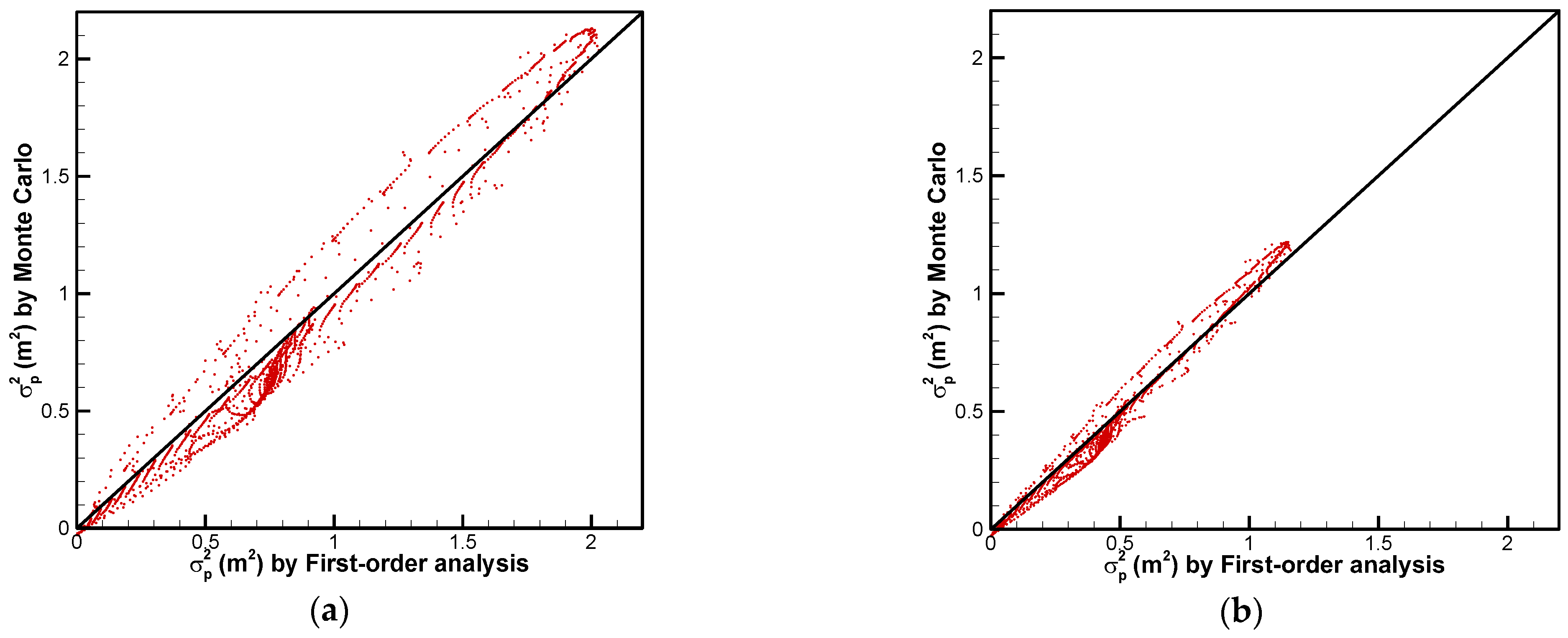
2.3. Monte Carlo Simulation Verification

Despite the enormous computer effort required by a Monte Carlo simulation, this method is still the most widely acceptable method to obtain various statistical properties [1]. In order to verify the accuracy of the first-order analysis method proposed in this study, Monte Carlo simulation was used. For one simulation, a series of realizations of a random field with the same mean (${\mu }_{K_s}$),variance (${\sigma }_{K_s}^2$) and correlation length ($\lambda$) were generated, and the hydraulic response was calculated for each realization. These hydraulic responses (e.g., pressure head) were then used to calculate statistical properties such as mean and variance, which can be compared with the results produced by the first-order analysis. In order to generate a statistically stationary and isotropic random field, the fast Fourier transform code, modified from [23], was applied.

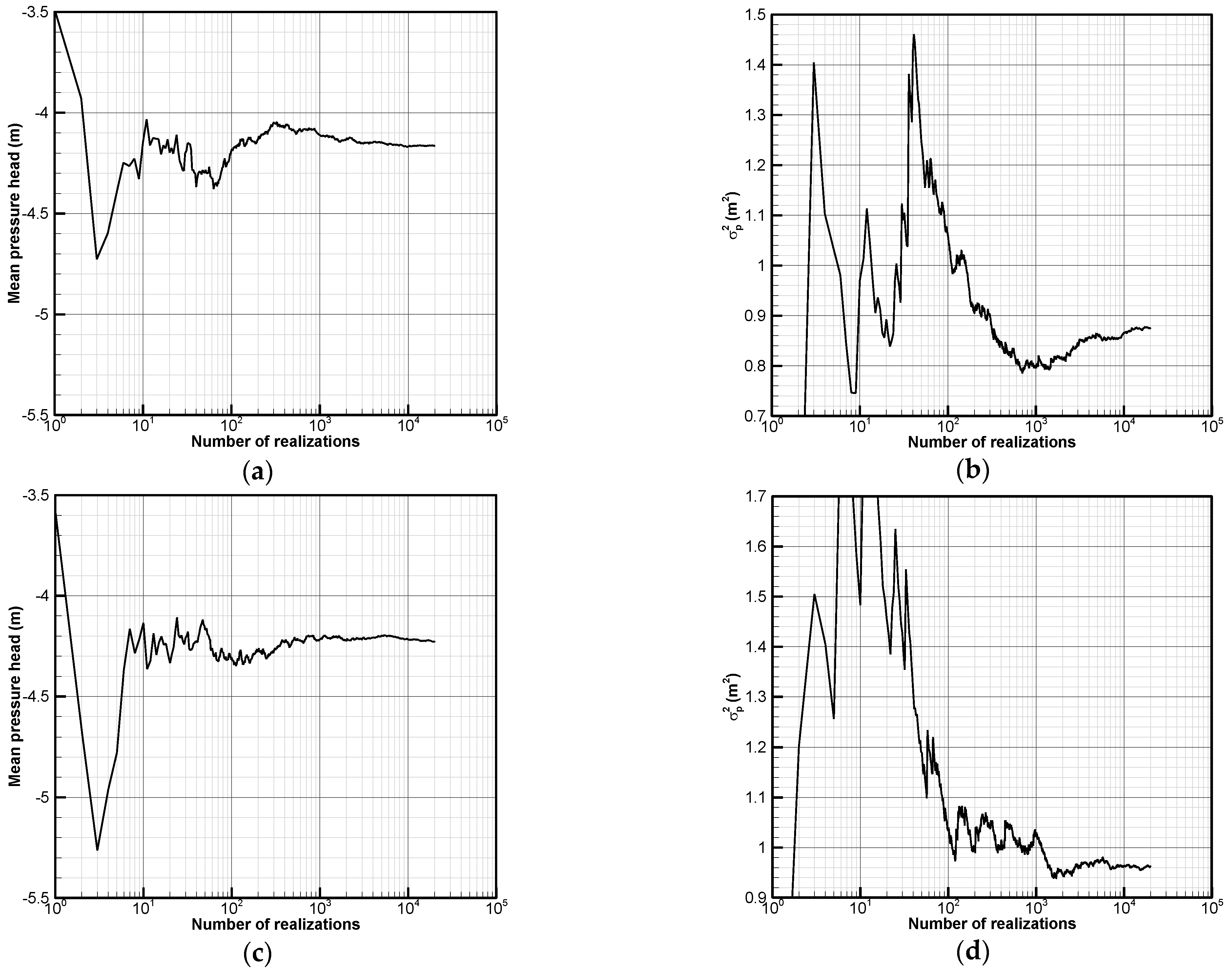
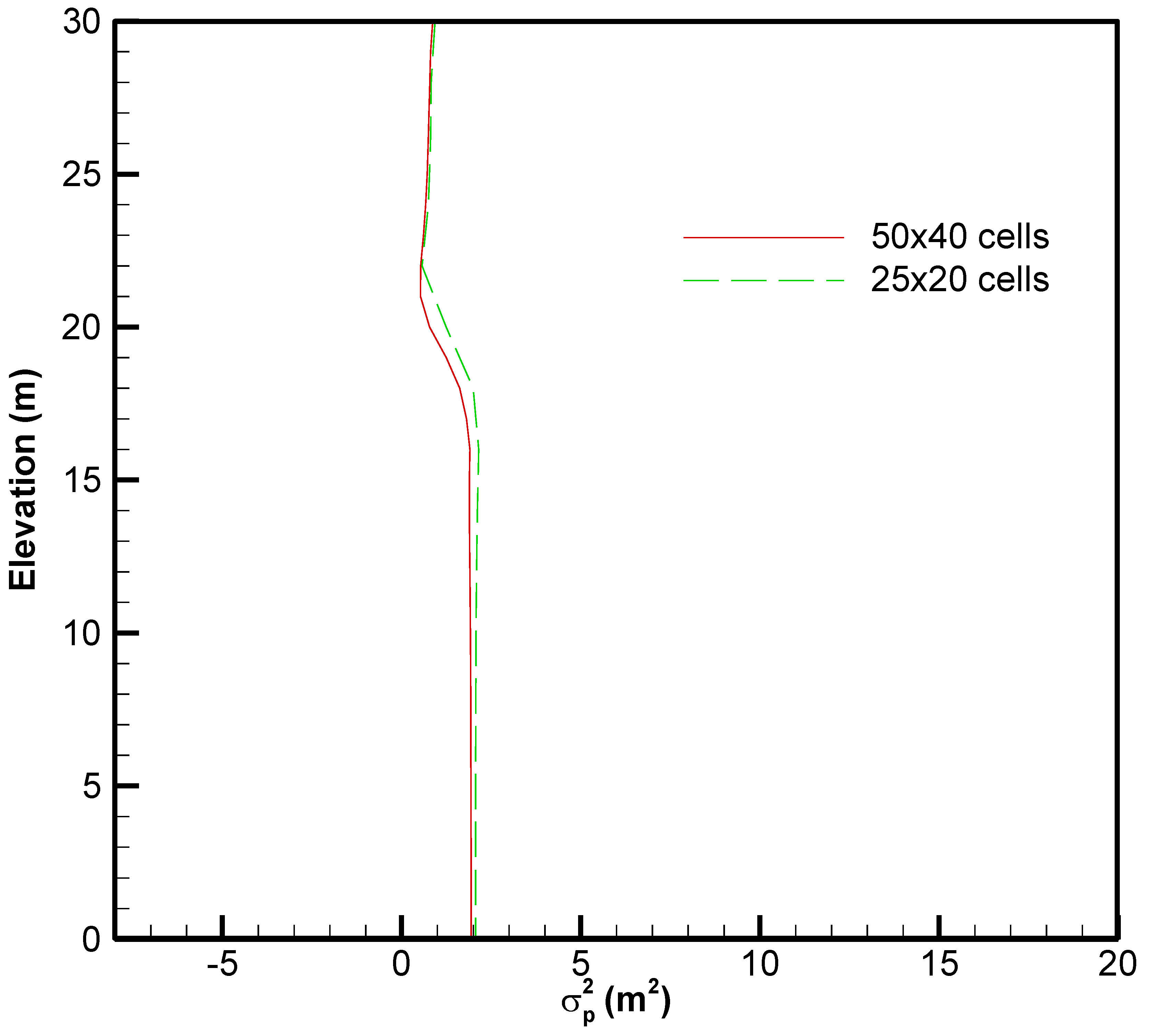
The grid density of the random field, which is crucial in a Monte Carlo simulation, decides the amount of random data appearing in one realization, and hence influences the number of realizations needed to reach convergence. A coarse grid with 25 × 20 cells and a fine grid with 50 × 40 cells of random fields are generated to investigate how the random field grid density affects the number of realizations required for a Monte Carlo simulation. These two sets of grid size have also been applied in the first-order analysis to test the algorithm stability of the first-order analysis approach.

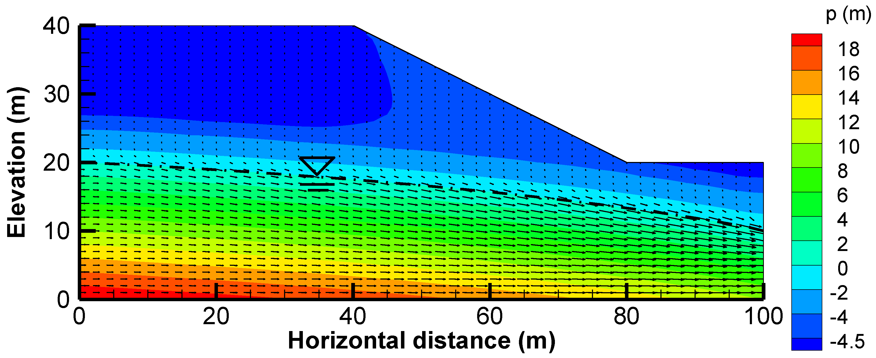
In addition, a single realization of a $K_s\left(x,z\right)$ random field was generated using this fast Fourier transform method with the given mean, variance and correlation length of $K_s\left(x,z\right)$. This random field was then used to simulate the head response within a heterogeneous slope. The response within the heterogeneous slope was subsequently compared to the response derived from mean parameter, ${\mu }_{K_s}$ (homogeneous slope), to show the effect of heterogeneity on the pressure head profile.

2.4. Setup of Simulations

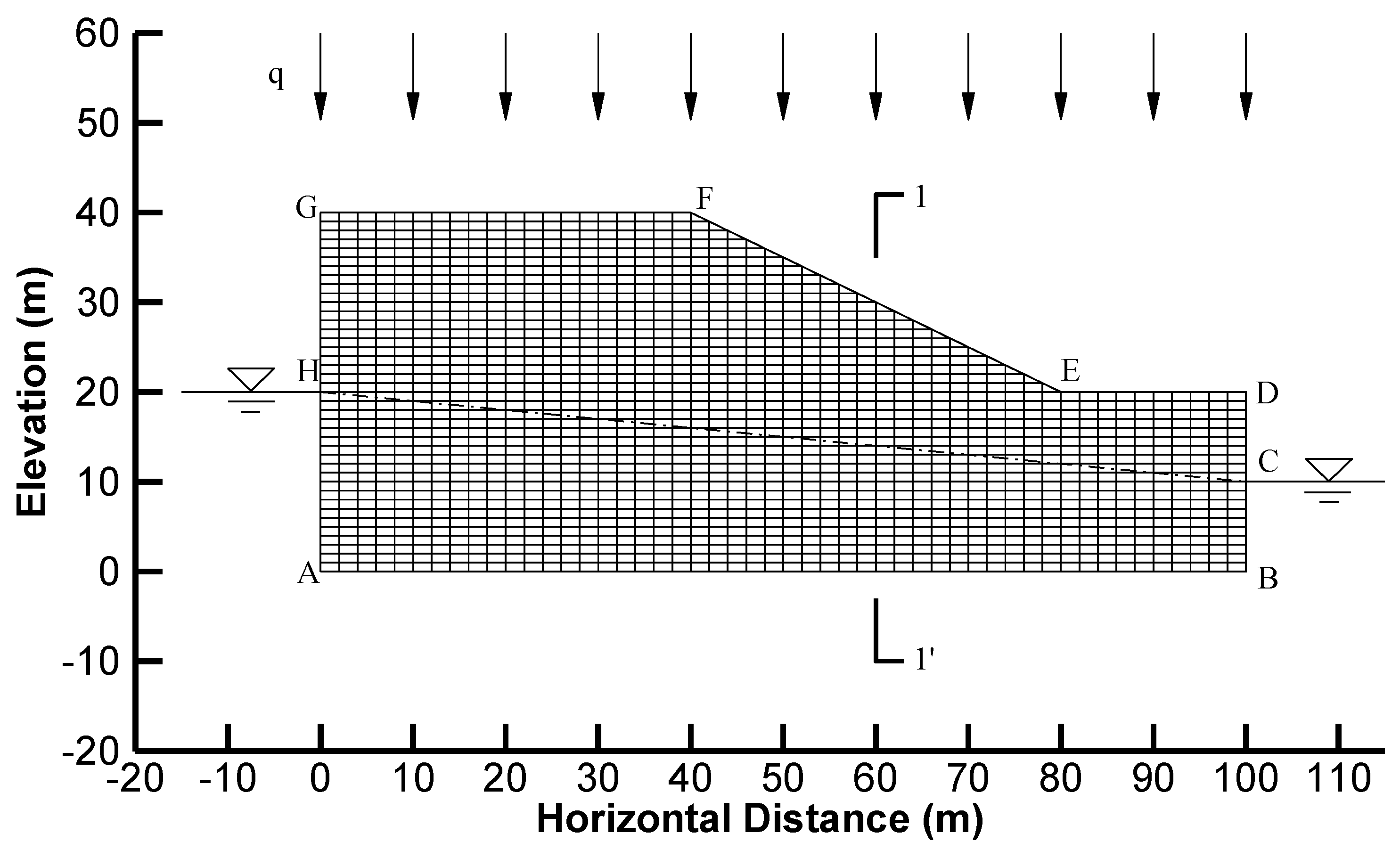
A finite element numerical modeling of the steady seepage flow due to rainfall infiltration was conducted within a 2D hypothetical slope (Figure 2) and was based on a variably saturated flow and transport in 2D (VSAFT2) platform [24]. Firstly, the simulation domain (100 m × 40 m) was evenly discretized into 50 × 40 elements and 2091 nodes. Then, the top right corner of the domain was truncated, and the shape of the remaining part, with 1610 elements and 1681 nodes, was the geometry of the slope (Figure 2). The soil hydraulic parameters used in this study are listed in

Table 1. Soil hydraulic parameters used in the study.

Parameters	Values
Mean of saturated hydraulic conductivity, ${\mu }_{K_s}$	$1.0\mathrm{m}/\mathrm{d}$
Coefficient in MVG model, $\alpha$	$0.4{\mathrm{m}}^{-1}$
Exponent in MVG model, $n$	$2$
Exponent in MVG model, $m$	$0.5$
Residual volumetric water content, ${\theta }_r$	$0.07$
Saturated volumetric water content, ${\theta }_s$	$0.4$
Vertical infiltration flux, $q$	$0.01\mathrm{m}/\mathrm{d}$
Variance of $\ln \left(K_s\right)$, ${\sigma }_{\ln K_s}^2$	$0.4$, $0.7$
Correlation length of $\ln \left(K_s\right)$, $\lambda$	$0.1$, $0.5$, $1$, $10$, $100\mathrm{m}$

. These parameter values are mainly from the study by [25]. Based the published literature [1,5,9,10], the general range of ${\sigma }_{{\ln K}_s}^2$ was suggested to be 0.1~0.7. The correlation length, $\lambda ,$ of $\ln \left(K_s\right)$ was suggested to be 0.025–100 times the slope height [9]. Actually, the slope height, in addition to the grid size and the entire domain size, should be taken into consideration to determine a proper study range for correlation length [26]. Hence, a range of 0.1–100 m of correlation length, $\lambda ,$ was proposed in this study (Table 1). Finally, the ratio between the vertical infiltration flux and ${\mu }_{K_s}$ was set as 0.01 [9].

Figure 2 displays the boundary conditions for this analysis. The boundaries AH and BC remained a constant head, in which ${\left.\left(h+z\right)\right|}_{AH}=20\mathrm{m}$ and ${\left.\left(h+z\right)\right|}_{BC}=10\mathrm{m}$. The boundary AB was impermeable, and the boundary GF had a constant vertical flux $\mathrm{a}\mathrm{p}\mathrm{p}\mathrm{l}\mathrm{i}\mathrm{e}\mathrm{d},q=0.01\mathrm{m}/\mathrm{d}$. The boundaries FE, ED, GH and DC were defined as seepage faces [16].

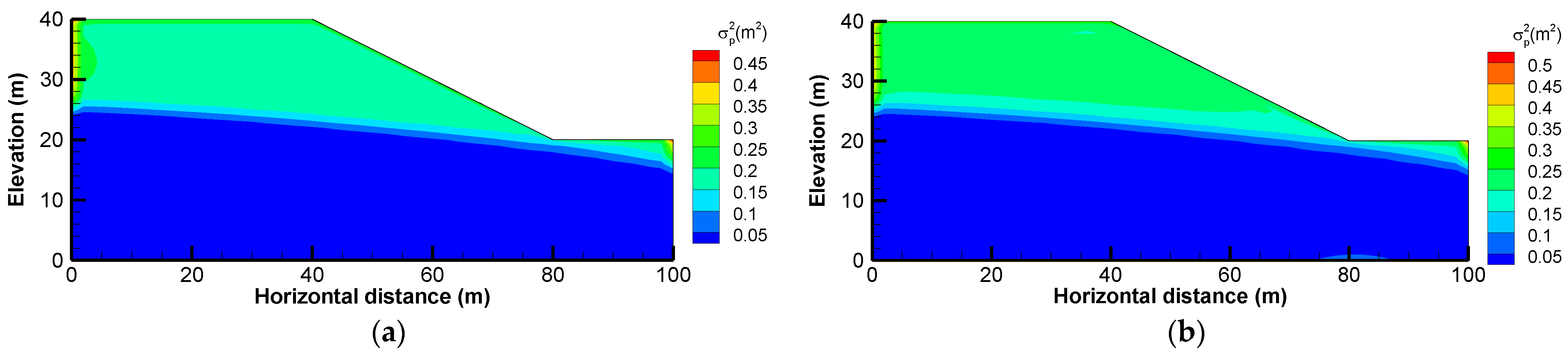
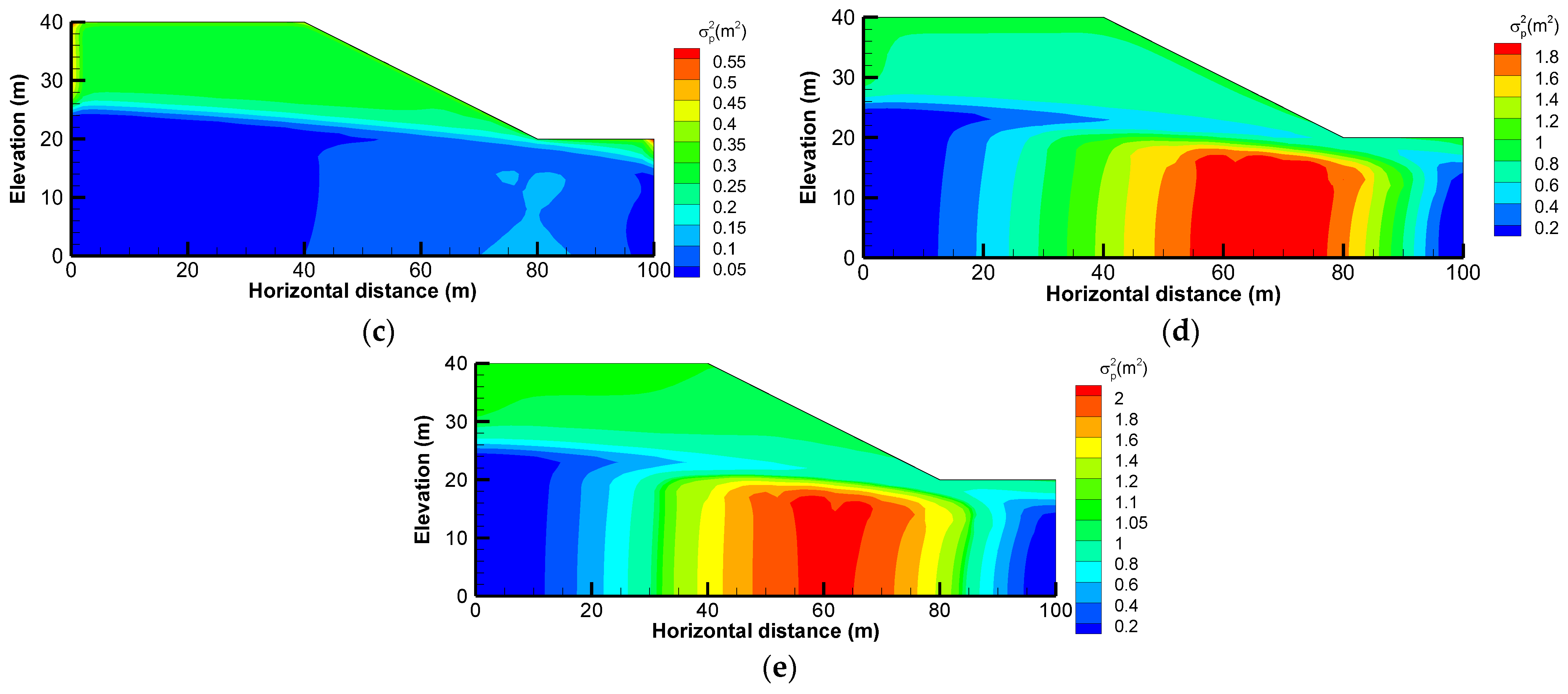
To comprehensively investigate the effect of variability in saturated hydraulic conductivity and to verify the first-order analysis approach proposed, a series of study cases were selected, shown in

Table 2. Statistics of $K_s$ in each study case.

Case No.	${\mathit{\sigma }}_{\mathbf{ln}{\mathit{K}}_{\mathit{s}}}^2$	$\mathit{\lambda }$$\left(\mathit{m}\right)$	Grid	Method
1	0.7	0.1	50 × 40 cells	First-order analysis
2	0.7	0.5	50 × 40 cells	First-order analysis
3	0.7	1	50 × 40 cells	First-order analysis
4	0.7	10	50 × 40 cells	First-order analysis
5	0.7	100	50 × 40 cells	First-order analysis
6	0.7	10	25 × 20 cells	First-order analysis
7	0.4	10	50 × 40 cells	First-order analysis
8	0.7	10	50 × 40 cells	Monte Carlo simulation
9	0.7	10	25 × 20 cells	Monte Carlo simulation
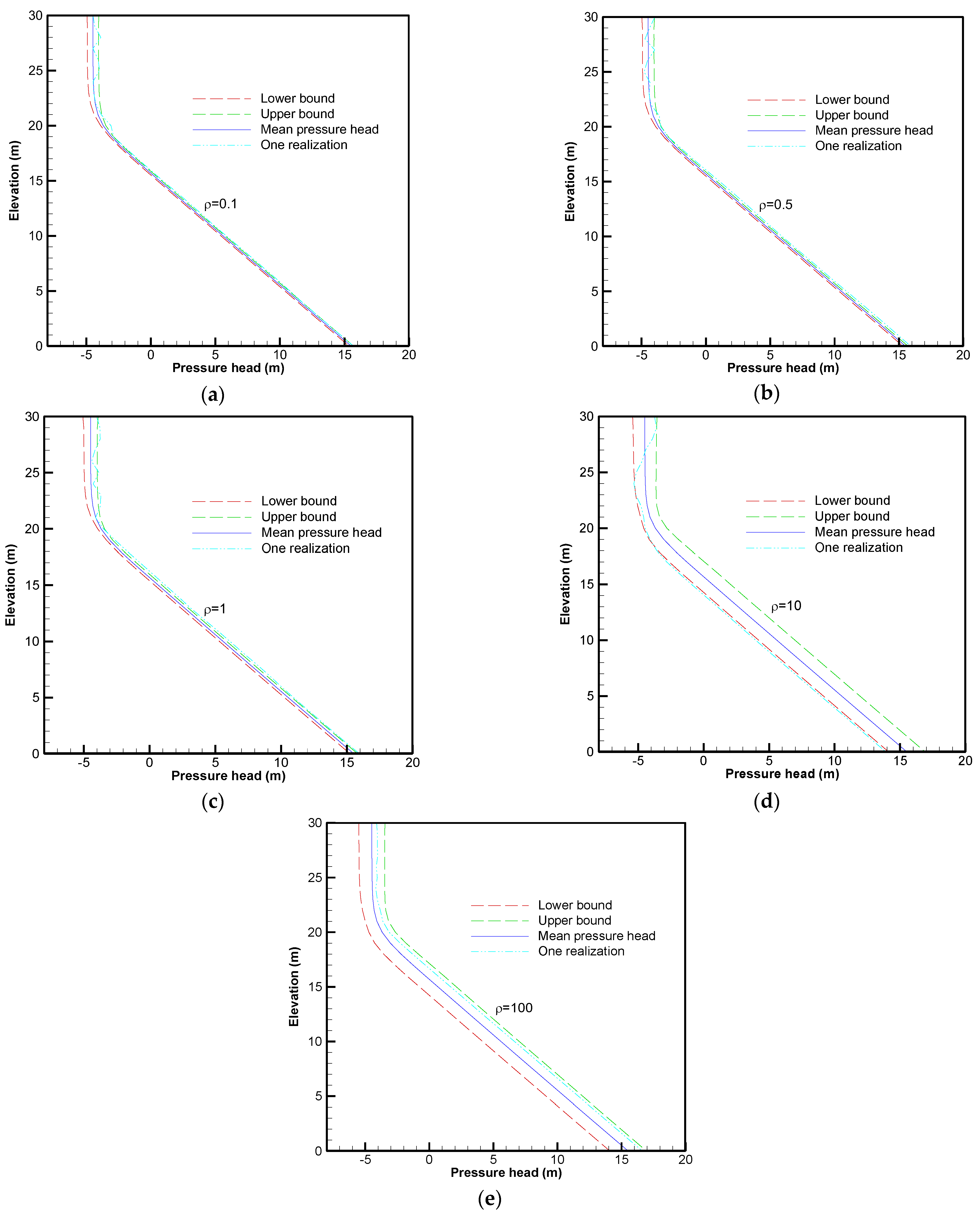
10	0.4	10	50 × 40 cells	Monte Carlo simulation

. From Case 1 to 5, the first-order analysis was carried out to study the variability of the pressure head with respect to the change in the correlation length, $\lambda$, of $\ln K_s\left(x,z\right)$. A single realization of a $K_s\left(x,z\right)$ random field was generated for each $\lambda$ of $K_s\left(x,z\right)$ to calculate the head response within a heterogeneous slope. To use the result of the Monte Carlo simulation as a comparison to verify the accuracy of the first-order analysis method, a, Monte Carlo simulation with two different grid sizes (Case 8 and Case 9) were first conducted to find the number of realizations needed to reach convergence for different grid densities. These two cases with different grid sizes were also applied in the first-order analysis (Case 4 and Case 6). Second, both the Monte Carlo simulation (Case 8 and Case 10) and the first-order analysis (Case 4 and Case 7) were conducted at two ${\sigma }_{{\ln K}_s}^2$ of 0.7 and 0.4.

3. Results and Discussion

The results and discussions are grouped into (1) the effect of the spatial variability of the saturated hydraulic conductivity on the pressure heads and (2) the Monte Carlo simulation verification.

3.1. Effect of Spatial Variability of Saturated Hydraulic Conductivity on Pressure Heads

To reveal the effect of the spatial variability of the saturated hydraulic conductivity on the pressure heads, the deterministic analysis of the mean pressure head with the mean value of the saturated hydraulic conductivity and the first-order analysis of the variance of the pressure head were first conducted. Afterwards, the mean and the variance of the pressure head were used to derive the upper and the lower bounds of the pressure head profile. Finally, these upper and lower bounds served as an appropriate range to discuss the pressure head response within the heterogeneous slope.

3.1.1. Deterministic Analysis

The deterministic analysis was performed assuming the slope was homogeneous, with the mean of the saturated hydraulic conductivity, ${\mu }_{K_s}$, and the soil hydraulic parameters displayed in Table 1. The slope geometry, the grid size and the boundary conditions can be seen in Figure 2. The results, including the vectors of seepage velocity, contours of the pressure head at a steady-state flow and the phreatic surface, of the deterministic analysis are shown in Figure 3. As expected, the rain infiltrates into the slope, merging with the groundwater at the phreatic surface and flowing from high total head to low total head under the phreatic surface. The seepage field derived from the homogeneous, mean hydraulic properties represents the most likely seepage field with given infiltration rates and boundary conditions. Although the most likely seepage field can be quite different from the field based on the heterogeneous hydraulic properties, it shows the general seepage field within the slope. This result presents a basic understanding of seepage within the slope, which demonstrates that VSAFT2 has the ability to predict the infiltration and seepage behavior in an unsaturated slope scenario. The pressure head was calculated can also be used as the mean pressure head in Equation (7).

3.1.2. Pressure Head Variance

For Case 1 to Case 5 in Table 2, the first-order analysis was utilized to calculate the variance of the pressure head at each node in the slope. Analyses were conducted with the same mesh that was used for the deterministic analysis.

Figure 4 shows the variance of the pressure head at each node in the slope. It shows that a higher correlation length leads to a higher variability in the pressure head on the whole. More specifically, the variance of the pressure head above the phreatic surface increases sharply with the correlation length before the correlation length reaches 10 m and then grows slowly until the correlation length reaches 100 m. On the other hand, the increases in the variance of the pressure head below the phreatic surface are mainly around the central part of the phreatic surface.

The amount of different random data of $K_s$ appearing in one realization decreases with the increasing correlation length. Meanwhile, the statistical differences between each generated realization based on the same mean, variance and correlation length increases. To summarize, the amount of random data of $K_s$ appearing in each realization is sufficiently high at small correlation lengths. However, when correlation length becomes larger, each realization generated from the same statistical parameters only contains parts of the random data of the whole probability distribution.

Due to this tendency, the variance of the pressure head is also affected by the boundary conditions. The domain above the phreatic surface is dominated by a constant flux boundary. According to Darcy’s law, the hydraulic gradient is inversely proportional to the $K_s$ field, as is the pressure head. Therefore, at low correlation lengths, the pressure heads do not deviate much from each other due to the similar statistical characteristics of the $K_s$ field. Therefore, the variance of the pressure head is small. However, at large correlation lengths, the pressure head values calculated from different realizations of $K_s$ certainly deviate from each other, and the variance of the pressure head becomes large. This is the reason why the variance of the pressure head is proportional to the correlation length above the phreatic surface.

The domain below the phreatic surface is saturated under the control of a constant hydraulic head difference between ${\left.\left(h+z\right)\right|}_{AH}=20\mathrm{m}$ and ${\left.\left(h+z\right)\right|}_{BC}=10\mathrm{m}$. Using Darcy’s law, the head loss distributes inversely with the $K_s$ distribution along the flow direction, keeping the continuous, specific discharge through the domain below the phreatic surface so that the head distribution is influenced by the discrepancy in the distributions of the $K_s$ field. Therefore, at low correlation lengths, the $K_s$ field of each realization becomes homogenous, in which a relatively high or low zone of $K_s$, which contains many elements, is hardly delineated. Thus, the variance of the pressure head is small. At a relatively high value of correlation length (e.g., 10–100 m in this study), each generated realization has a discrepancy in the distributions of the $K_s$ field. These distributions differ from each other, leading to a large variance of the pressure head. These explanations are supported by the other literature [26,27].

3.1.3. Upper and Lower Bounds of Pressure Head Profile

The standard deviation of the pressure head, ${\sigma }_p,$ derived from Figure 4, is added to and subtracted from the mean pressure head profile obtained from Figure 3 to yield the upper and the lower bounds of the pressure head profile. The pressure head profiles along the cross section 1-1′ (indicated in Figure 2) are shown in Figure 5.

As can be seen from Figure 5, a higher correlation length yields a lower bound with a more negative pressure head and an upper bound with a less negative pressure head. This result is consistent with the findings in the variance of the pressure head shown in Figure 4. However, Figure 5 clearly illustrates that the range of variation of the pressure head can be as much as approximately 3 m due to the uncertainties and spatial variation of the hydraulic conductivity in a slope. In their studies, Santoso et al. [26,27] and Zhu et al. [9] also found that the range of variation of the pressure head changes with the correlation length of the hydraulic conductivity. This can be circumstantial evidence for the effectiveness and accuracy of the first-order analysis.

The fluctuation range of the phreatic surface, which is crucial to the slope stability analysis, can be seen on the left side of Figure 5b where the pressure head is equal to zero. A fluctuation of up to 3 m is shown. More specifically, the fluctuation range of the phreatic surface increases sharply at first when the correlation length value is low. The growth then slows when the correlation length reaches 10 m. The fluctuation range at high correlation lengths is larger than the range at low correlation lengths. This phenomenon is due to the amount of different random data of $K_s$, the boundary condition and the discrepancy in the distributions of $K_s$ field, which has been explained in previous section.

Note that the lower and upper bounds obtained by the first-order analysis are approximate bounds. They delineate the expectation of deviation from the pressure head profile obtained using ${\mu }_{K_s}$ based on a first-order approximation. To summarize, in all possibilities, this fluctuation can be far larger than this expectation: 3 m. Usually, it is suggested that three times the standard deviation, ${\sigma }_p,$ is the range for all the possibilities; this is a fluctuation of 9 m.

3.1.4. Pressure Head Response within Heterogeneous Slope

Figure 6 shows the simulated pressure head profiles at a steady state along Section 1-1′ in the heterogeneous slopes with five different correlation lengths. The corresponding mean pressure head profiles were obtained based on the homogeneous slope assumption, and the upper and lower bounds are associated with the mean pressure head profiles. As can be seen, the pressure head profiles of these heterogeneous slopes differ from the ones based on the homogeneous slope with ${\mu }_{K_s}$ and are bounded by the upper and the lower bounds. These results imply that it is not possible to reproduce the hydraulic response of a real slope under steady rainfall infiltration from any equivalent homogeneous model. The upper and the lower bounds provide an appropriate range to delineate the possible hydraulic response.

The positions of the phreatic surfaces of these heterogeneous slopes also differ from the one based on the homogeneous slope, which can be indicated by the location where the pressure head equals zero in Figure 6a–e. This may also suggest that the shape of the phreatic surface in a heterogeneous slope is different from its shape in an equivalent homogeneous slope.

3.2. Monte Carlo Simulation Verification

For the Monte Carlo simulation verification, we first investigated the influence of the grid density on the probabilistic analysis by both the Monte Carlo simulation and the first-order analysis method. We then compared the results from the first-order analyses with those from the Monte Carlo simulations.

3.2.1. Impacts of the Grid Density

As was previously mentioned in Section 2, the grid density decides the amount of random data appearing in one realization and the number of realizations needed to make the Monte Carlo simulation reach convergence. Changes in the grid density also can be used to test the algorithm stability of the first-order analysis proposed here. For this purpose, a fine grid with 50 × 40 cells and a coarse grid with 25 × 20 cells were adopted for both the Monte Carlo simulation and the first-order analysis.

Figure 7 shows that the mean and variance of the pressure head of Point F (slope top) changes with the number of realizations obtained by the Monte Carlo simulation for Case 8 and Case 9. Both cases involved 20,000 realizations.

As can be seen in Figure 7a,b, the mean pressure head initially fluctuates with a maximum range from −3.5 to −4.7 m. With the increasing number of realizations, the fluctuation of the mean pressure head decreases. Finally, it keeps nearly steady after approximately 3000 realizations. The variance of the pressure head can be observed to reach convergence after 10,000 realizations, with a maximum fluctuation of 0 to 1.46 m². Therefore, the minimum number of realizations needed for Case 8 (a fine grid with 50 × 40 cells of random fields) to reach convergence was 10,000.

The result for the coarse grid with 25 × 20 cells of random fields is shown in Figure 7c,d). The maximum fluctuation of the mean pressure head with the increasing number of realizations is from −3.5 to −5.5 m. The maximum fluctuation for the variance of the pressure head is from 0 to at least 1.7 m²: both are larger and more fluctuating than the corresponding result for the fine grid case. In addition, the mean pressure head still maintains a slight fluctuation when the number of realizations reaches a quite high value, 20,000, indicating that the Monte Carlo simulation with a coarse grid size requires a greater number of realizations to reach convergence than the simulation with a fine grid size. This is for to two reasons: firstly, each realization of a coarser grid contains a lesser amount of random data; it therefore needs more realizations to make the results of the Monte Carlo experience the same amount of random data as in the fine grid case to reach convergence. Secondly, a finite element numerical simulation with a coarse grid size reduces the accuracy of the pressure head prediction, making the mean and variance of the pressure head more fluctuating and uncertain.

Comparisons of Figure 7a–d indicate that the mean pressure heads for cases with both the coarse and fine grid sizes are all approximately −4.2 m. However, the variance of the pressure head values in the coarse grid case is larger than the variance in the fine grid case. Again, this can be attributed to an insufficient amount of random data contained in one realization and the reduced accuracy of the pressure head prediction in the coarse grid case.

In summary, the Monte Carlo simulation can only reach convergence based on a large number of realizations, which is time-consuming and computation-consuming. If the number of realizations is not high enough, the result is unreliable.

As a comparison, Figure 8 shows the variance of the pressure head, ${\sigma }_p^2,$ along section 1-1′, which was obtained by first-order analysis, using two different grid densities: a fine grid with 50 × 40 cells (Case 4) and a coarse grid with 25 × 20 cells (Case 6).

According to Figure 8, the ${\sigma }_p^2$ with the fine grid, denoted by the solid red line, is slightly smaller than that of the coarse grid, which is denoted by the dashed green line. This result is consistent with the result obtained by the Monte Carlo simulation in Figure 7. Moreover, this result indicates that changes in grid density have little impact on the ${\sigma }_p^2$ estimated by the first-order analysis approach, which reveals a good algorithm stability of the first-order analysis approach.

3.2.2. Comparison of First-Order Analysis and Monte Carlo Simulation

Scatter plots of the mean and the variance of the pressure head at two variances of $\ln K_s\left(x\right)$, ${\sigma }_{\ln K_s}^2$ = 0.7 and 0.4, obtained from the Monte Carlo simulation versus the results obtained from the first-order analysis are displayed in Figure 9 and Figure 10. In these scatter plots, a red point is located using the means (in Figure 9) or variances (in Figure 10) of the pressure head, which were calculated by the different methods from the same point in the finite element slope model. The solid black line in these scatter plots represents the reference position for a perfect match. More points approaching this line implies that the differences between the results obtained from these two methods are smaller. The Monte Carlo simulation used in Case 8 and Case 10 contains 20,000 realizations, and the correlation length is 10 m.

As is indicated in Figure 9, for both cases with the variances of $\ln K_s\left(x\right)$ equal 0.7 and 0.4, the mean pressure head values range from −5 to 20 m, and the mean pressure head values obtained by the first-order analysis are close to those achieved by the Monte Carlo simulation.

The variances of the pressure head, ${\sigma }_p^2$, obtained by both methods are less consistent with each other. According to Figure 10a, when ${\sigma }_{\ln K_s}^2$ = 0.7, the range of ${\sigma }_p^2$ from the Monte Carlo simulation is from 0 to 2.1. This is slightly broader than the range from the first-order analysis, which is from 0 to 2. The maximum deviation from the reference line is approximately 0.25, which is small and acceptable. As is shown in Figure 10b, when ${\sigma }_{\ln K_s}^2$ = 0.4, the deviation of points from the reference line is up to 0.1. ${\sigma }_p^2$ ranges from 0 to 1.22 from the Monte Carlo simulation, while its range is narrower, from 0 to 1.15, when obtained using the first-order analysis. This is to be expected because the first-order analysis approach ignores the high-order terms in the Taylor series and therefore results in a smaller value of ${\sigma }_p^2$.

Comparisons of Figure 10a with Figure 10b indicate that the deviation from the reference line and the discrepancy of range of ${\sigma }_p^2$ increase with ${\sigma }_{\ln K_s}^2$. This suggests that the accuracy of the first-order analysis approach with respect to deriving statistics such as the mean and the variance of the slope seepages can be sufficiently high when the correlation length and variance of $\ln K_s\left(x\right)$ are not too large.

4. Conclusions

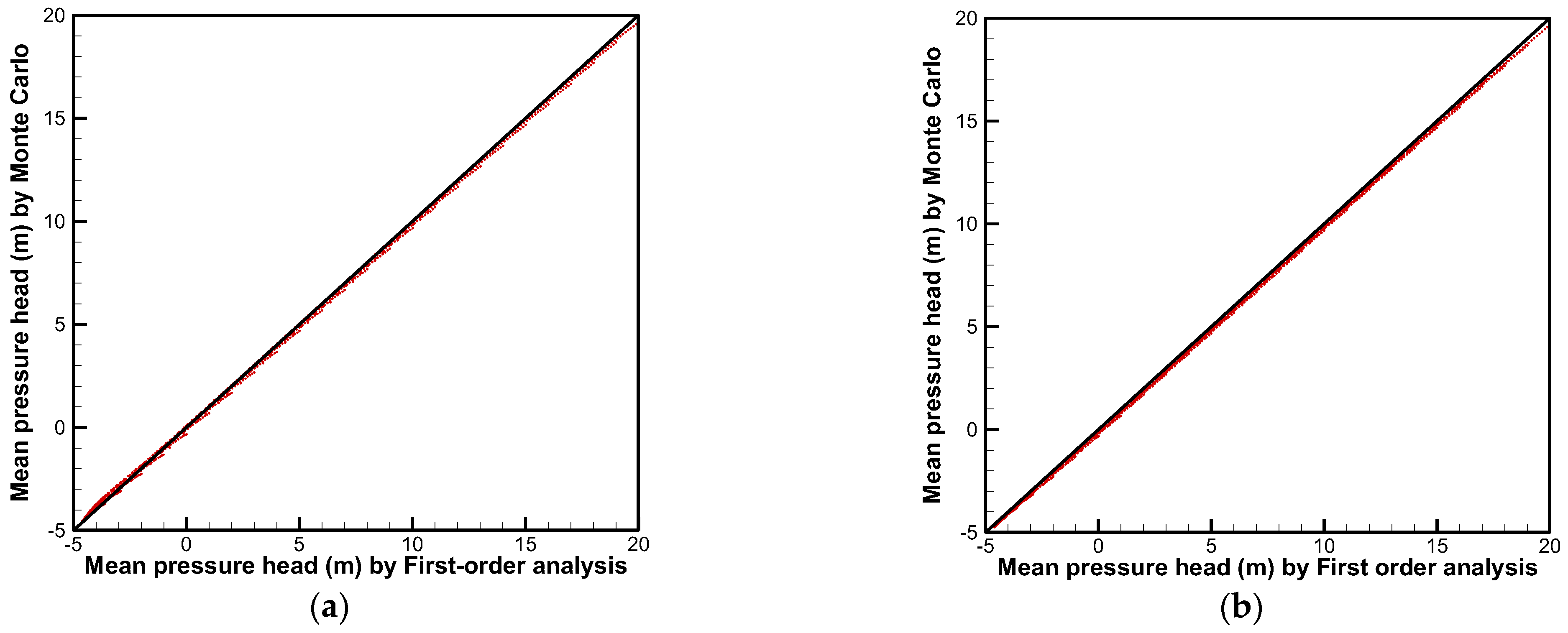
This study conducts a probabilistic analysis of slope seepage under rainfall, considering the spatial variability of hydraulic conductivity. Both the commonly used Monte Carlo simulation method and the proposed first-order stochastic moment approach applied in the probabilistic slope seepage analysis are tested and compared with each other.

Results indicate that the first-order analysis approach is effective and applicable to the study of slope seepage flow. It is capable of obtaining statistics such as mean and variance at a high enough accuracy. With the aid of the first-order analysis approach, it is found that a larger value of the correlation length of $\ln K_s\left(x\right)$ leads to a higher value of the variability in the pressure head and a larger fluctuation of the phreatic surface in the slope. In a heterogeneous slope, the distribution of the pressure head is quite different from that of a homogeneous slope. Therefore, it is not possible to reproduce the hydraulic response of a real heterogeneous slope under steady rainfall infiltration from any equivalent homogeneous model. The upper and the lower bounds obtained from the first-order analysis approach provide an appropriate range to delineate the possible hydraulic response.

The Monte Carlo simulation is found to be time-consuming, requiring at least 10,000 realizations are to reach convergence. In addition, the number of realizations needed is sensitive to the grid density. A coarser grid case needs more realizations for convergence. If the number of realizations is not enough, the result is unreliable. In comparison, the first-order analysis approach reveals a good algorithm stability. The first-order analysis approach is strongly competitive for use in addressing probabilistic slope seepage analysis with fine meshes, especially for the calculation of the sensitivity or the cross-correlation of the pressure head with the hydraulic conductivity, which can be time-consuming and even hard to implement using the Monte Carlo simulation method.

Despite the many advantages of the first-order analysis, it should be emphasized that this approach is based on a first-order approximation. The accuracy of the approximation is generally satisfied when the variance and correlation length of $\ln K_s\left(x\right)$ are not too large. At a large variance and correlation length, a higher order approximation or an iterative approach is proposed (Li and Yeh, 1998), and its application in probabilistic slope seepage analysis may deserve further investigation. Regardless, this study highlights the applicability of the proposed first-order stochastic moment analysis method in the slope scenario.