A Machine Learning Approach for Identification of Low-Head Dams

Abstract

Identifying low-head dams (LHDs) and creating an inventory is a priority, as fatalities continue to occur at these structures. Because obstruction inventories do not specifically identify LHDs and they are not assigned a hazard classification, there is no official inventory of LHDs; a multi-agency taskforce is creating one now by identifying LHDs using Google Earth Pro (GE Pro). The purpose of this paper is to assess whether a machine learning approach can accelerate the creation of the national inventory. We implemented a machine learning approach to use a high-resolution remote sensing data with a Convolutional Neural Network (CNN) architecture. The model achieved 76% accuracy in identifying LHDs (true positives) and 95% accuracy identifying Non-low-head-dams (true negatives) on the validation set. We deployed the trained model for the National Hydrologic Geospatial Fabric (Hydrofabric) flowlines in the Provo River watershed. The results showed a high number of false positives and low accuracy due to the mismatch between Hydrofabric flowlines and actual waterways. We recommend improving the accuracies of the Hydrofabric waterway tracing algorithms to increase the percentage of correctly classified LHDs.

1. Introduction

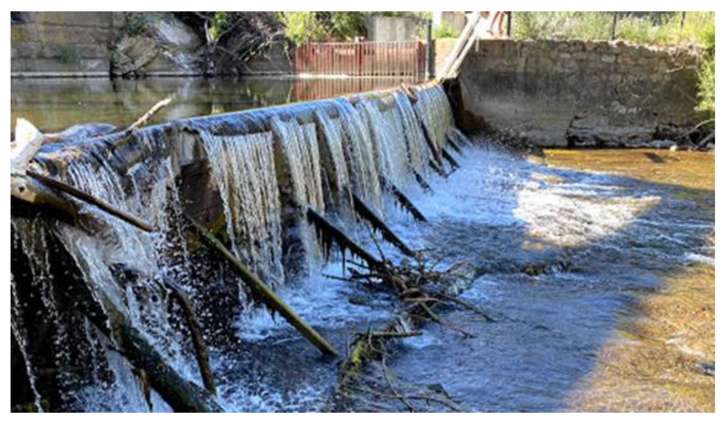
Low-head dams (LHDs; Figure 1), also known as “drowning machines” [1], are defined by the Federal Register [2] as a dam built across a stream, designed to continuously pass flows from upstream to downstream over the entire width of the crest. One of the main purposes of LHDs is to raise the water level upstream to divert water for irrigation and other beneficial uses. 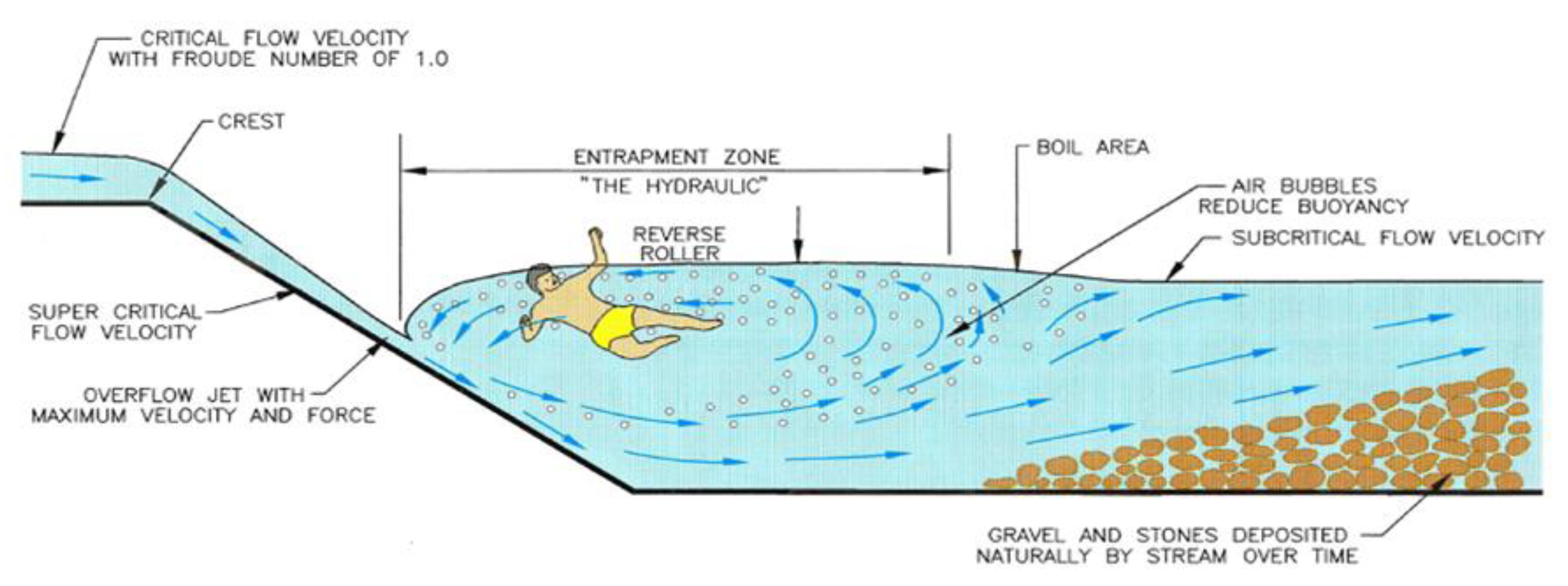LHDs not only affect stream connectivity [3], but, under specific downstream conditions, can create dangerous currents just downstream from the crest, known as a submerged hydraulic jump (SHJ) [4]. A SHJ (Figure 2) will occur when the downstream tailwater depth (TW) is slightly greater than the sequent depth [5]. Submerged hydraulic jumps are responsible for more than a thousand fatalities at LHDs across the United States since 1950. Efforts have been made to create a low-head dam fatality database to raise awareness of their potential dangerous conditions [6].

Edward Kern [6] describes the importance of creating a national inventory of low-head dams to address standards and improve public safety. Similar to Kern [6], Januchowski-Hartley [7] describes the importance of documenting the location of instream obstructions to restore stream connectivity. LHDs are often overlooked by obstruction inventories because they do not have a hazard classification and because they are under 1.8 m high. Most of the United States’ 2.5 million dams are not under the jurisdiction of any public agency, making it difficult to document ownership [8]. Some states explicitly exclude small dams from the definition of an obstruction, stating that “A barrier is not considered a dam if the height does not exceed 1.8 m (6 feet) regardless of storage capacity or if the storage capacity at maximum storage volume does not exceed 18,500 cubic meters (15 acre-feet) regardless of height” [9].

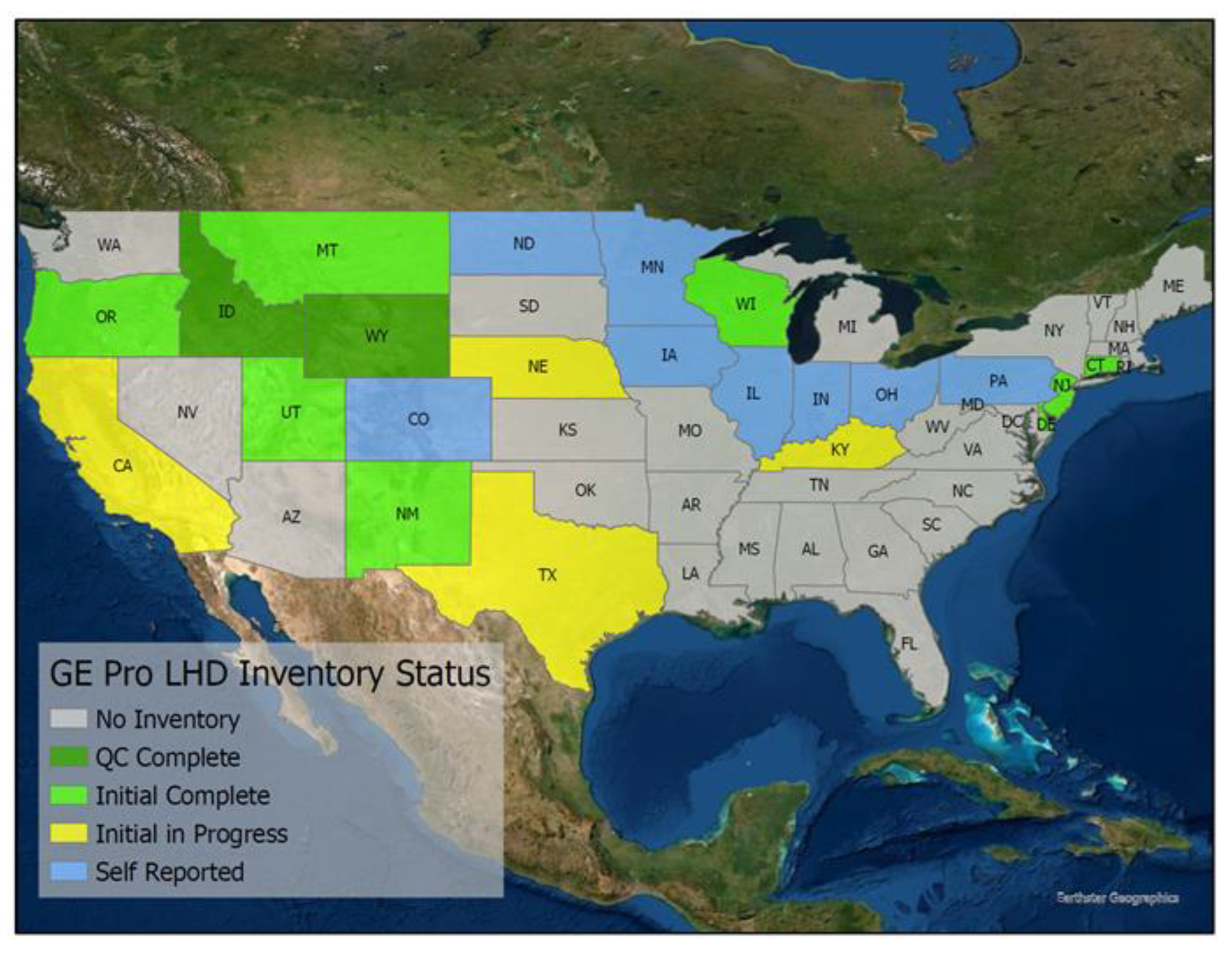
A multi-agency taskforce is creating a national inventory of LHDs [10], focusing its efforts on manual identification using Google Earth Pro (GE Pro). As fatalities continue to occur, more and more private and federal organizations are joining the effort to create the inventory. Figure 3 shows the inventory status, demonstrating that there is more work to be done. Whittemore [11] mentions the great potential of fusing participatory manual efforts for creating instream infrastructure inventories with Machine Learning (ML) approaches that are faster than manual approaches, but require large training and testing datasets. With the increase in data availability and computational power, the interest in ML applications has increased, providing more examples and applications that are useful for this study [12].

The current GE Pro approach is time- and resource-intensive [10]. ML might provide an alternative—and perhaps a faster and more efficient—way to locate LHDs in the United States. The purpose of this paper is to assess whether an ML approach would accelerate the process of creating a national inventory of LHDs.

1.1. Background

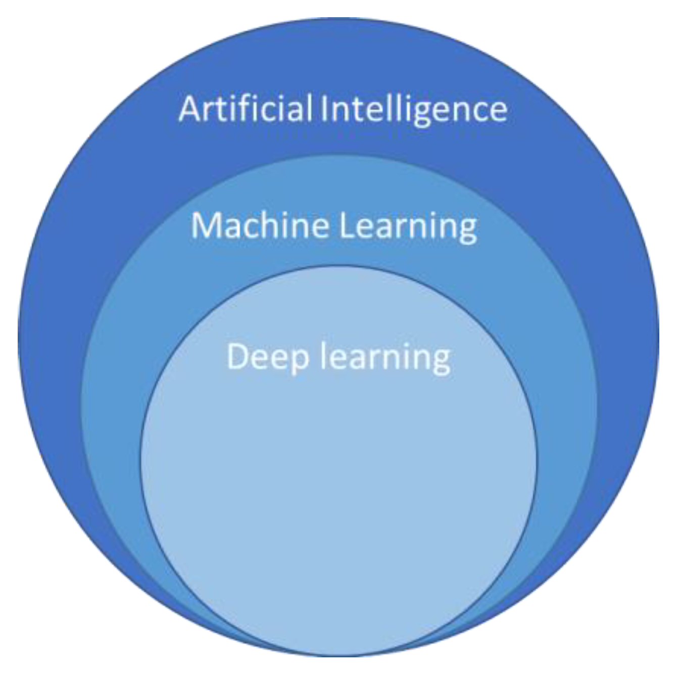
Arthur Samuel [13] defined ML as a “field of study that gives computers the ability to learn without being explicitly programmed”. Deep learning is a type of machine learning (Figure 4) that is based on artificial neural networks and uses multiple layers of processing to identity uniform features within images. Zhang [14] defined it as “the process not only to learn the relation among two or more variables but also the knowledge that governs the relation as well as the knowledge that makes sense of the relation”.

Recent research has shown that Computational Neural Networks (CNN) allow computers to identify and extract features from images, eliminating the task of developing a feature extractor. Deep CNNs have recently substantially improved the state of the art in image classification and other recognition tasks. CNNs were first introduced in the early 1990s, and the availability of larger data sets like ImageNet [15], better models, training algorithms, and the availability of Graphic Processing Units (GPU) are some factors that differentiate them from competing models in image classification [16,17].

Deep CNNs greatly improved with the addition of more training data. When sufficient training data are not available, synthetic transformations of the existing training data can create more data for the training set [16,18].

1.2. Related Work

Recent efforts by Buchanan [19] on automating the process of identification of instream network barriers by using Light Detection and Ranging (LIDAR) DEM 2-meter resolution data and a binary random forest classification algorithm show promising results in identifying unmapped riverine dams. Data used by Buchanan [19] were limited to small areas and are not available nationwide with the same level of spatial resolution, making it difficult to apply that research to a larger scale. Similar work has been done by Swan and Griffin [20] using a fusion of LIDAR and optical remote sensing data to identify and measure impoundments and their dams, showing promising results, but identifying only large dams greater than 5 m high.

Alshehhi [21] suggested the use of high-resolution imagery and a CNN for simultaneous extraction of roads and buildings; the work shows promising results for the creation of road inventories and other large infrastructure. Similar work was performed by Saito [22] using aerial imagery and CNN to predict multichannel images. Both Alshehhi [21] and Saito [22] showed promising results using CNN and remote sensing data for supervised image classification.

Similarly to the multi-agency taskforce GE Pro work, Yang [23] used Google Earth Engine [24] (GEE) and its capability for accessing cloud-based global high-resolution imagery to identify obstructions on rivers with a width greater than or equal to 30 m, with the objective of creating a Global River Obstruction Dataset (GROD). The work by Yang introduces GEE as a powerful tool for accessing high-resolution imagery and the opportunity to scale any ML approach for identifying instream obstructions. Shelestov [25] explored the efficiency of using GEE cloud-based resources to classify multi-temporal satellite imagery with the potential to be applied to a larger scale. Results show good performance on accessing GEE remote sensing data, but demonstrated that it is limited to the employed classifiers, and was outperformed by a neural network-based approach.

2. Methods

The following steps were used in this study: (1) data preparation, (2) creation of training and testing data, (3) model selection, (4) model training, (5) results and metrics, and finally (6) model deployment.

2.1. Data Preparation

The three sources of data used in this study are available nationwide to allow for eventual application to a larger scale: the National Agriculture Imagery Program (NAIP), the Hydrofabric dataset (Hydrofabric), and GE Pro files (.KMZ) provided by the multi-agency taskforce and from the state of Indiana.

The NAIP provides high-resolution imagery with spatial resolution ranging from 0.3 m to 1.0 m acquired during growing season with 4-band (RGBNIR) spectral resolution. One of the main objectives of the NAIP is to make digital orthophotography available to governmental agencies and the public within a year of acquisition. The NAIP is constantly improving the spatial resolution of the nationwide digital orthophotography that is available nationwide [26].

The Hydrofabric is a high-resolution dataset that represents the water drainage network of the United States with features such as rivers, streams and canals [26]. We used the Hydrofabric flowlines (polylines) feature in the preparation of training, testing, and deployment data for our model.

GE Pro files (.KMZ) were provided by the multi-agency taskforce for Utah, Idaho, and Wyoming [10]. The provided data have been quality-controlled by experienced professionals. Additionally, the LHD inventory from Indiana was created by the Indiana Department of Natural Resources (IDNR) and was obtained from: (https://maps.indiana.edu/previewMaps/Infrastructure/Dams_Low_Head_IDNR.html, accessed on 6 September 2022).

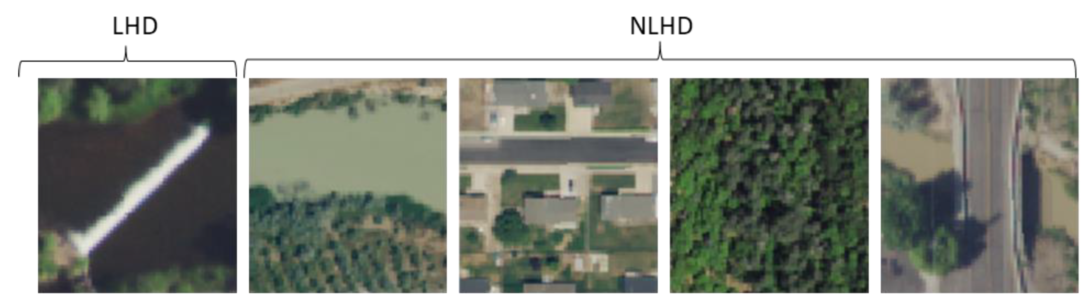
2.2. Creation of Training and Testing Data

We defined two classes for this study: Low-head dams (LHD) and Non-Low-head dams (NLHD) (Figure 5).

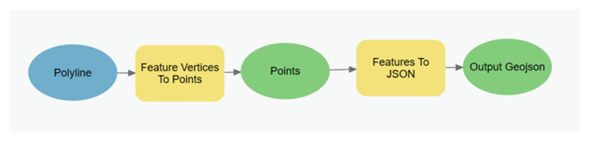
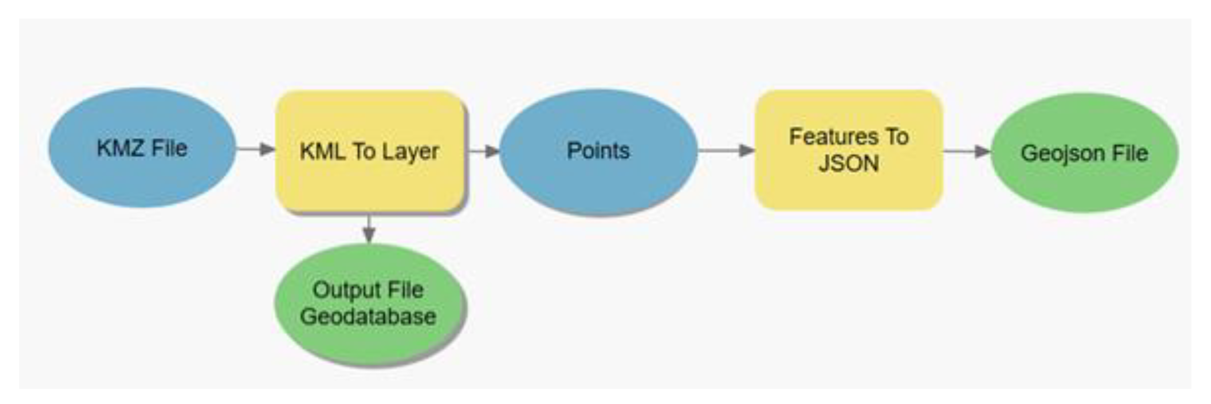
We selected 167 LHD locations for the LHD class testing from the data provided by the multi-agency taskforce and the INDNR that best represented actual LHDs. The dataset was processed with ArcGIS Pro (Figure 6). We adapted a python script that was created by Gorelick [27] that connects with the high-volume GEE Application Programming Interface (API) to extract the LHD image chips from the NAIP image collection.

For the creation of training data belonging to the NLHD class, we analyzed a 5-mile section of the Provo River in Utah to define what our model might encounter as NLHDs: sections of the river without a low-head dam, sections with only vegetation or with bridges, or urban areas. We selected sections of the NHD Plus that represented the features mentioned, and the Utah Department of Transportation inventory of bridges available on the ArcGIS Pro web services. The selected features were processed on ArcGIS Pro (see Figure 6 and Figure 7) and the image chips were extracted with the adapted Gorelick [27] python script.

The characteristics of the image chips include spectral resolution 3 (RGB), dimensions of 128 × 128 pixels with a spatial resolution of 1.0 m, and a .png format.

Because the number of LHD locations available for this study was limited, we dealt with a data imbalance problem: not enough LHD locations. We augmented the LHD data using the following techniques [18] to artificially create training data: rotation range, width shift range, height shift range, zoom range, and horizontal flip. An overview of the datasets is displayed on

Table 1. Overview of the datasets.

Dataset	Training	Testing
Low-head Dam	798	34
Non Low-head Dam	994	34

.

2.3. Model Selection

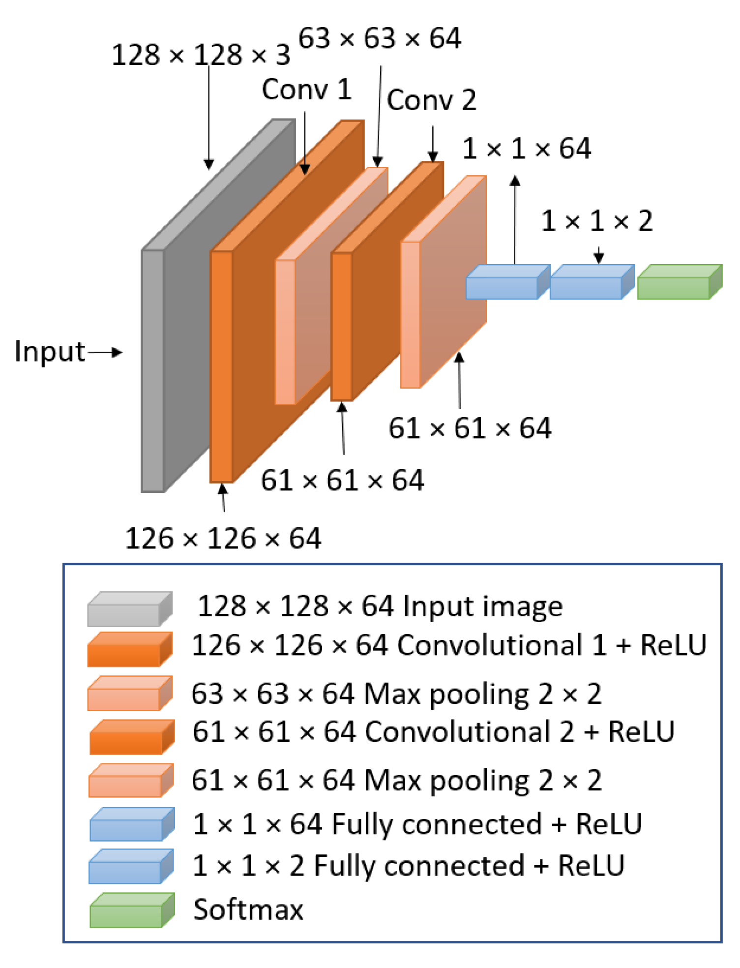
CNNs are considered the most efficient deep learning models for image classification [28]. We employed a binary class prediction method with the use of a single CNN architecture composed of two convolutional layers and two dense layers (Figure 8). We used TensorFlow with keras API to build the CNN model. For the convolutional layers, we used the following hyperparameters: stride with 1 × 1 size and padding as “valid”, which drops the border of the images and makes them smaller from layer to layer, while the “same” padding value would add a border of zeros to keep the image the same size. We also implemented Max Pooling with a pool size of 2 × 2, which helps the CNN to extract high-level features. Because we used padding as valid, the original size of the image reduces from 128 × 128 to 126 × 126. Our feature map changes from layer to layer, but the first feature map is size 126 × 126, and it reduces in size until we have a size 1 × 1 feature map, as shown in Figure 8. We used Rectified Linear Unit [29] (Relu) and SoftMax [30] as activation functions. The Relu activation function is a piecewise linear function that has become a default for several neural networks, because it is easy to implement and achieves better performance when training the model [31]. The SoftMax activation is a mathematical function applied to the last output layer, which converts a vector of numbers into a vector of probabilities to normalize the output into a probability distribution over the predicted output classes.

2.4. Model Training

We trained the CNN model using the training data by setting the epochs to 2000 with early stopping [32] to avoid model overfitting. The early stopping was set up with the monitor set to “validation accuracy”, a patience value of “5”, and restoring best weights to “true”. We used a learning rate of 0.001. The training was performed on a Windows 11 Laptop with Intel Core 9 11th Gen and 16 GB of RAM; no GPU was used for model training. About ten minutes of computer time was required.

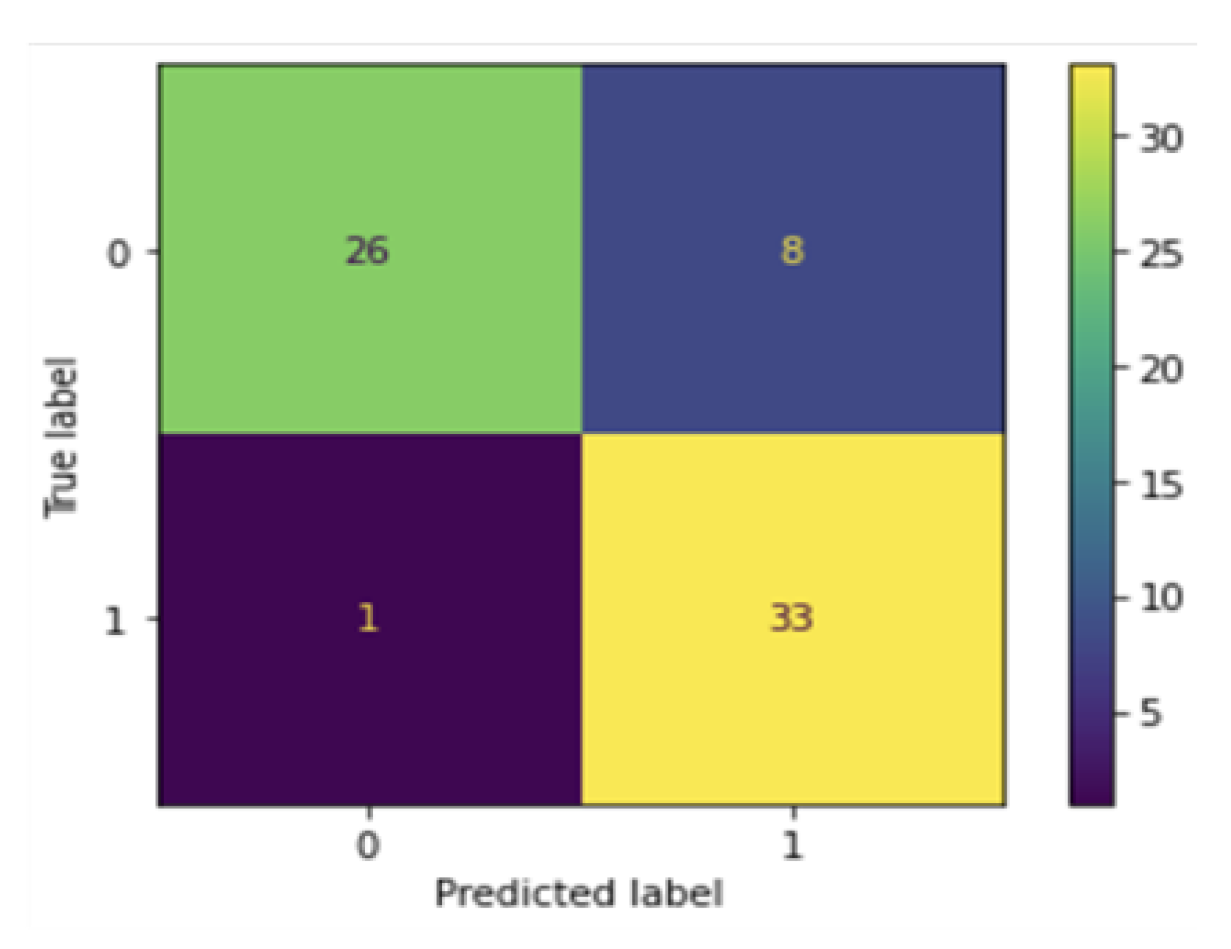
2.5. Confusion Matrix and Metrics

The CNN model was used on the testing data and achieved an accuracy of 76% for classifying LHDs and 95% accuracy classifying NLHDs (see Equation (1) and the confusion matrix in Figure 9).

$$\mathrm{Accuracy}=\frac{\mathrm{True}\mathrm{Positives}}{\mathrm{True}\mathrm{Positives}+\mathrm{False}\mathrm{Positives}}$$

(1)

2.6. Model Deployment

In this section of the paper, we describe the deployment of the trained CNN model for two different areas of interest: Utah County using the Hydrofabric flowlines, and then the Provo River watershed using both the Hydrofabric flowlines and flowlines delineated by hand (hand-delineated).

2.6.1. Deployment of the CNN Model for Utah County

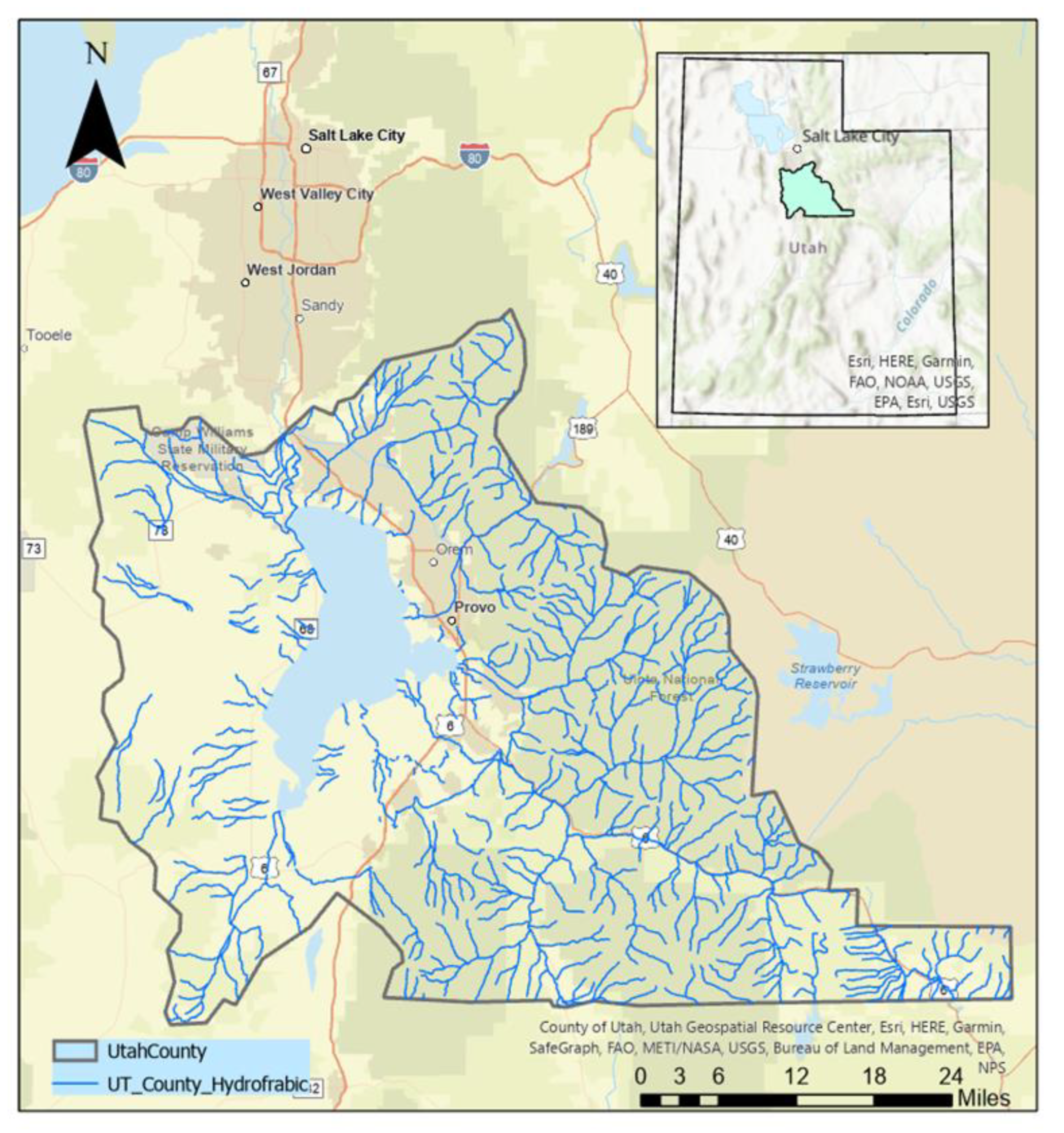
We first deployed the trained CNN model using the Utah County Hydrofabric flowlines (Figure 10) using a stream order of five. The flowlines consist of 182,006 images with 20 known LHD locations. The purpose of this experiment was to assess the accuracy of the trained CNN model when deployed on a larger scale.

2.6.2. Deployment of the CNN Model on Provo River Watershed

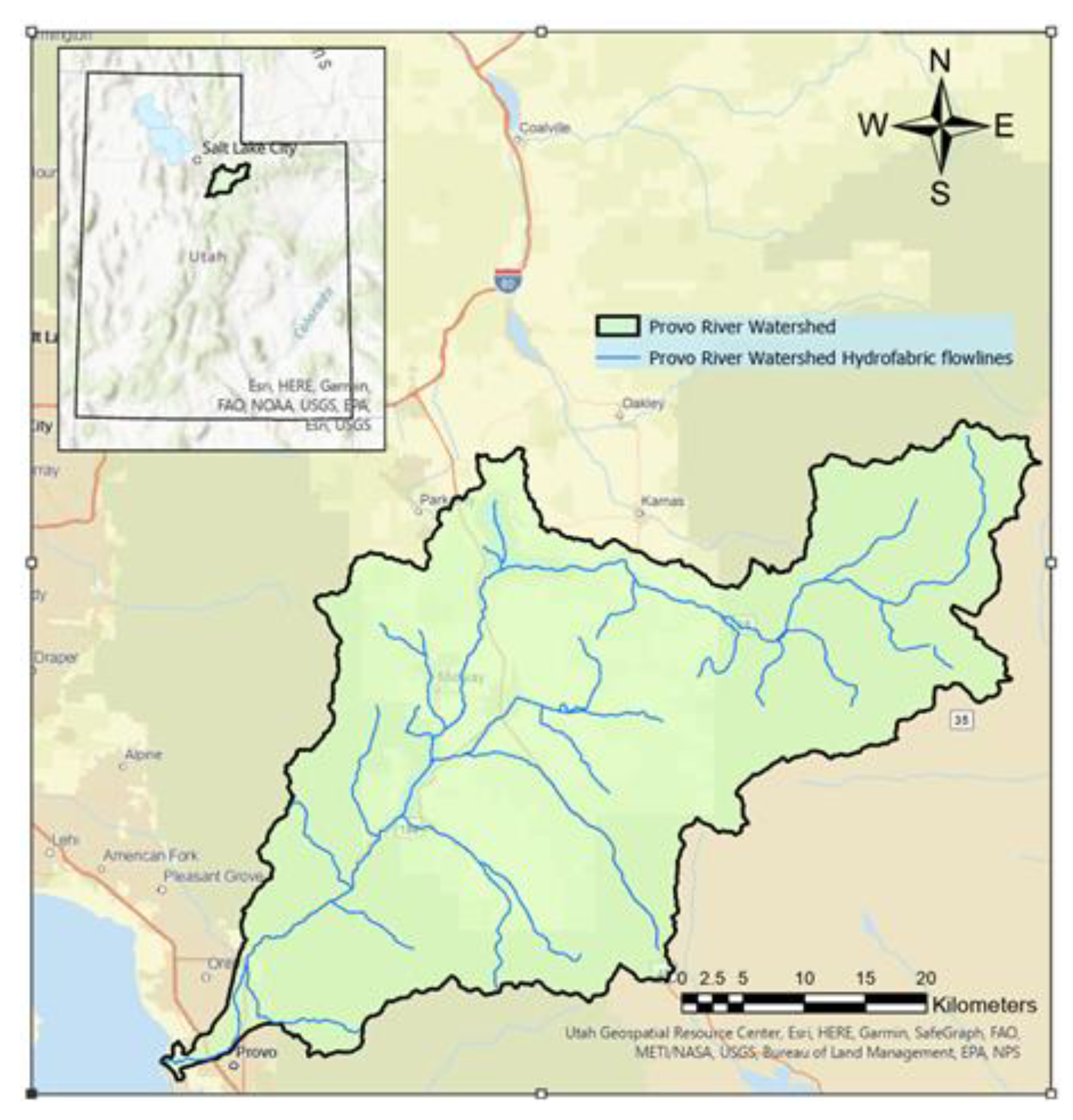
We subsequently deployed the trained CNN model for the Provo River Watershed for two cases. The first used the Hydrofabric flowlines and the second used hand-delineated flowlines (Figure 11). The purpose of this experiment was to deploy the trained CNN model into a smaller domain making possible the hand-delineation of the Provo River watershed flowlines.

3. Results

3.1. Utah County

The trained model was first deployed using the Utah County Hydrofabric flowlines that produced 40,574 image chips. The model classified 615 images as LHDs, correctly identifying 3 of 20 known LHD locations, leaving 612 images as false positives.

3.2. Provo River Watershed

The Provo River watershed Hydrofabric approach resulted in 6156 image chips. The model classified 132 images as LHDs and was able to correctly identify 3 of 21 LHD locations correctly, leaving 129 images as false positives. The Provo River watershed hand-delineated approach resulted in 6008 image chips. The model classified 196 images as LHDs and was able to correctly identify 13 of 21 LHD locations, leaving 183 images as false positives. Results are summarized in

Table 2. Summary of the comparison between the Hydrofabric and the hand-delineated flowlines in the Provo River watershed.

Flowline Type	Number of Images	Actual Number of LHDs	Number of Images Classified as LHDs	Number of LHDs Identified	Number of False Positive
Hydrofabric	6156	21	132	3	129
Hand-delineated	6008	21	196	13	183

.

4. Discussion of Results

4.1. Utah County

Using the Hydrofabric flowlines on the Utah County produced a high number of false positives, leading to the Provo River watershed experiment to determine whether the Hydrofabric flowlines on the high number of false positives and low percentage of correctly classified LHD locations.

4.2. Provo River Watershed

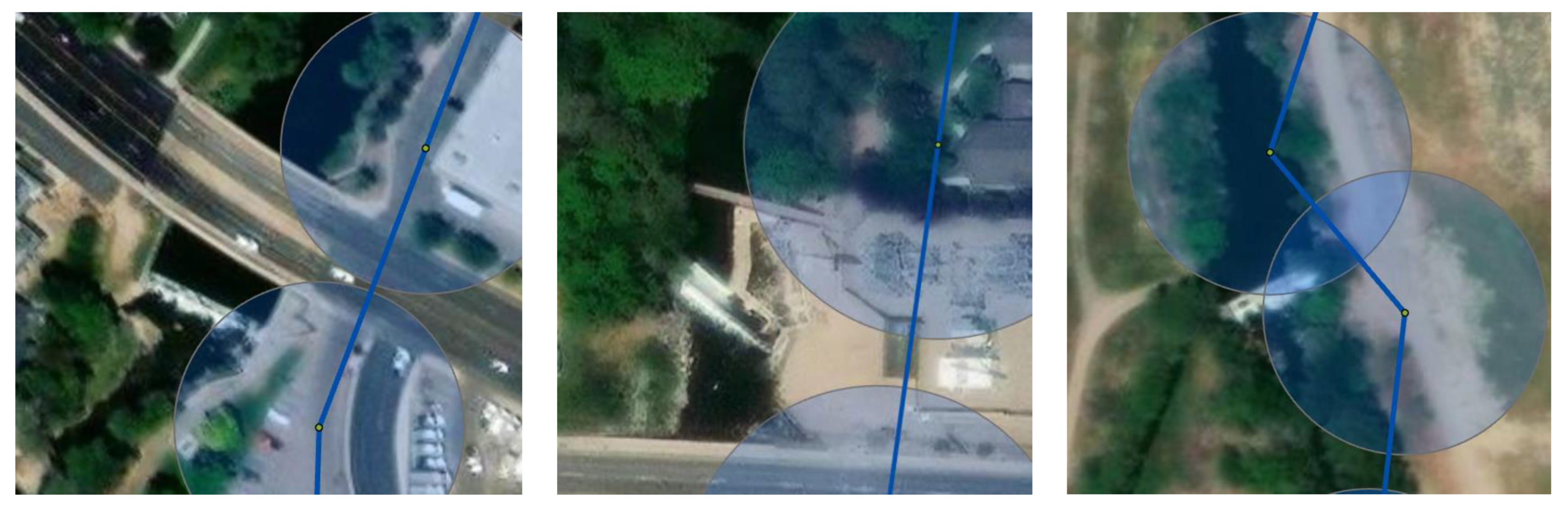
Using the Hydrofabric flowlines for the Provo River watershed produced an unacceptably high number of false positive LHD locations while correctly identifying less than fifteen percent of the actual LHDs. Figure 12 demonstrates that the Hydrofabric flowlines do not always coincide with waterways, and, as shown in the examples, most of the time miss the locations of LHDs.

On the other hand, the deployment of the CNN model using the hand-delineated flowlines showed a reduced number of false positive images while correctly identifying more than half of the actual LHDs. While the percentage of false positives using the hand-delineated flowlines was higher than with the Hydrofabric (3 percent vs. 2.1 percent, respectively), the low number of correctly identified LHDs using the Hydrofabric data makes it impractical as a tool for accelerating the process of finding LHDs. More work with the hand-delineated flowlines during testing will likely increase identification efficiency.

With these results, we were able to identify a major issue with the Hydrofabric flowlines that make the approach untenable for locating low-head dams: unacceptably high numbers of false positives and unacceptably low numbers of correct LHD identifications due to the mismatch between the flowlines and actual waterways.

5. Conclusions/Recommendations

The objective of this paper was to assess whether a ML approach could accelerate the process of creating a national inventory of LHDs. We trained, tested, and deployed a CNN architecture that consisted of two convolutional neural networks and two dense layers. The results of the testing of the model proves that CNN models trained with high-resolution remote sensing data can correctly classify LHDs. On the other hand, the results of the model deployment show that there are challenges that involve the correct identification of LHDs. Some of these challenges are that LHDs can be covered by vegetation, they can be constructed under other structures such as bridges, and they can be constructed on ephemeral streams where water might not have been flowing at the time the image was collected.

After performing the two experiments, we found that because the Hydrofabric flowlines do not always coincide with waterways, a high number of false positives were classified by the model, while a low percentage of actual LHD locations were correctly classified.

We recommend an improved Hydrofabric representation of flowlines, to better match waterways, to increase the percentage of correctly classified LHDs. Additional work may also be conducted to fine-tune the CNN model to achieve the highest accuracy possible. Also, adding more LHDs to the training data and using hand-delineated flowlines, until Hydrofabric accuracy is improved, will increase the accuracy of the CNN model.

References

- Tschantz, B. What we know (and don’t know) about low-head dams. J. Dam. Saf. 2014, 12, 37–43. [Google Scholar]
- Department of Defense. Rules and regulations. Fed. Regist. 2017, 82. [Google Scholar]
- Smith, S.; Meiners, S.; Hastings, R.; Thomas, T.; Colombo, R. Low-head dam impacts on habitat and the functional composition of fish communities. River Res. Appl. 2017, 33, 680–689. [Google Scholar] [CrossRef]
- Leutheusser, H.J.; Fan, J.J. Backward flow velocities of submerged hydraulic jumps. J. Hydraul. Eng. 2001, 127, 514–517. [Google Scholar] [CrossRef]
- McGhin III, R.F.; Hotchkiss, R.H.; Kern, E. Submerged hydraulic jump remediation at low-head dams: Partial width deflector design. J. Hydraul. Eng. 2018, 144, 04018074. [Google Scholar] [CrossRef]
- Kern, E.W.; Hotchkiss, R.H.; Ames, D.P. Introducing a low-head dam fatality database and internet information portal. JAWRA J. Am. Water Resour. Assoc. 2015, 51, 1453–1459. [Google Scholar] [CrossRef]
- Januchowski-Hartley, S.R.; McIntyre, P.B.; Diebel, M.; Doran, P.J.; Infante, D.M.; Joseph, C.; Allan, J.D. Restoring aquatic ecosystem connectivity requires expanding inventories of both dams and road crossings. Front. Ecol. Environ. 2013, 11, 211–217. [Google Scholar] [CrossRef]
- Brewitt, P.K.; Colwyn, C.L. Little dams, big problems: The legal and policy issues of nonjurisdictional dams. Wiley Interdiscip. Rev. Water 2020, 7, e1393. [Google Scholar] [CrossRef]
- Council, S.D.L.R. Rule 74:02:08:01. 2019. Available online: https://sdlegislature.gov/Rules/DisplayRule.aspx?Rule=74:02:08:01 (accessed on 24 August 2021).
- Hotchkiss, R.; Johnson, M.; Crookston, B. Creating a National Inventory of Low-head Dams. In Proceedings of the Dam Safety 2020, Annual Conference of Association of State Dam Safety Officials, Palms Springs, CA, USA, 20–24 September 2020. [Google Scholar]
- Whittemore, A. A participatory science approach to expanding instream infrastructure inventories. Earth’s Future 2020, 8, e2020EF001558. [Google Scholar] [CrossRef]
- Hoeser, T.; Kuenzer, C. Object detection and image segmentation with deep learning on earth observation data: A review-part i: Evolution and recent trends. Remote Sens. 2020, 12, 1667. [Google Scholar] [CrossRef]
- Samuel, A.L. Some studies in machine learning using the game of checkers. II—Recent progress. In Computer Games I.; Springer: New York, NY, USA, 1988; pp. 366–400. [Google Scholar]
- Zhang, W.; Yang, G.; Lin, Y.; Ji, C.; Gupta, M.M. On definition of deep learning. In Proceedings of the 2018 World Automation Congress (WAC), Stevenson, WA, USA, 3–6 June 2018; pp. 1–5. [Google Scholar]
- Deng, J.; Dong, W.; Socher, R.; Li, L.-J.; Li, K.; Fei-Fei, L. Imagenet: A large-scale hierarchical image database. In Proceedings of the 2009 IEEE Conference on Computer Vision and Pattern Recognition, Miami, FL, USA, 20–25 June 2009; pp. 248–255. [Google Scholar]
- Howard, A.G. Some improvements on deep convolutional neural network based image classification. arXiv 2013, arXiv:1312.5402. [Google Scholar]
- Ajit, A.; Acharya, K.; Samanta, A. A review of convolutional neural networks. In Proceedings of the 2020 International Conference on Emerging Trends in Information Technology and Engineering (ic-ETITE), Vellore, India, 24–25 February 2020; pp. 1–5. [Google Scholar]
- Mounsaveng, S.; Laradji, I.; Ben Ayed, I.; Vazquez, D.; Pedersoli, M. Learning data augmentation with online bilevel optimization for image classification. In Proceedings of the IEEE/CVF Winter Conference on Applications of Computer Vision, Virtual, 5–9 January 2021; pp. 1691–1700. [Google Scholar]
- Buchanan, B.P.; Sethi, S.A.; Cuppett, S.; Lung, M.; Jackman, G.; Zarri, L.; Duvall, E.; Dietrich, J.; Sullivan, P.; Dominitz, A. A machine learning approach to identify barriers in stream networks demonstrates high prevalence of unmapped riverine dams. J. Environ. Manag. 2022, 302, 113952. [Google Scholar] [CrossRef] [PubMed]
- Swan, B.; Griffin, R. A LiDAR–optical data fusion approach for identifying and measuring small stream impoundments and dams. Trans. GIS 2020, 24, 174–188. [Google Scholar] [CrossRef]
- Alshehhi, R.; Marpu, P.R.; Woon, W.L.; Dalla Mura, M. Simultaneous extraction of roads and buildings in remote sensing imagery with convolutional neural networks. ISPRS J. Photogramm. Remote Sens. 2017, 130, 139–149. [Google Scholar] [CrossRef]
- Saito, S.; Yamashita, T.; Aoki, Y. Multiple object extraction from aerial imagery with convolutional neural networks. J. Imaging Sci. Technol. 2016, 60, 010402. [Google Scholar] [CrossRef]
- Yang, X.; Pavelsky, T.M.; Ross, M.R.; Januchowski-Hartley, S.R.; Dolan, W.; Altenau, E.H.; Belanger, M.; Byron, D.; Durand, M.; Van Dusen, I. Mapping flow-obstructing structures on global rivers. Water Resour. Res. 2022, 58, e2021WR030386. [Google Scholar] [CrossRef]
- Gorelick, N.; Hancher, M.; Dixon, M.; Ilyushchenko, S.; Thau, D.; Moore, R. Google Earth Engine: Planetary-scale geospatial analysis for everyone. Remote Sens. Environ. 2017, 202, 18–27. [Google Scholar] [CrossRef]
- Shelestov, A.; Lavreniuk, M.; Kussul, N.; Novikov, A.; Skakun, S. Exploring Google Earth Engine platform for big data processing: Classification of multi-temporal satellite imagery for crop mapping. Front. Earth Sci. 2017, 5, 17. [Google Scholar] [CrossRef]
- Partners, O. NAIP Digital Ortho Photo Image. Available online: https://www.fisheries.noaa.gov/inport/item/49508 (accessed on 18 January 2022).
- Gorelick, N. Fast(er) Downloads. Available online: https://gist.github.com/gorelick-google/4c015b79119ef85313b8bef6d654e2d9 (accessed on 18 January 2022).
- Jmour, N.; Zayen, S.; Abdelkrim, A. Convolutional neural networks for image classification. In Proceedings of the 2018 International Conference on Advanced Systems and Electric Technologies (IC_ASET), Hammamet, Tunisia, 22–25 March 2018; pp. 397–402. [Google Scholar]
- Agarap, A.F. Deep learning using rectified linear units (relu). arXiv 2018, arXiv:1803.08375. [Google Scholar]
- Bengio, Y. Learning deep architectures for AI. Found. Trends Mach. Learn. 2009, 2, 1–127. [Google Scholar] [CrossRef]
- Ide, H.; Kurita, T. Improvement of learning for CNN with ReLU activation by sparse regularization. In Proceedings of the 2017 International Joint Conference on Neural Networks (IJCNN), Anchorage, AK, USA, 14–19 May 2017; pp. 2684–2691. [Google Scholar]
- Ying, X. An overview of overfitting and its solutions. J. Phys. Conf. Ser. 2019, 1168, 022022. [Google Scholar] [CrossRef]