Article

Integration of Hydrate-Based Desalination (HBD) into Multistage Flash (MSF) Desalination as a Precursor: An Alternative Solution to Enhance MSF Performance and Distillate Production

1
School of Computing, Engineering and Digital Technologies, Teesside University, Middlesbrough TS1 3BA, UK
2
Centre of Excellence in Desalination Technology, King Abdulaziz University, P.O. Box 80200, Jeddah 21589, Saudi Arabia
3
Department of Mechanical Engineering, King Abdulaziz University, P.O. Box 80204, Jeddah 21589, Saudi Arabia
*
Author to whom correspondence should be addressed.
Water 2023, 15(3), 596; https://doi.org/10.3390/w15030596
Submission received: 2 January 2023 / Revised: 25 January 2023 / Accepted: 27 January 2023 / Published: 2 February 2023
(This article belongs to the Section Wastewater Treatment and Reuse)

Abstract

:
This study considers the integration of multistage flash (MSF) desalination with hydrate-based desalination (HBD) precursor to improve MSF performance in terms of distillate production, longevity, and operational conditions. This is accomplished by a comprehensive analysis of the rate of scale formation, distillate production, and the MSF performance ratio by means of mathematical modelling conducted in Simulink software. To calibrate the effectiveness of HBD as precursor to the MSF desalination process, two MSF models were created: the once-through (OT) and brine recycle (BR) configurations. The MSF models were validated in terms of stagewise distillate production, brine temperature, and coolant temperatures with data from the literature, while neglecting the non-equilibrium allowance. The operational performance of the proposed integration approach was evaluated in terms of the deposition rates of CaCO3, scale thickness, fouling resistance, overall heat transfer coefficient, performance ratio, and production ratio. The examination was conducted from the perspective of water salinity and stream temperature for the integrated HBD-MSF systems. The results show that due to the quality of output water in terms of salinity and temperature, the integration of HBD and MSF improved the performance of MSF by substantially reducing scale formation rates as well as increasing the production of distillate where the scale formation rates were 40.6% and 36.3% lower for the hybrid HBD-MSF-OT and HBD-MSF-BR systems, respectively.

1. Introduction

Multistage flash distillation plants produce about 34% of all desalinated water in the world [1]. Therefore, the improvement of their longevity and efficiency is a very important issue so as to maintain the cost of water at an acceptable level. Scale formation from the precipitation of salts from saline water at heightened temperatures is a universal issue for all major thermal desalination processes around the globe and especially in thermal desalination processes, such as MSF and multi-effect desalination (MED), which operate at higher temperatures. Depending upon the pH requirements for scale formation, scales are often classified as alkaline and non-alkaline scales [2]. The most common forms of alkaline scale consist of CaCO3 and Mg (OH)2. Calcium carbonate-based scale formation is considered to be the most common type of scale that occurs at temperatures as low as 45 °C, whereas magnesium hydroxide-based scale formation occurs at temperatures above 75 °C, which is commonly found in MSF desalination systems that can operate at maximum brine temperatures above 108 °C [3,4,5]. Amongst the non-alkaline forms, the CaSO4 scale has been found to be most common. Like Mg (OH)2, CaSO4 requires temperatures as high as 75 °C to form. As explained by Al-Sofi [2], the precipitation of CaSO4 in any form in MSF plants has been observed only when the plant operates at a temperature above 120 °C.
On the other hand, the trigger for the formation of alkaline scale, e.g., CaCO3, is the lower solubility of salts as well as the accelerated decomposition hydrolysis of seawater bicarbonate ions in solutions at higher temperatures. Consequently, the control of pH would be important in suppressing alkaline scale formation where it was suggested that, by adding inorganic strong acids such as sulfuric acid into seawater, the bicarbonate ions can be depleted [5]. In the same way, various chemical and physical solutions were applied in order to address the problem of MSF scale formation [6]. In addition, various commercial anti-scalants derived from condensed polyelectrolytes, polyphosphates, and organ phosphonates are also widely used in industry [7]. The chemical prevention of scale formation techniques is often associated with challenges such as improper dosage, unsustainability, and instability. Hence, numerous alternatives have been proposed and are in use, such as mechanical cleaning either offline (brushing) or online (using balls) or by employing water flushing or hosing or controlled mechanical vibration [8,9,10,11]. However, these cleaning methods are labour-intensive [12], and other alternatives involve pre-treatment processes. The present study focusses on how pre-treated water from a hydrate-based desalination process could improve multistage flash desalination by improving the operational conditions such as temperature and water salinity. It is worth mentioning that, due to the pre-treatment of feed brine in this study, the system operates at temperatures lower than the 90 °C top brine temperature, and hence, only CaCO3 scale formation is assumed to occur.

2. Methodology

The current study focuses exclusively on the performance of MSF with the feed being either seawater (MSF only system) or the pre-treated water through hydrate-based desalination (HBD-MSF hybrid system). To analyse the performance of the HBD-MSF hybrid process, a mathematical model was developed in Simulink software. For that purpose, two basic steady-state MSF models were created representing once-through (OT) and brine recycle (BR) configurations. These models were created using the configurations presented in the modelling studies of Rosso [13] and Ali and Kairouani [14] and validated. Scale formation then was introduced to the validated model. The results of the model were analysed and compared in the two MSF processes mentioned above before introducing HBD into the process. To model the HBD-MSF process, it is assumed that the water inlet of the MSF model is partially desalinated due to undergoing the hydrate process before arriving at the MSF plant. Consequently, the inlet water would consist of lower levels of salts at a lower temperature. The impact of using partially treated water with 74.5% less salinity resulted from the hydrate process on the total performance of MSF desalination was investigated through simulation and comparison of the results with the two original MSF models in this study. The salt removal efficiency was measured through water conductivity tests upon the dissociated hydrate slurry, where hydrates were generated using an apparatus explained in a study by Thoutam et al. [15]. Details of the modelling are described next.

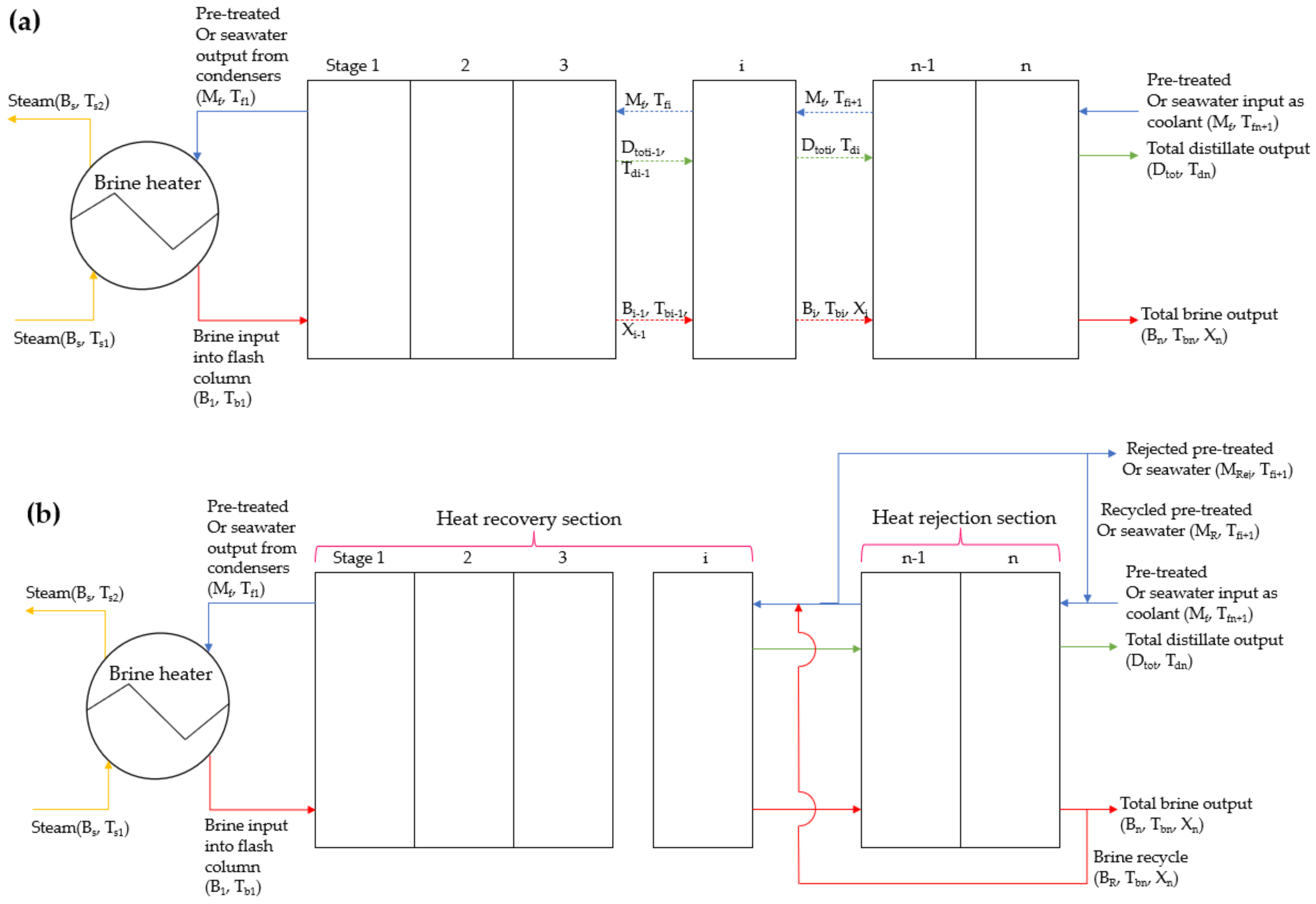
2.1. Multistage Flash Modelling

The following assumptions were made in modelling the MSF desalination column illustrated in Figure 1:
  • Heat losses are negligible apart from the condenser tubes.
  • The distillate produced from the MSF desalination is free of salt.
  • Heat from mixing is negligible.
  • Salinity changes in the coolant flowing in the condenser tubes are negligible
The entire set of modelling equations are a collection of mass and heat transfer equations that are given as follows:

2.1.1. Applied Equations within the Stages

The mass, salt, and energy balances within the flash chamber are given in Equations (1)–(3), respectively:
B i 1 = B i + D i
X b i 1 B i 1 = X b i B i
D i λ v i = B i 1 C p b i 1 T b i 1 T b i
The vapour temperature above the demister does not stay constant since the vapour loses a fraction of heat while passing through it, the correlation for which has been provided by Rosso [13] as:
T d i = T v i e x p   1.885 0.02063 T v i   1.8
The temperature of vapour before passing through the demister would be equal to the brine temperature (Tbi) leaving the stage. The operational pressure (mmHg) of each stage was calculated from the Antoine Equation presented below [16]:
l o g 10 P = A B T + C
where temperature T is in Celsius, and the values of A, B, and C are 8.07131, 1730.63, and 133.426, respectively.

2.1.2. Applied Equations within the Condensers

The heat transfer between the coolant within the condenser and the vapour in the heat recovery section is given in Equation (6):
M R + M f C p f i T f i T f i + 1 = U c i A c ( L M T D ) c i
The values of Log mean temperature difference in Co (LMTD) were calculated from Equation (7):
( L M T D ) c i = T f j T f j + 1 / l n T d j T f j + 1 T d j T f j
Equation (8) was derived to calculate the value of Tf, which was obtained by solving Equations (6) and (7):
T f i = T d i T d i T f i + 1 e U c A c M R + M f C p f j
The overall heat transfer coefficient equation was taken from the MSF modelling work carried out by Alasfour and Abdulrahim [17] as given in Equation (9):
1 U c i = d o d i 1 h i n   i + d o d i r f i + d o 2 k t u b e l n d o d i + 1 h o u t   i + r f o
The parameter hin i can be calculated using the Dittus–Boelter equation [18,19], which is provided in Equation (10):
h i n   i = ( 3293.5 + T f i + 1 84.24 0.1714 T f i + 1 X i f 8.471 + 0.1161 X i f + 0.2716 T f i + 1 d i 0.017272 0.2 0.656 V e l 0.8   d i d 0
The medium of heat transfer coefficient on the outside of the tubes (hout i) is mainly caused by the availability of non-condensable gases (NCGs). In order to maintain the model’s simplicity, the contribution of non-condensable gases towards the heat transfer coefficient is ignored in this study.
The overall energy balance around the condensers in the heat rejection section can be calculated using Equation (11):
D i λ c i + C p d i 1 T d i 1 T d j k = 1 j 1 D k = M c w + M f C p f i T f i T f i + 1
where the subscript k represents any stage number that is less than the ith stage. The heat transfer equation for the condenser tubes in the heat rejection section can be written as shown in Equation (12):
M C R + M f C p f i T f i T f i + 1 = U c i A c ( L M T D ) c i
The temperature of the effluent stream from the coolant from stage i in the heat rejection section can be calculated from Equation (13):
T f i = T d i T d i T f i + 1 e U c A c M C R + M f C p f j
The energy balance around the condensation chamber of the heat rejection section is given in Equation (14):
D i λ c i + C p d i 1 T d i 1 T d j k = 1 j 1 D k = M C R + M f C p f i T f i T f i + 1

2.1.3. Equations within the Brine Heater and Mixers

The energy balances around the brine heater, the recycled brine, and the seawater input, and the recycled coolant and the seawater input are given by Equations (15)–(17), respectively:
M s λ s = M R + M f C p T b o T f 1
M R + M f C p f n j T f n j = M R C P b T b n   + M f C p f n j T f n j
M C R + M f C p f n T f n = M C R C P b n j T b n j   + M f C p , a m b i e n t T f , a m b i e n t
where j is the number of stages in the heat rejection section in stage n.

2.1.4. Generic Equations

The seawater’s specific heat at constant pressure (in kJ/kg °C) was calculated using Equation (18):
C P = A C p + B C p T + C C p T 2 + D C p T 3 ) 10 3
where Acp, Bcp, Ccp, and Dcp are dependent upon the water salinity and were calculated from Equations (19)–(22), respectively:
A C p = 4206.8 6.6197 X + 1.228 10 2   X 2
B C p = 1.1262 + 5.4178 10 2 X + 2.2719 10 4   X 2
C C p = 1.2026 10 2 5.3566 10 4 X + 1.8909 10 4   X 2
D C p = 6.8777 10 7 1.517 10 6 X + 4.4268 10 9   X 2
The dynamic viscosity (kg/m.s) of seawater can be calculated from Equations (23)–(27):
μ = μ w μ R 10 3
L n   μ w = 3.79418 + 604.129 139.18 + T
μ R = 1 + A μ R X + B μ R X 2
A μ R = 1.474   10 3 + 1.5   10 5 T 3.927   10 8 T 2
B μ R = 1.0734   10 5 8.5   10 8 T + 2.23   10 10 T 2
The temperature-dependent latent heat of vaporisation is given in Equation (28):
λ = 2051.89714 2.407064037   T + 1.192217   10 3 T 2

2.2. Mechanism of Scale Formation

The scale formation mechanism was taken from the studies performed by El Din et al., [20]. As the entering seawater temperature rises, various chemical reactions occur. The reacting ions, such as Ca+2, Mg+2, OH, CO3−2, and HCO3, would be diffused from the bulk liquid to the heat transfer surface under the scale-forming conditions triggering a series of reactions before the production of scale-forming substrates (CaCO3, Mg(OH)2, and CaSO4) and its deposition onto the surface. The foremost reaction would be the generation of carbonates and CO2 from bicarbonates as shown in the Equation (29).
2 H C O 3 C O 2 + C O 3 2 + H 2 O
According to [21], the above reaction occurs in two steps as expressed in Equations (30) and (31). The first step consists of liberation of CO2 from the dissociation of bicarbonates, which is followed by acid neutralisation producing carbonates:
H C O 3 C O 2 + O H
O H   + H C O 3 C O 3 2 + H 2 O
The generated carbonate ions would react with calcium ions to produce calcium carbonate, which would deposit when its solubility is lowered under the operational conditions.
C a + 2 + C O 3 2 C a C O 3
Finally, the following equation presents the precipitation of CaCO3 known as alkaline scale formation.
2 H C O 3 + C a + 2 C a C O 3 + C O 2 + H 2 O

2.2.1. Model for Scale Formation

During the modelling of scale formation, the following assumptions were made [20,21].
I.
Lumped distribution of scale formation along the condenser tubes.
II.
Any pressure drop between the inlet and outlets of the tubes was neglected.
III.
Fluctuations in velocity due to the narrowing of the tube’s cross-sectional area after scale formation was neglected.
IV.
The heat flux along the walls of tube bundles was neglected.
V.
All the ions are transported from the bulk to the heat transfer wall.

2.2.2. Calculation of Scale Deposition Rate

The net scale formation is the result of both the deposition of scale formation substances under suitable operational conditions and the removal of scale resulting from the turbulence associated with the velocity of the stream. The final scale deposition is calculated using Equation (34):
d m f d t = m d m r
In the mass deposition process through ion diffusion and/or surface reactions, the diffusion of ions from the bulk to the heat transfer surface (the condenser tube’s surface) is the first step of progressive scale formation [22] and is calculated using Equation (35):
d m d d t = k D   C b C i
The second step represents deposition, where the accumulation of these transported species occurs by means of the concentration difference driving force, which is determined by Equation (36):
d m d   d t = k r ( C i C s ) n
In the CaCO3 scale formation process, the reaction is a second-order reaction [23] due to the involvement of Ca+2 and CO3−2 ions. It is difficult to calculate the ion concentration at the heat exchanger surface, and thereforem it is assumed that all of the ions are transported from the bulk to the heat exchanger surface. This means that the reaction step is the controlling factor in the scale formation process. It is evident that the scale formation process is controlled by the diffusion step only at lower stream velocities, while at higher velocities, the reaction step governs the kinetics of scale formation [24,25,26,27]. The reaction step’s control over CaCO3 scale formation was observed and confirmed by Augustin and Bohnet [28] and Paakkonen et al. [29], respectively. In considering a controlled mechanism for scale formation, Equation (36) can be used to calculate the rate of scale formation taking appropriate conditions as well as the ion concentrations into account. As described by Hasson, et al. [30], the concentration driving force that must be used in Equation (3) is defined as the difference between the concentration of calcium and carbonate ions and the solubility product of CaCO3. When the CaCO3 formation reaction order is assumed to be a second-order reaction, following the findings of Hasson et al. [22], Equation (36) would evolve into Equation (37):
d m d   d t = k r ( C a C O 3 k s p ) 2
By adjusting Equations (35) and (36), Bohnet [31] derived an equation to calculate the rate of scale deposition in the case of CaSO4 that would take into account the contribution of both diffusion as well as reaction, in addition to eliminating the unknown parameter of interfacial ion concentration Ci. Using the method proposed by Bohnet [31], Helalizadeh, et al. [32], and Pääkkönen, et al. [33] calculated the rate of CaCO3 precipitation using Equation (38). As the current study takes a modified version of Equation (38), it must be understood that the contribution of both diffusion as well as reaction are acknowledged in the calculation of scale formation.
d m d d t = β 1 2 β k r + c b c s 1 4 β k r 2 + β k r c b c s  
where β is the mass transfer coefficient, which can be calculated using Equation (39):
β = 0.034 R e 0.875 S c 0.33 D D h
The values of the coefficient of diffusion for systems containing calcium and carbonate can be taken from the work by Segev, et al. [34]. Equations (40) and (41) represent the means to calculate the Reynolds and Schmidt numbers, respectively:
R e = ρ w v D h μ w
S c = μ w ρ w D
Accepting the suggestion made by Paakkonen, et al. [33], flow velocity is added to Equation (37). After applying Arrhenius expansion for the reaction rate coefficient, the resulting equation would be Equation (42). The reaction rate coefficient and activation energy values were taken from the experimental evaluation studies of CaCO3 scale formation conducted by Bohnet [31].
d m d   d t = k r C i C s ) n μ w ρ w V 2 = ( k 0 e E a R T s   ( C i C s ) 2 μ w ρ w V 2
where V represents the friction velocity and can be calculated using Equation (43):
V = f v 2 2
Even though calcite has lower solubility in water, aragonite contributes more to scale formation. From X-ray analysis, Helalizadeh, et al. [32] found that over 99% of CaCO3 scale formation was contributed by aragonite, and Plummer and Busenberg [35] derived a temperature-dependent equation to calculate the solubility product of aragonite. However, taking into account fluctuations in temperature, pressure, and salinity in water, a more advanced version of the solubility product equation was derived by Al-Aneziand& Hilal [21], where the activity coefficient of water was considered, which is provided in Equation (44):
K s p = K s p 0 γ C a γ C O 3
Meanwhile, the Plummer and Busenberg [35] equation could be used to calculate the value of Ksp0, which is given as Equation (45):
L o g K s p 0 = 171.9773 0.077993 T s + 2903.293 T s + 71.595 l o g   T s  
WATEQ–Debye–Huckel’s equation has been used to calculate the activity coefficient of an ion ‘a’, as in Equation (46) [21].
L o g ( γ a ) = A D H Z a 2 I 1 + B a a I + b a I
To calculate I, Equation (47) can be used:
I = 0.5 z i 2 m i

2.2.3. Calculation of Scale Removal Rate

Along with the mass deposition of the scale formation components, which reduce the tube’s cross-sectional area and block the flow as well as decreasing the heat transfer rates, the velocity of the liquid flowing inside the tubes creates shear stress upon the scale. Under conditions of high turbulence in the tube, this shear stress would lead to some removal of scale deposits. Bohnet [31] developed Equation (48) to calculate the scale removal rate, which is proportional to the shear stress of the flow while being inversely proportional to the layer’s shear strength:
d m r d t = k r e m τ f σ f ρ f   μ w g ρ w   0.33
Equation (49) is also provided by Bohnet [31] to calculate the shear strength:
σ f = K .   P f N x f 1 + δ Δ T d p
Equation (50) is the result of substituting Equation (49) in Equation (48):
d m r d t = k r e m k N x f 1 + δ Δ T d p   T f σ f ρ f   μ w g ρ w   0.33
In order to calculate the term (k. Pf/krem. N), Krause [36] suggested Equation (51), which was applied by Brahim et al. [23] in their scale formation calculations:
k   P k r e m N = 83.2   v 0.54
When Equation (51) is substituted in Equation (50), it results in Equation (52):
d m r d t = x f 1 + δ Δ T d p   T f 83.2   v 0.54 ρ f   μ w g ρ w   0.33

2.2.4. Calculation of Fouling Resistance

In this paper, fouling has been used as the synonym of scale formation especially for the equations calculating the heat resistance contributed by aragonite deposition within the condenser tubes. As the generic process of fouling encompasses the deposition of pollutants, for membrane process, fouling occurs through the deposition of particulate matters, colloids, organic and inorganic matter, and microorganisms, while in heat exchanger tubes, such as condensers in MSF, fouling occurs through the deposition of carbonates, hydroxides, and sulphates of Ca+2 and Mg+2 [2]. Therefore, in the context of heat exchangers in thermal desalination, as the main contributor of fouling is scale formation, it is very conventional to use fouling addressing the effects of scale formation. There are numerous such studies upon thermal desalination and heat exchanger tubes that conventionally used fouling and scale formation interchangeably [2,6,9].
The rate of mass deposition of the scale-forming substances in Equation (34) can be written as the product of rate of change in the fouling layer thickness (xf) and the density of the fouling layer, as shown in Equation (53):
d m f d t = ρ f d x f d t
This rate of change in the fouling layer thickness, combined with the conductivity of the fouling layer, is used to calculate the rate of change in the thermal resistance as in Equation (54):
d R f d t = 1 λ f d x f d t
A definitive integration of the Equation (54) from the time t = 0 to t would lead to Equation (55), considering that the conductivity of the fouling layer is independent of the fouling layer’s thickness and time, and the lumped distribution of the scale formation along the tube surface is taken into account:
t = 0 t d R f =     1 λ f t = 0 t d x f
Given zero resistance and zero scale formation at the time t = 0, Equation (55) will be transformed into the following Equation (56):
R f = x f λ f
Substituting Equation (53) into Equation (56), given zero deposition on and zero removal of the scale formation substance from the heat transfer surface at the time t = 0 and with some adjustments including integration, produces Equation (57):
R f = ρ f λ f m d m r
The current work follows the approach proposed by Zhang, et al. [37] to calculate the density of the fouling layer. They considered the fouling layer to be porous with porosity ‘w’, which in this study was 50%. The density equation is presented in Equation (58):
ρ f = w ρ w a t e r + 1 w ρ s o l i d
For the calculation of the thermal conductivity of the fouling layer, the approach proposed by Brahim, et al. [23] is used here. As the fouling layer is immersed in the water medium, and it is a porous medium with porosity w, the total value of thermal conductivity is derived using Equation (59):
λ f = λ f , 1 + λ f , 2 2
where λf,1 and λf,2 are calculated from Equations (60) and (61), respectively.
λ f , 1 = w λ w a t e r + 1 w λ s o l i d
1 λ f , 2 = w λ w a t e r + 1 w λ s o l i d
Equation (57) has been employed in various studies of the heat transfer process under various operational conditions, resulting in different shapes for the rate of scale deposition. One of the most unconventional profiles cited in the literature is the curve in the shape of an ‘S’ for scale deposition [38]. Even though the rate of fouling depends upon various factors, such as temperature and the concentration of salts or ions as well as the pH of the solution, the S shape was found to be the result of nucleation, which is also dependent upon the velocity and concentration of ions [26]. However, the experimental observations of Hamed and Al-Otaibi [7] did not indicate S-shaped scale formation kinetics, and instead, the curve was almost straight with negligible nucleation times. One could argue that higher velocity conditions might have suppressed the shape into an almost straight profile of scale formation kinetics. In support of the observations of Hamed and Al-Otaibi [7], the experimental results reported by Brahim, et al. [23] and Zhang, et al. [37] provided similar curves while at velocities of approximately 0.2 m/s. In these cases, removal rates did not have a major effect on the shape of the fouling curves. However, even though there has been extensive ambiguity regarding fouling curves, it is clear that the fouling process varies depending on the MSF configuration as well as the chemical composition of the seawater intake along with the operational conditions involved.
The final effect of scale formation cannot be fully understood without a comparative analysis of the extent of heat exchange before and after scale formation in the condenser tubes. Hence, Equation (57) was substituted in Equation (9) in order to calculate the overall heat transfer coefficient, which was then utilised to calculate the rate of distillate production using Equation (11), and then the performance ratio (PR) of the MSF column was determined using Equation (62):
P R = i = 1 n D i M s = D t o t M s
These equations have been used in the present modelling work to calculate all of the parameters required.

3. Results and Discussion

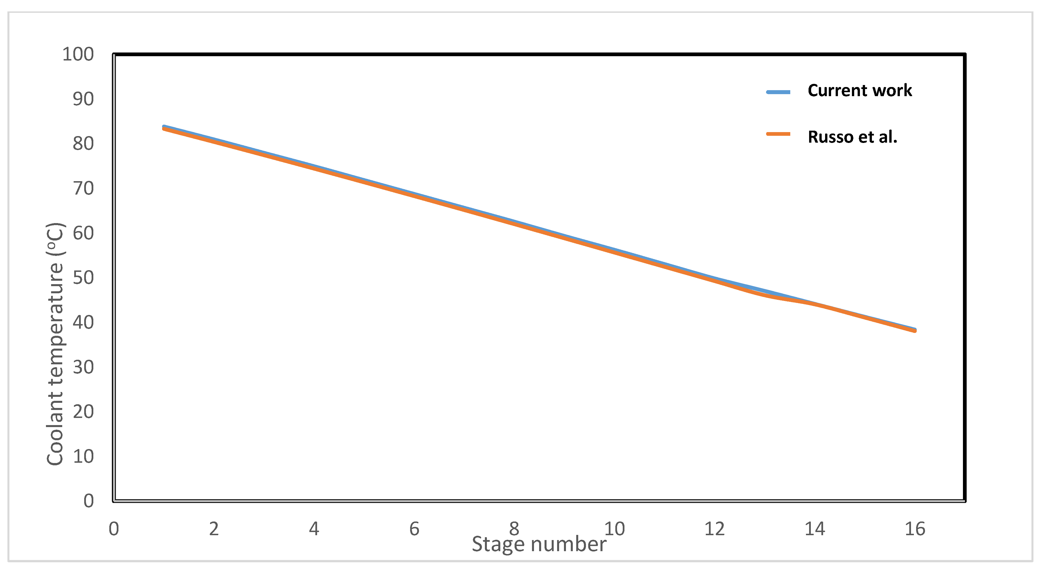
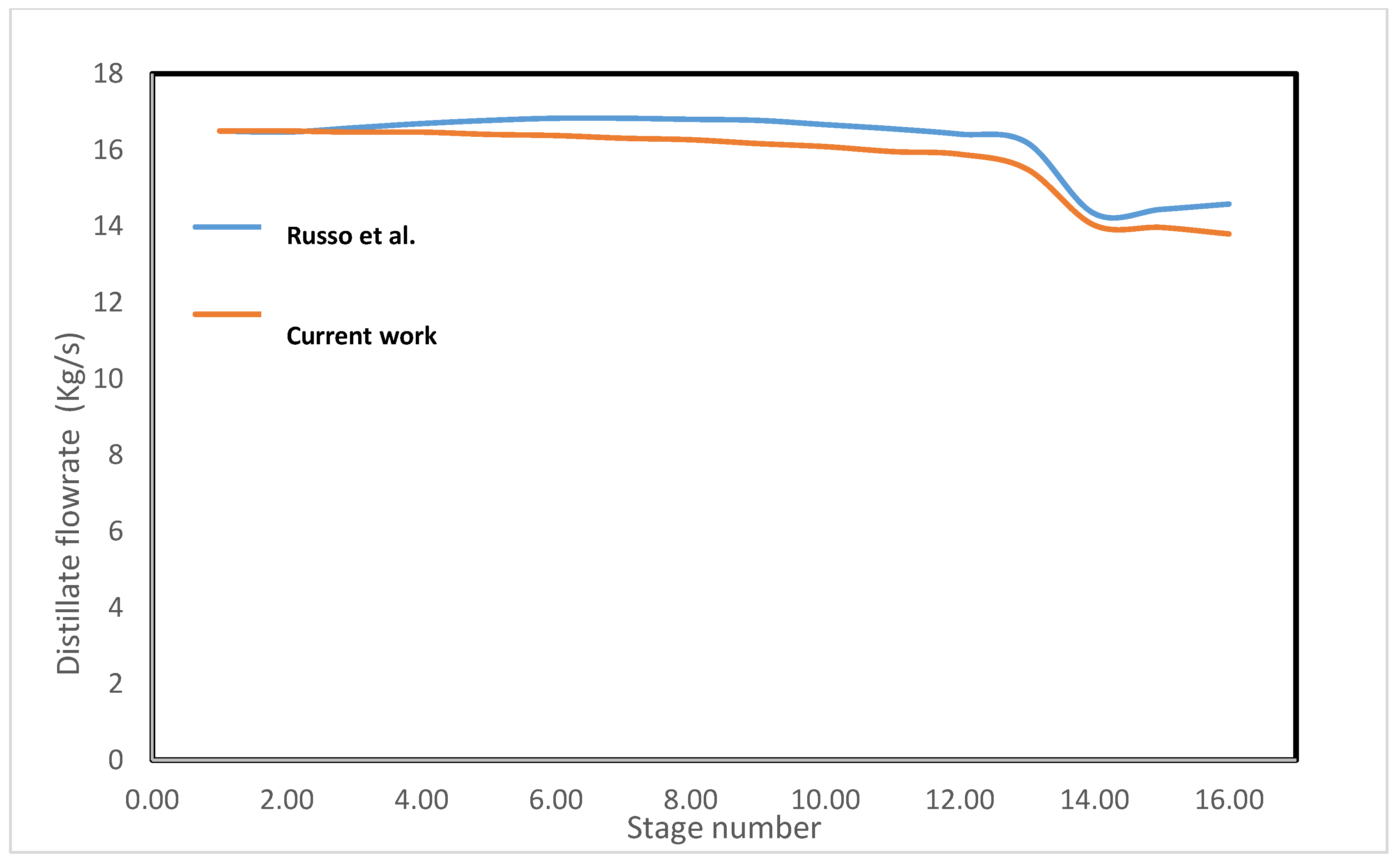
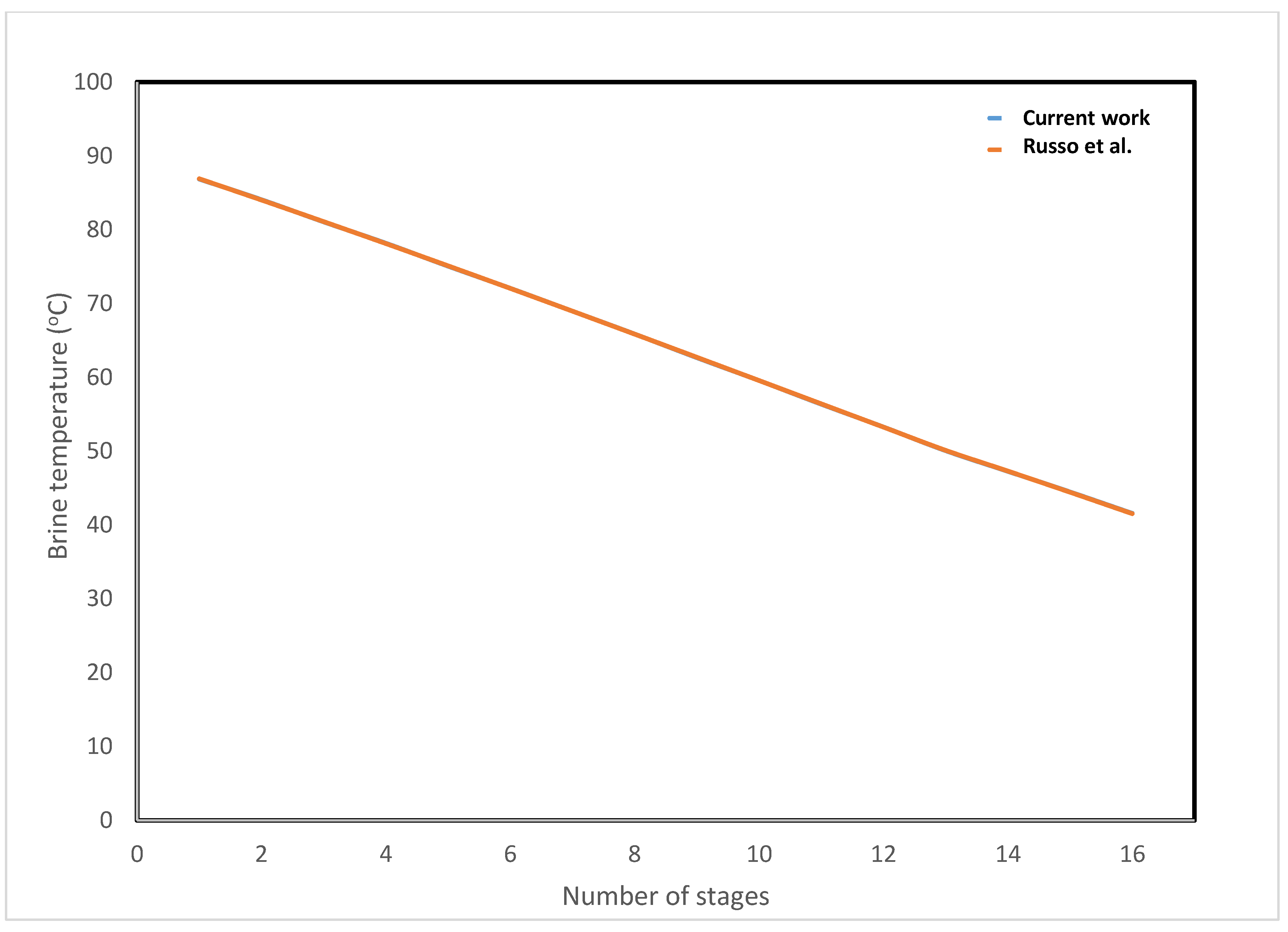
3.1. MSF Model and Validation

In order to calibrate the effectiveness of the hybrid desalination, two MSF desalination designs were initially created with one representing one-through (MSF-OT) while the second represented the brine-recycle model (MSF-BR). Since the current study focuses upon a comparative analysis of the hybrid and MSF processes in terms of scale formation and the overall production of desalinated water, the MSF desalination system created was adequately accurate with respect to the study’s objectives. The configurations of the MSF-OT and BR desalination columns were taken from Russo, et al. [13] and Ali and Kairouani [14] and are shown in Table 1.
The results for brine temperature, coolant temperature and the distillate profiles produced in this study were also compared with those of Russo et al. [13]. These comparisons are shown in Figure 2, Figure 3 and Figure 4.
The brine temperature profiles of Russo, et al. [13] and the current study showed good agreement, with the maximum deviation between these two sets of results being 0.1%.
The maximum deviation in coolant temperature in this study compared to that from Russo, et al. [13] was found to be 2.08%, whereas the maximum deviation in distillate production was 4.5% (<5%). The current study did not consider the contribution of a non-equilibrium allowance in calculating the temperature of the vapour, which might have contributed to the deviations in both the distillate production rate as well as coolant temperature profiles. From these results, it can be concluded that the present model produced in Simulink is in agreement with the modelling data produced by Russo, et al. [13]. In addition, the performance of the current model has been measured in terms of the performance and production ratios. The former was calculated using Equation (62), while the production ratio (PDR) was taken as the ratio between the seawater intake and the distillate output as shown in Equation (58):
P D R =   D t o t M f
For the case of MSF-OT, the performance ratio of the system was calculated to be 9.446, while the production ratio of the system was 0.076. The lower production rates can be attributed to the lack of brine recycling, where the total water wastage in the form of brine would be higher in the MSF-OT model. These values could be further explained by a cross-comparison of MSF-OT with the BR model. Even though there were no heat rejection and heat recovery sections in the MSF-OT model, the heat transfer area of the final three stages, which would have represented the heat rejection section, was maintained at a level equal to the heat transfer area of the heat rejection section in MSF-BR. In the brine recycle model, the flow rate of recycled brine and the seawater intake were chosen in such a way that the initial temperature of the inlet coolant water into the condenser tubes of stage 16 would not be affected (see Figure 1a). The same amount of rejected seawater from the coolant section after the heat rejection section was substituted for the brine in stage 16 (Figure 1b), where the inlet coolant temperature decreased to a lower value, thus increasing the distillate flow rate. Hence, the final performance ratio increased slightly to 9.671, and the total production of brine was 258.1 kg/s against a distillate production from MSF-OT of 252.1 kg/s. However, the production ratio of the system was considerably improved to a value double that of the MSF-OT column (0.1652).

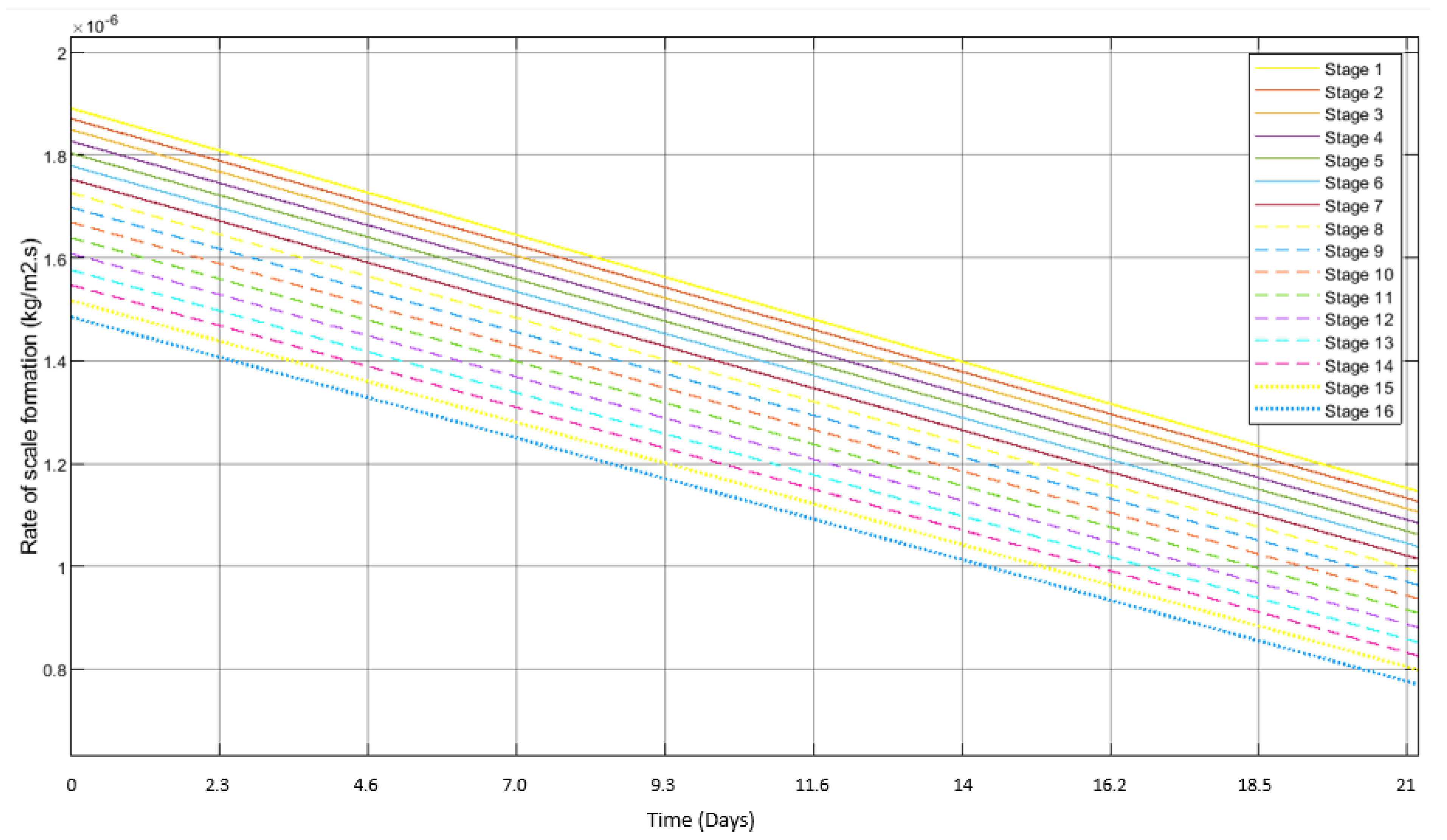
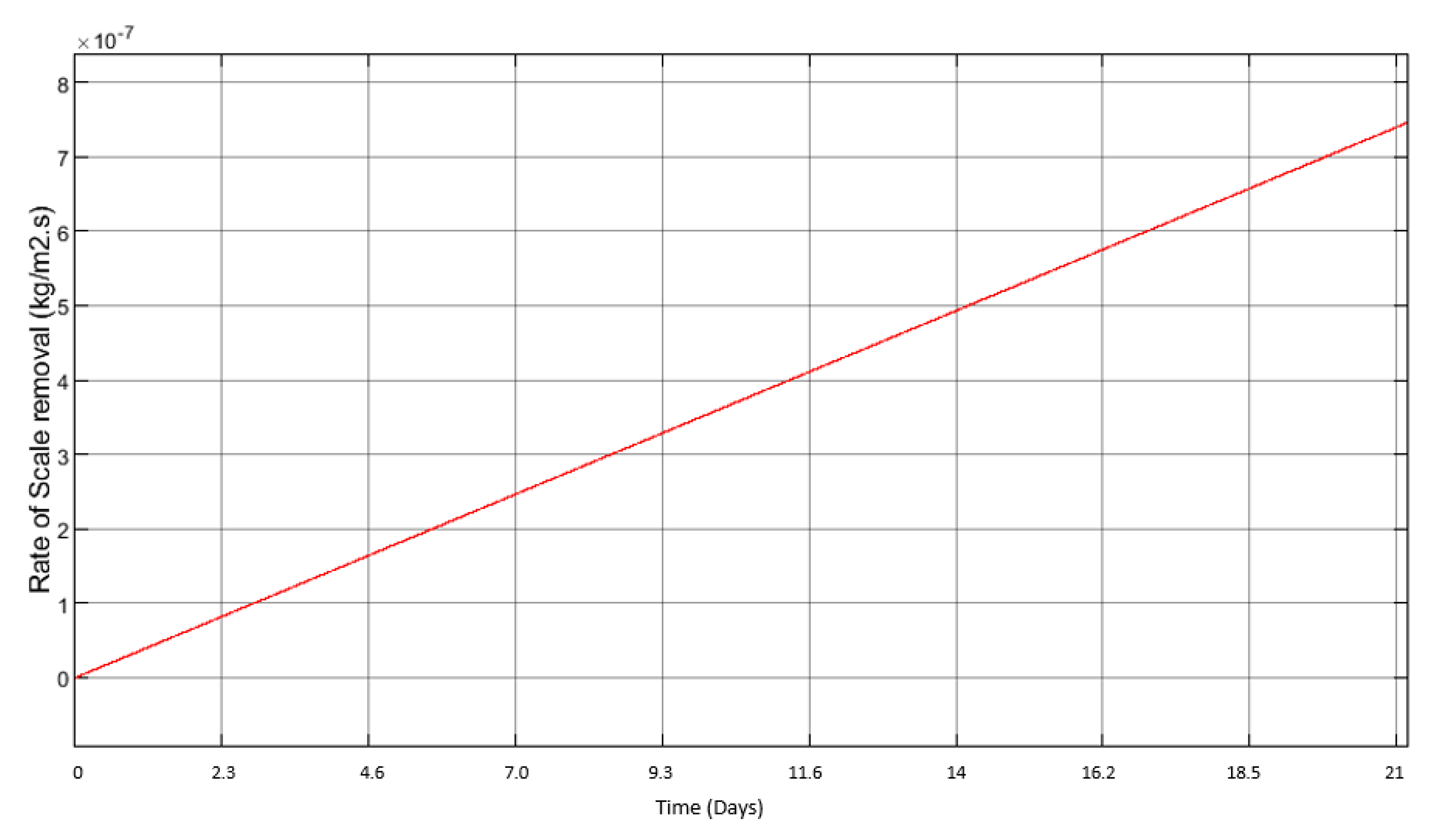
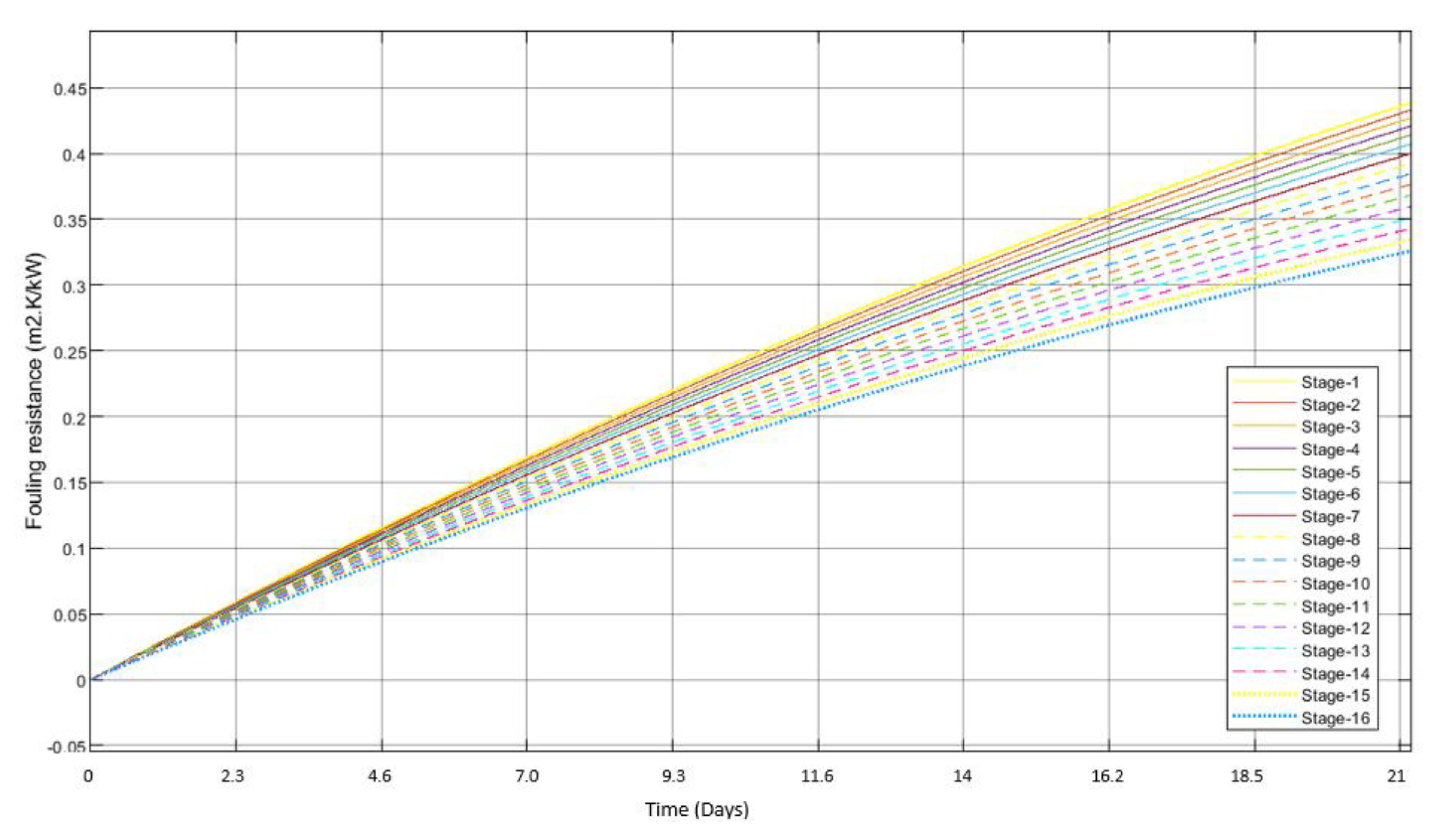
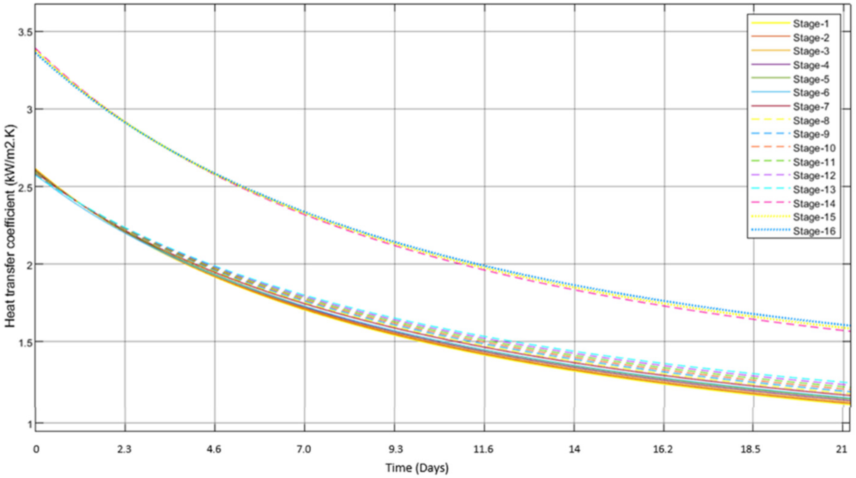
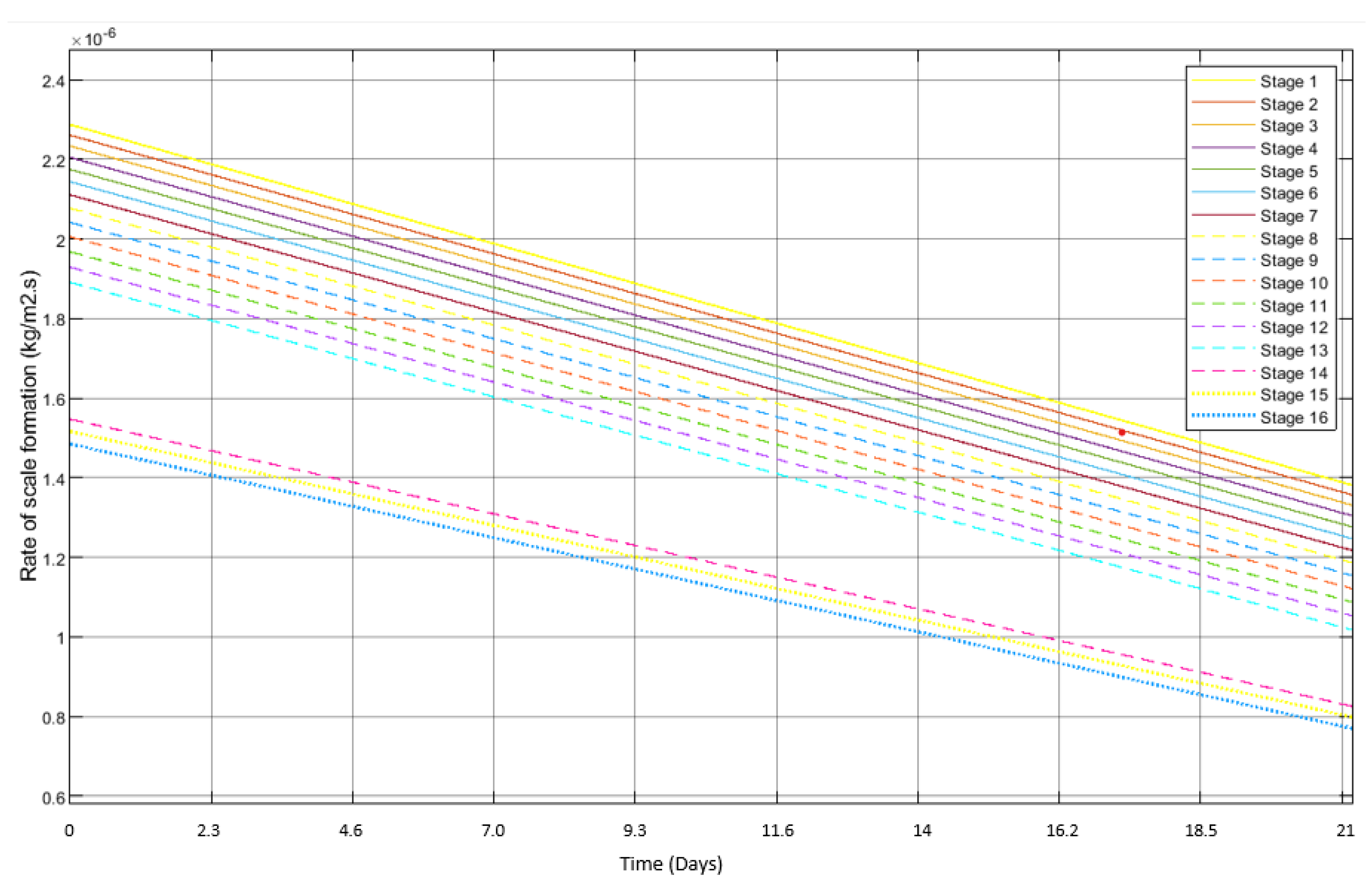
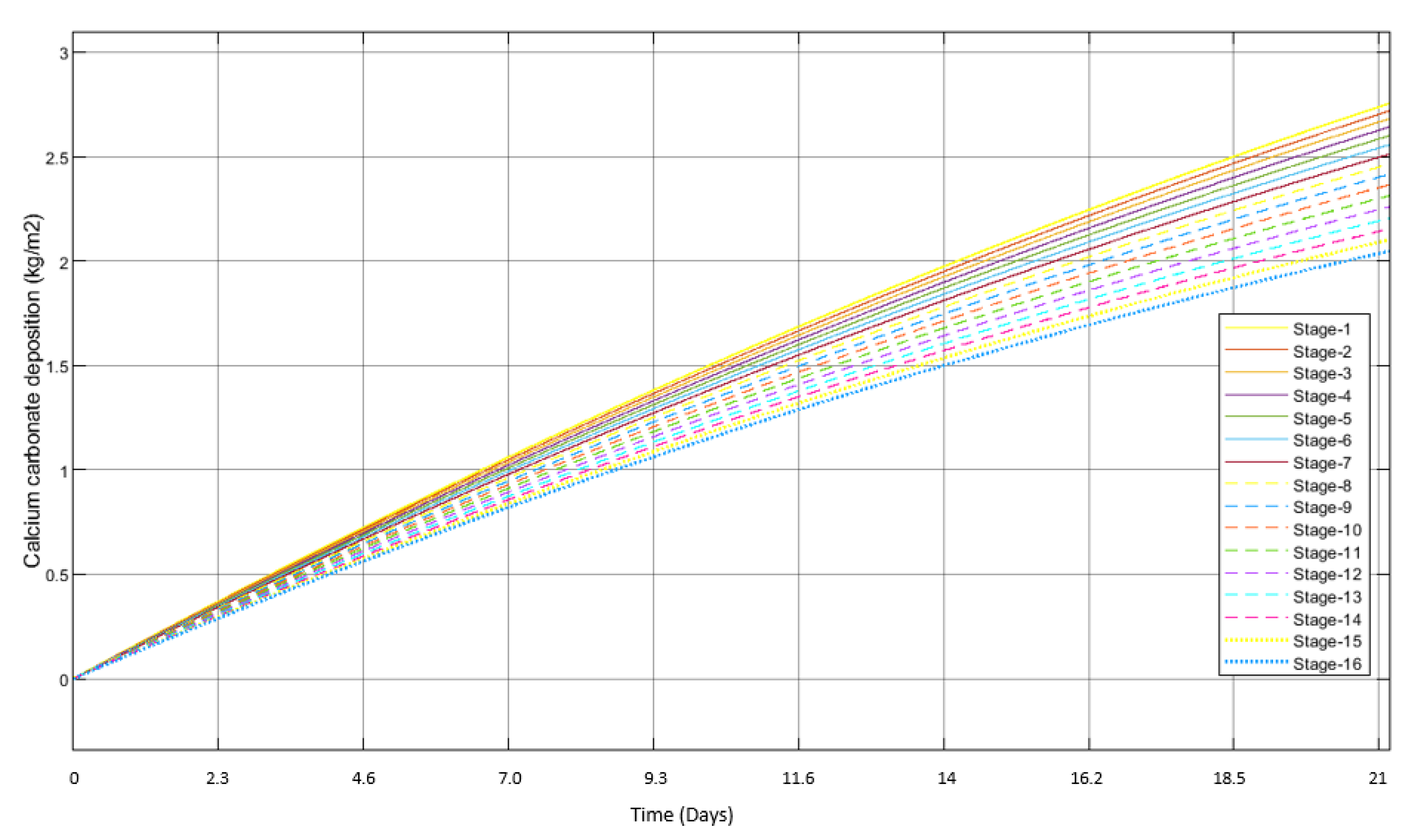
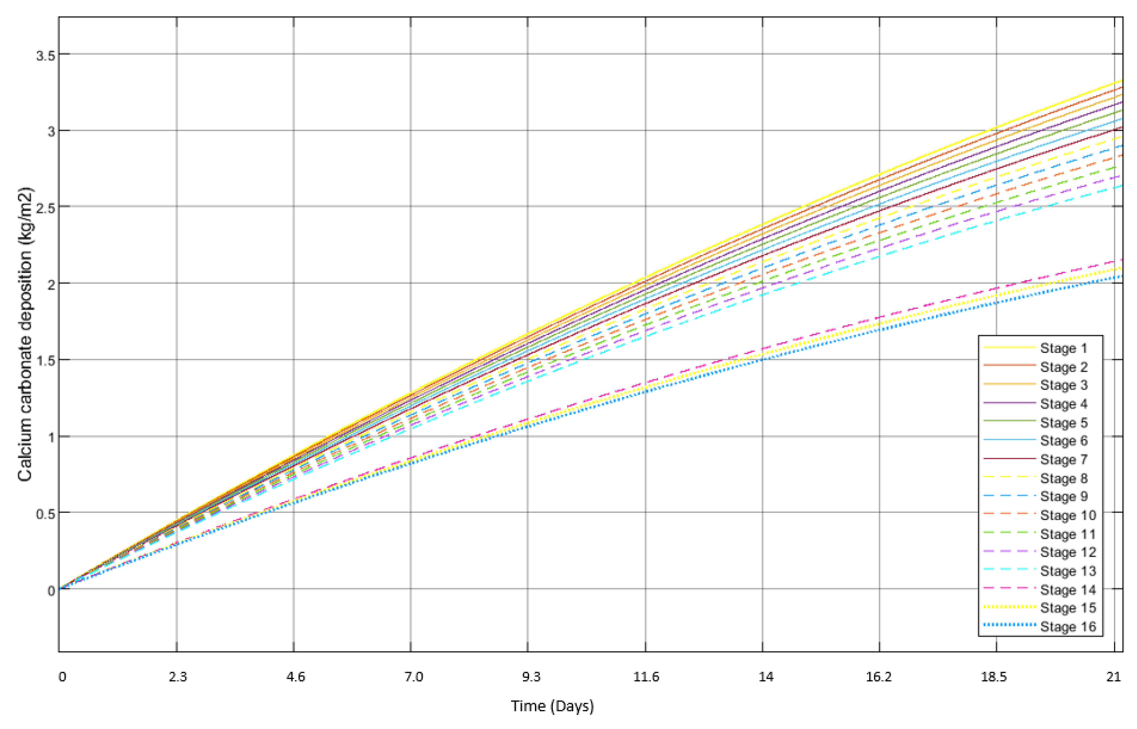
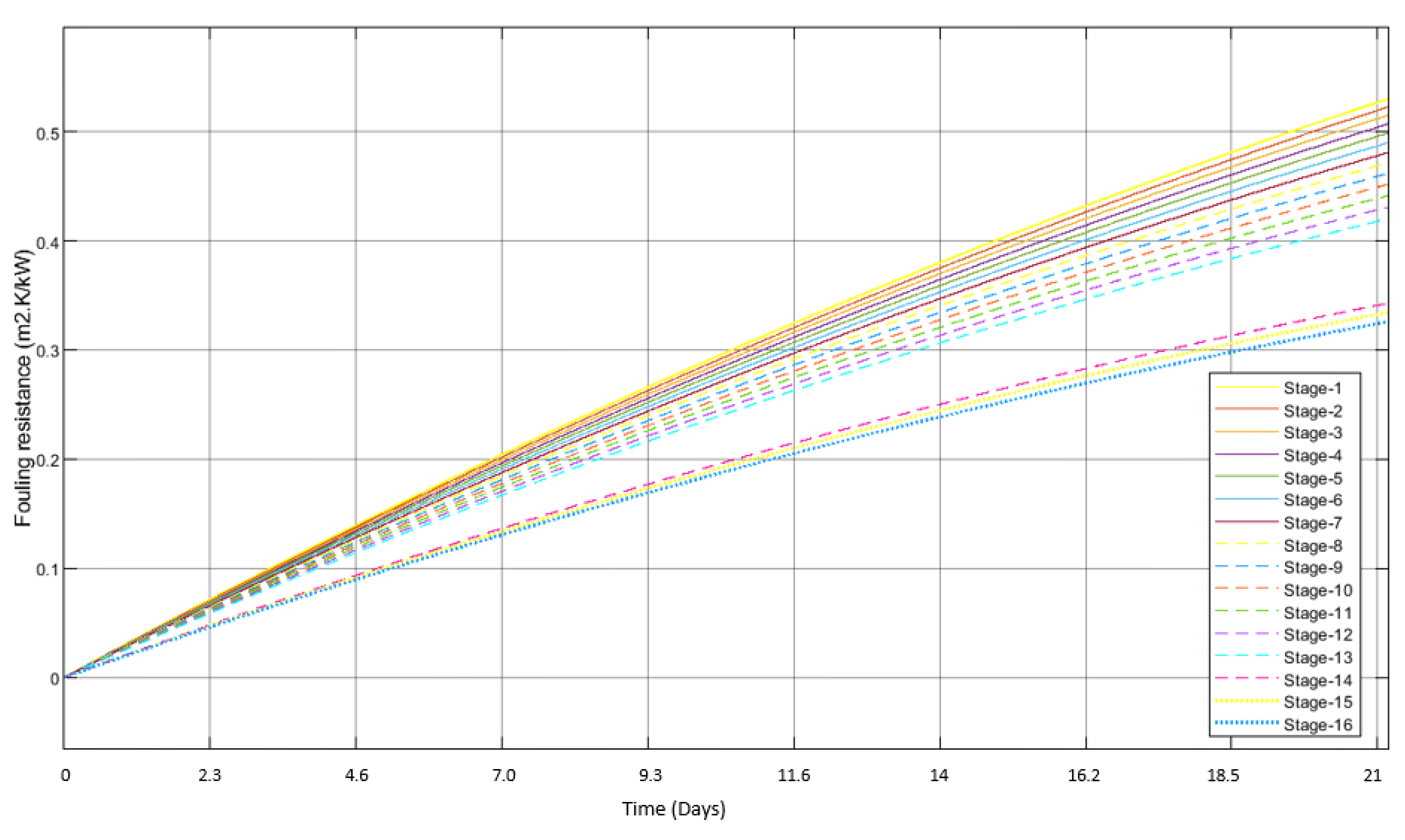
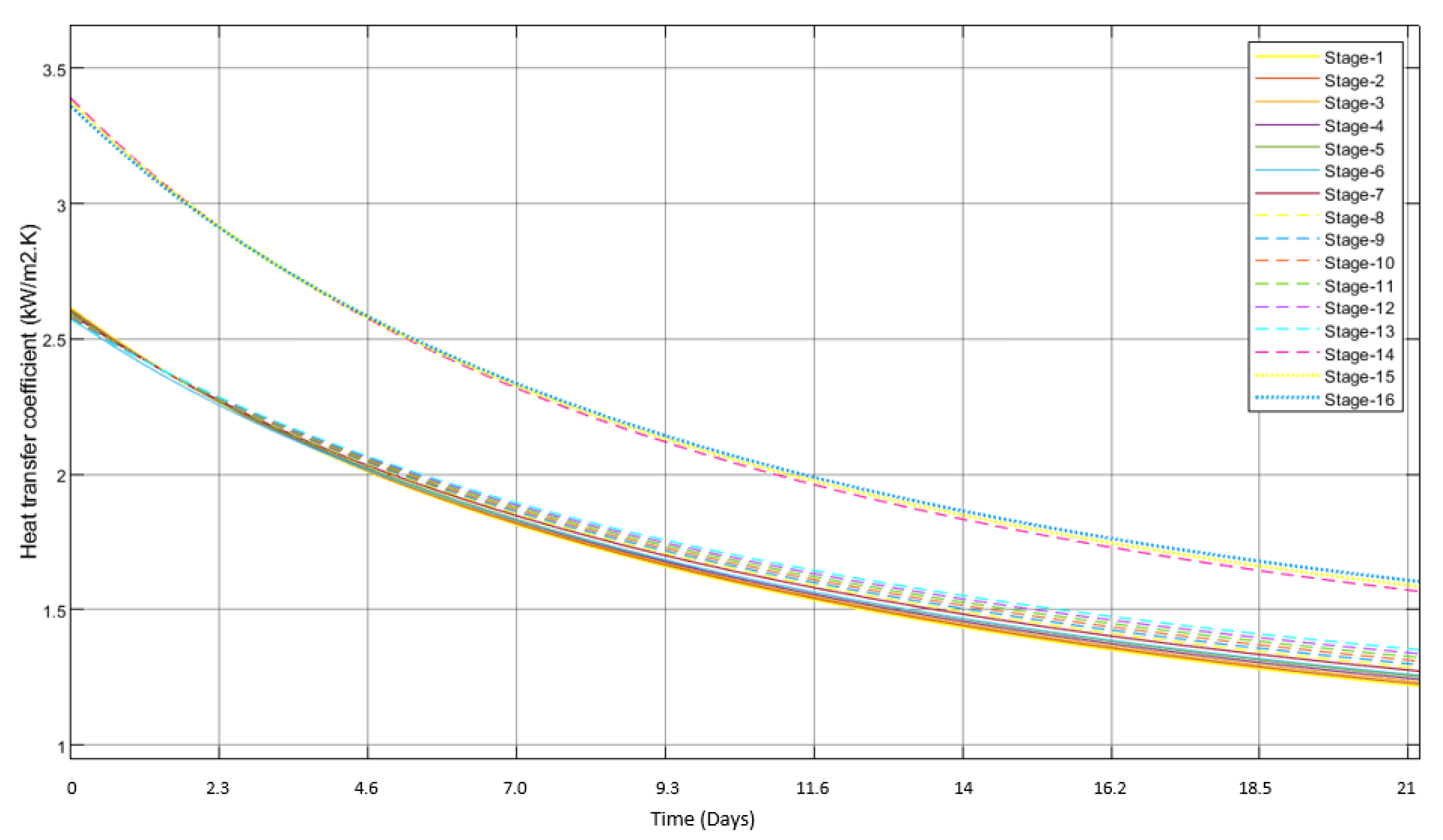
3.2. Scale Formation

The fouling rate profiles will take different shapes under different conditions, and the contributory factors for scale formation are pH, temperature, ion concentration, and pressure. However, in this study, only the parameters of temperature and saline concentration were considered. Scale formation in the first stage has been explained extensively by various authors, while that in the rest of the stages has been mentioned when a comparative analysis is required. For example, Figure 5 shows the overall scale formation in all of the 16 stages of MSF-OT, while Figure 6 shows that for MSF-BR. From these figures, it can be seen that scale formation in MSF-OT and MSF-BR was very different, where the initial scale formation varied from 1.88 × 10⁻⁶ kg/m2·s to1.48 × 10−6 kg/m2·s. In the MSF-BR desalination column for the heat recovery section from stages 1 to 13, the initial scale formation ranged from 2.28 × 10⁻⁶ kg/m2·s to 1.89 × 10⁻⁶ kg/m2, whereas in the heat rejection section in stages 14 to 16, the values varied from 1.55 × 10⁻⁶ kg/m2·s to 1.48 × 10⁻⁶ kg/m2·s.
One of the main concerns with the scale formation plots is their profile shapes. Although many authors have found the profiles of these rates to fit on almost a straight line [7], others have found the profiles to be almost asymptotic [6]. However, it is important to understand that there is no universally accepted observation of the profiles of scale formation since their shapes are highly dependent upon the configuration of the MSF. Evidently, even in the scale formation curves produced by Alsadaie [6], the curvature of the profiles decreased at the lower top brine temperature (TBT) conditions. However, the extent of scale formation was found to be somewhat higher in this study since the elevation of scale removal rates due to the narrowing of the tubes was not taken into consideration. Nonetheless, the scale formation results were still comparable to those of Alsadaie [6].
From the perspective of scale formation, which is highly sensitive to salt concentration, one of the major differences between MSF-OT and MSF-BR is the heightened salt concentrations due to the mixing of brine in the heat recovery section. The effect of salt concentration on scale formation can be clearly seen in Figure 6. In addition, the effect of temperature on scale formation rates is also shown in these figures to decline from the lower stages to the higher stages. It is also seen that the temporal rates of scale formation decreased in all of the stages. This reduction is attributed to the increase in removal rates (and not to the narrowing of the tubes), and the rate of removal in the first stage of the MSF-OT is presented in Figure 7.
The rates of scale formation were used to calculate the extent of aragonite (CaCO3) deposition on the heat transfer surface in the condenser tubes. Similar to the observations in studies by Shams El Din, et al. [5,39], aragonite deposition was found in all of the stages of the MSF in both the OT and BR columns [5,39,40]
In both Figure 8 and Figure 9, the profiles of CaCO3 scale deposition follow the same trend. As with the observations in Figure 6, there is a visible hiatus in the aragonite temporal deposition curves in the MSF-BR desalination column, where a gap can be seen between the heat rejection and heat recovery sections.
As shown in Figure 9, the total aragonite deposition after 21 days (approximately 500 h) was 3.195 kg/m2, which, if equally distributed amongst the 4300 tubes, would give each tube an average deposition of 0.743 g/m2.
Various interpretations of the relationship between flow velocity and fouling resistance have been reported, although a majority of researchers believe that an increase in flow velocity will result in lower fouling resistance [32,33]. It was inferred that the velocities will support the dominance of diffusion over the reaction upon the mass deposition. Generally, these velocities are as low as 0.2 m/s [7], whereas velocities above 1.5 m/s represent the marginal influence of reaction step in governing fouling resistance [23,37].
Hence, the current model considered both diffusion as well as reaction in calculating mass deposition and fouling resistance. Stagewise profiles of thermal resistance by scale formation (fouling resistance) found in various stages of MSF-OT and MSF-BR are shown in Figure 10 and Figure 11. In order to calculate the thermal resistance provided by fouling, information on the density as well as thermal conductivity of the materials was needed. Since the systems were operating under low TBT conditions, considering pure aragonite scale formation, these values were taken from [41,42], respectively. While calculating these values, the fouling layer was assumed to be porous at a value of porosity considered to be 10% with voids filled with water.
From Figure 10 and Figure 11, the shapes of the fouling resistance profiles were found to be similar to those for the mass deposition of aragonite. In case of MSF-OT, the fouling resistance after 21 days resulted in a range of values from 0.35 to 0.44 m2 K/kW, whereas the corresponding values varied from 0.35 to 0.53 m2 K/kW in the case of MSF-BR. The higher fouling resistance in the first stages of MSF-BR compared to MSF-OT were the result of higher salinity in the coolant water flowing in the condensers. However, in the final three stages, values of fouling resistances recorded in the MSF-BR were similar to those for MSF-OT. However, the profiles calculated in this study had values of fouling resistance lower than those in [6]. There are two reasons for this. Firstly, the current study considered only the scale formation from aragonite, and Mg(OH)2 scale formation was ignored due to the low TBT operational conditions of the MSF desalination columns considered; secondly, the low TBT resulted in lower temperatures of the coolant water flowing in the condensers. In addition, design factors, such as coolant flow rate and the number of tubes in the condenser, could contribute to the velocity of the stream in the condenser tubes, which could then contribute to scale deposition and fouling resistance. As reported by Alsadaie (2017) [6], the flow velocity varied between 1.8 and 2.2 m/s, while the flow velocity calculated in the current study varied from 1.6 to 1.7 m/s, which confirms that Alsadaie’s design conditions were comparable to those in the current study. From these observations, it is concluded that the fouling resistances calculated in this are satisfactory.
Using the values of fouling resistance along with the other design and operational parameters of the MSF-OT and MSF-BR columns, the overall heat transfer coefficients were calculated. There have been numerous studies that relate heat transfer to scale formation, and heat transfer rates have been observed to decreased by as much as 80% due to the formation of scale [43,44,45,46,47].
However, experimental studies conducted by Watkinson and Martinez [43] of heat transfer in the presence of CaCO3 scale formation resulted in a reduction in the value of the heat transfer coefficient by over 54%. Their design conditions included the velocity of the fluid at 1.57 m/s, which is comparable to that in the current study. The stagewise heat-transfer coefficient profiles are presented in Figure 12 and Figure 13. From these figures, two sets of heat transfer profiles were found in both MSF-OT and MSF-BR. This was because the design parameters for the desalination columns, such as the inner and outer diameters of the tubes and the numbers of tubes in the first 13 and the later 3 stages, were the same for the purposes of comparison. From Figure 12 and Figure 13, it can also be seen that the overall heat transfer coefficients were lower in the first stages and then increased as the stage number increased. Over time, the heat transfer coefficients declined, whereas by the end of 21 days, they were found to be almost 55% lower than the initial values.
The rates of change in heat transfer coefficients were found to be higher in the initial stages when compared to the later stages, which would be due to the coolant water temperature in the condenser tubes. As with mass deposition and fouling resistance, there is a significant gap in the profiles of heat transfer coefficient shown in Figure 13. At the end of 21 days, the heat transfer coefficient had declined by 60%, which is similar to the observations of Watkinson and Martinez [43].
From these results, the distillate production rates were calculated. The overall distillate production rates under the influence of scale formation, as well as the performance ratios of MSF-OT and MSF-BR, are given in Figure 14 and Figure 15. As seen from Figure 14, the initial and final distillate production rates were higher in the MSF-OT model, while at the end of 21 days, the rates were plunged down to the production values approximately 60% lower than the initial values. These lower distillate production rates were caused by both the higher salinity in the heat recovery section of MSF-BR as well as the higher inlet water temperature in the condenser section.
In the case of MSF-BR, the total reduction in distillate production rate after 21 days was observed to be approximately 63%, whereas in the case of MSF-OT, it was 59%. Meanwhile, the initial PRs of MSF-OT and MSF-BR were 8.4 and 7.6, respectively, while after 21 days, their corresponding values were found to be 3.5 and 2.9, respectively. This reduction in PRs with time can be attributed to the formation of scale, despite the conditions of low TBT.

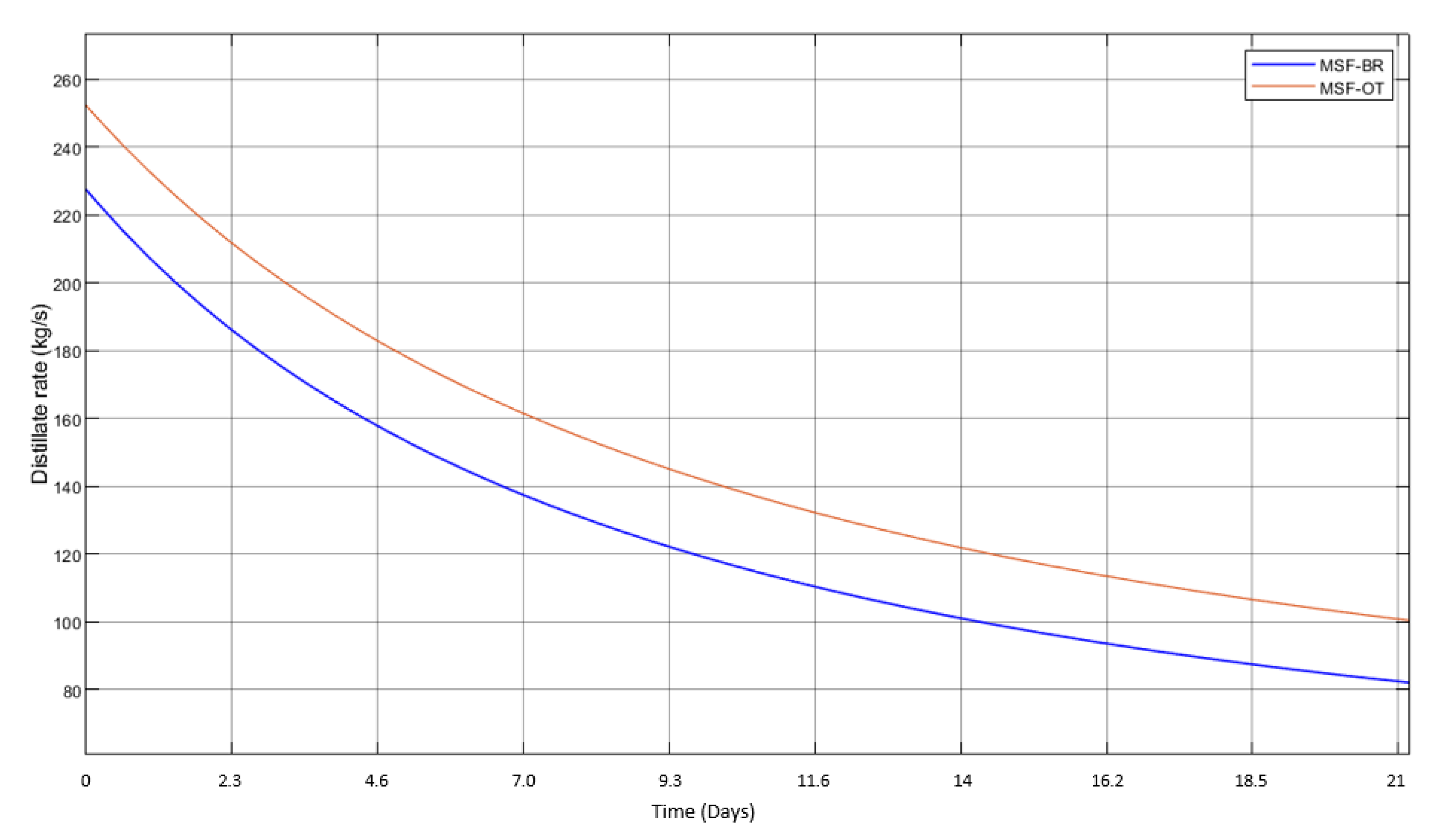
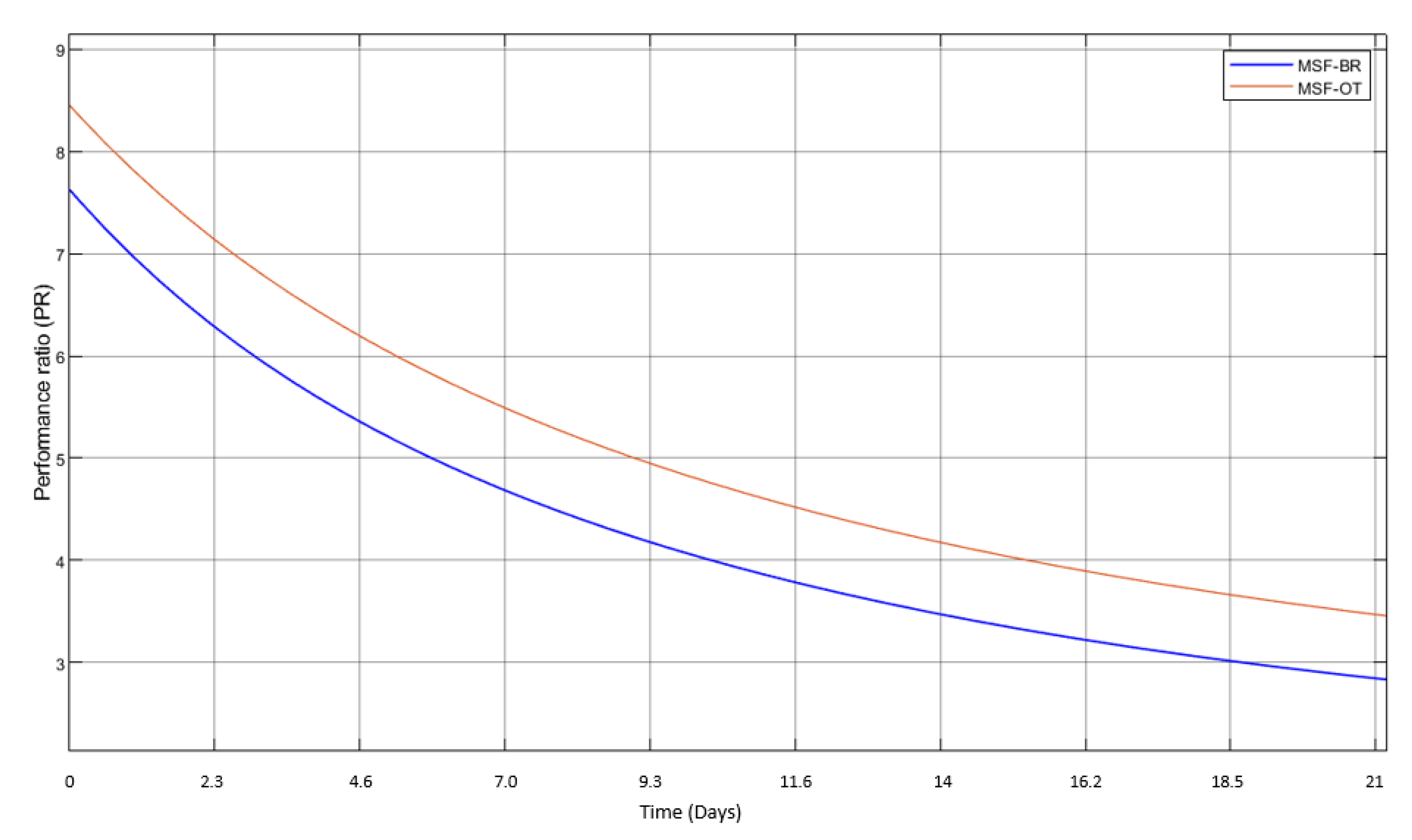
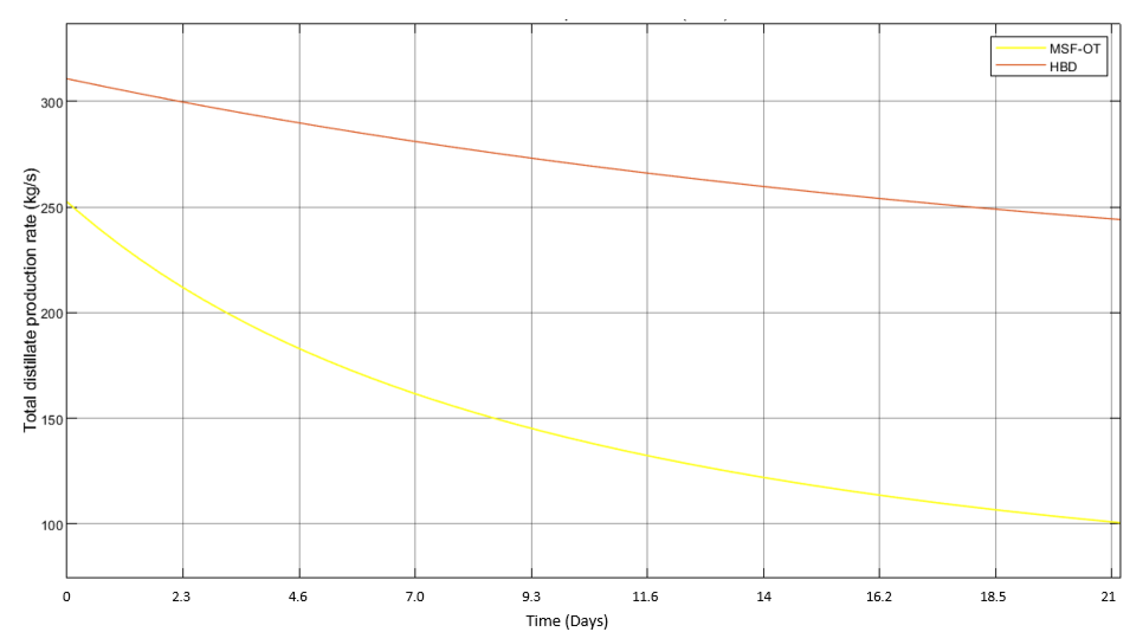
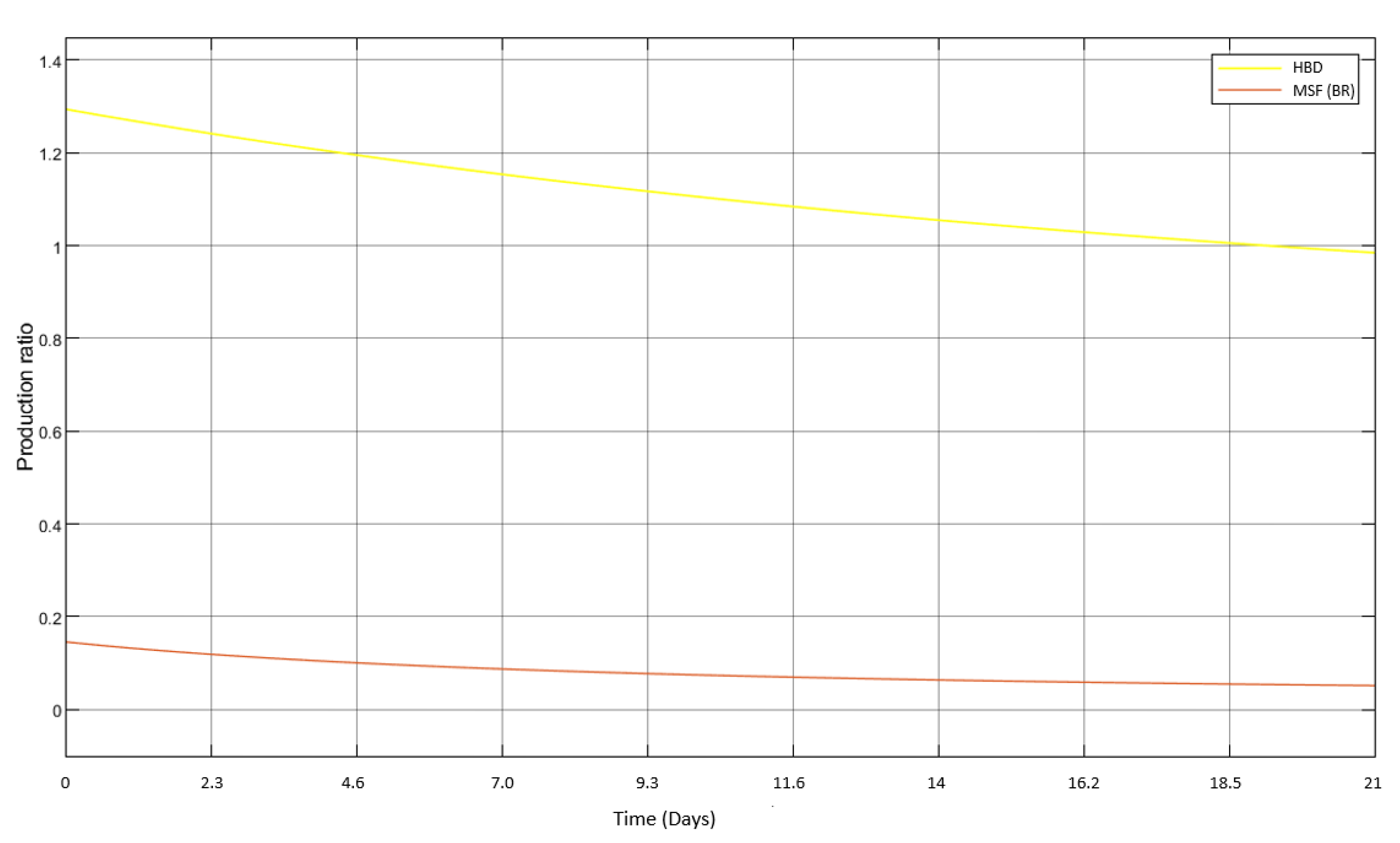
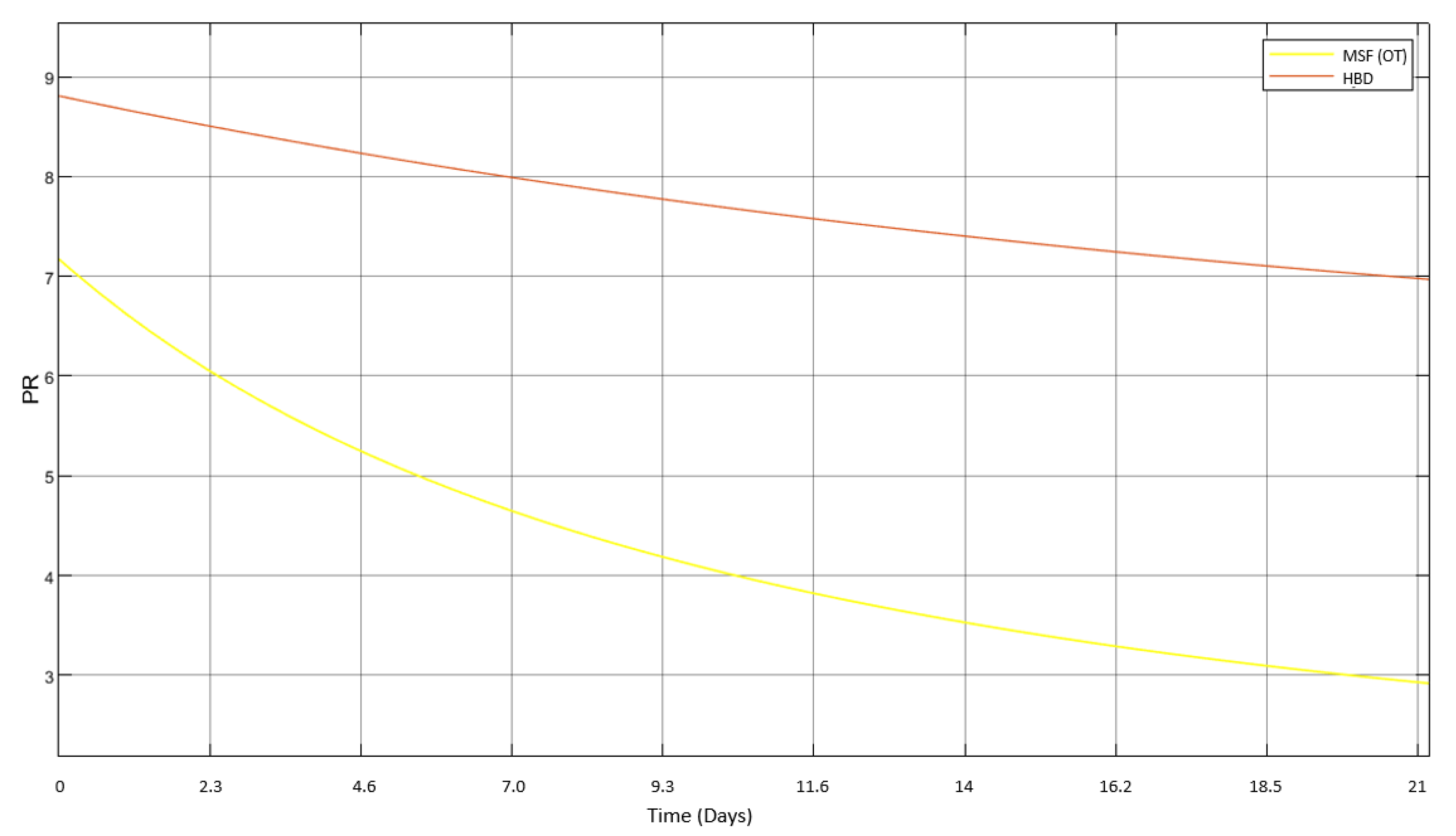
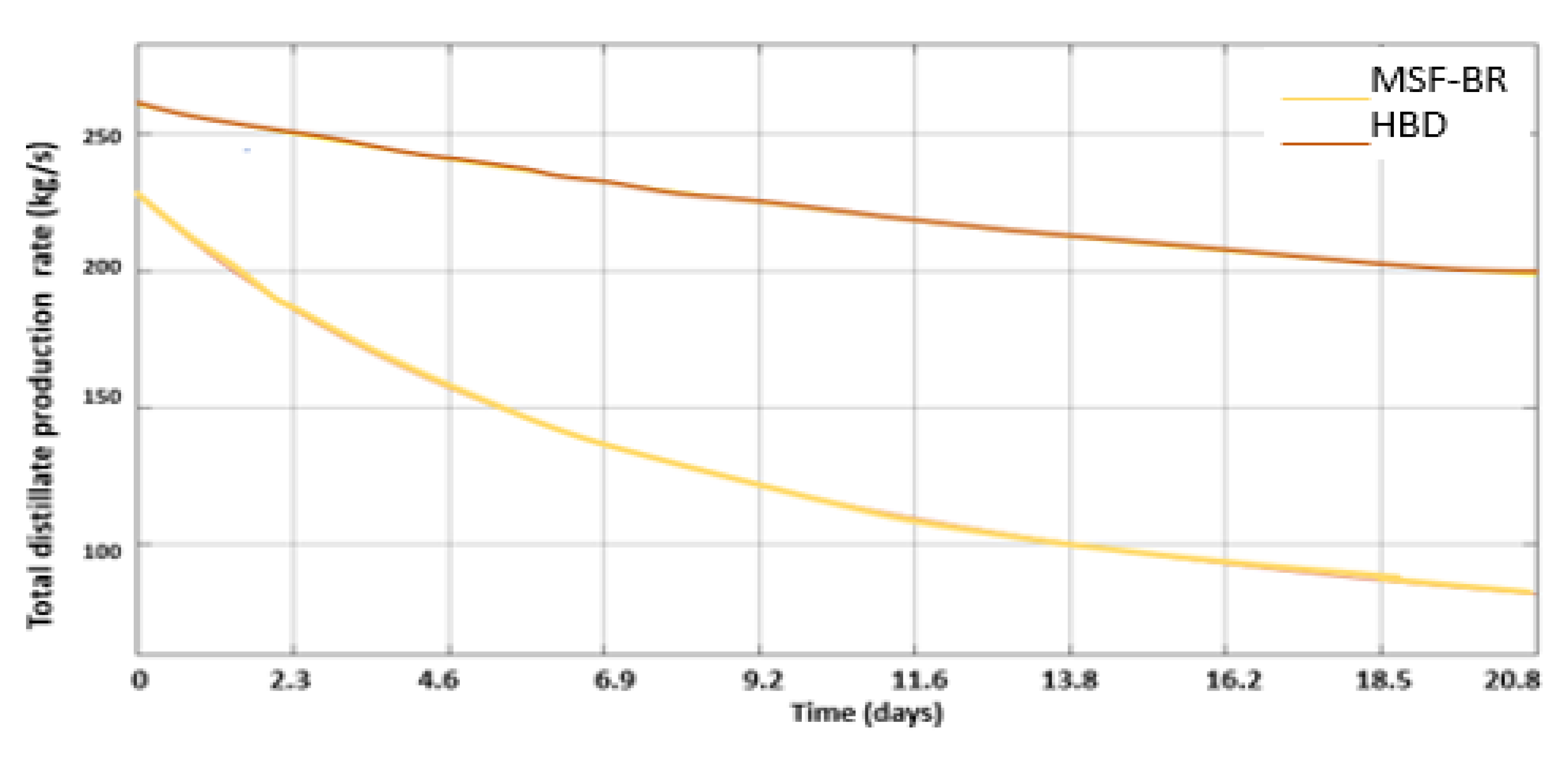
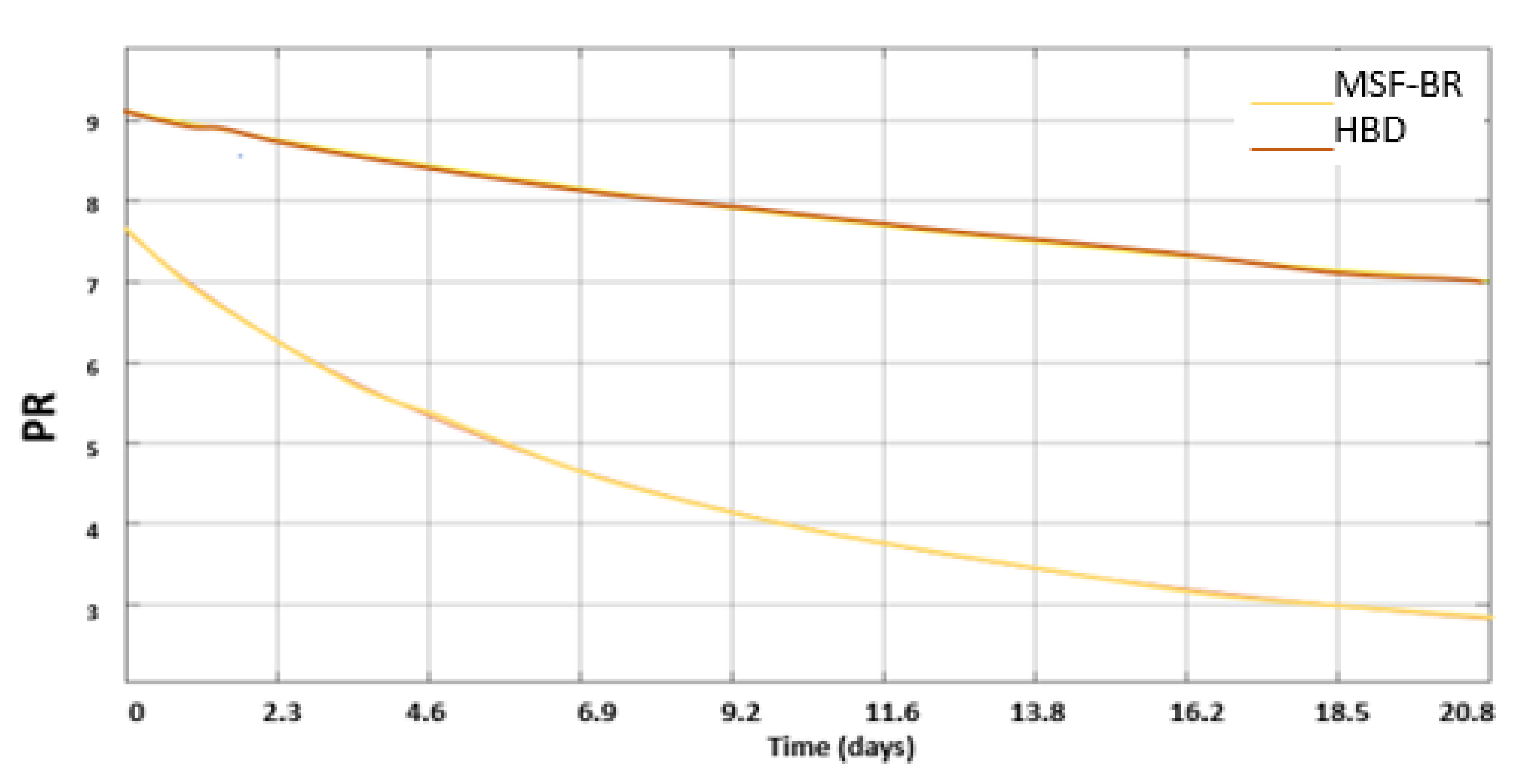
3.3. Introduction of HBD into MSF

In the HBD-MSF system, unlike in conventional MSF distillation columns, the seawater is partially desalinated through the hydrate-based desalination process (HBD; in the current study, CO2 hydrate). The inlet water of MSF after being partially desalinated would consist of lower levels of salts, thus contributing to less scale formation. At the same time, the lower inlet temperatures of the coolant, which would require more coolant recycling (MR), change the production ratio. The hydrate formation experiments conducted in previous studies [15,48,49] give an overall idea of the hydrate formation conditions and the inlet temperatures of water from hydrate counterparts into the MSF coolant section. The rate of hydrate will result into the overall flowrate of hydrate slurry into the MSF coolant section. As the CO2 hydrate is highly sensitive to temperature and pressure conditions, its dissociation would be more likely during the transport of hydrate from the hydrate reactor to the MSF column. In addition, the CO2 hydrates that formed at above 3.5 MPa and 274 K temperatures were observed to be unstable at ambient conditions, causing faster dissociation [50]. To analyse the performance of the hybrid HBD-MSF system, the following configuration was assumed for the hydrate formation process:
(a)
The hydrate would form in the unstirred vessel, where the temporal collection of hydrate would occur. Therefore, HBD acts as a ’precursor’ thsat could, in turn, serve as the process of heat removal for MSF.
(b)
The liquid phase would consist of seawater along with 100 ppm of sodium dodecyl sulphate (SDS), which would be removed along with the brine remnant in HBD.
(c)
The hydrate forming guest gas would be a mixture of 95% CO2 and 5% CH4, where CH4 is considered to be the less hydrate-forming gaseous impurity.
The hydrate formation kinetics, yield, and the extrapolated profiles of water-to-hydrate conversion when the thermodynamic barrier is eliminated, were studied by Thoutam et al., [15] and Thoutam et al., [51]. The performance ratios of the hybrid systems were initially evaluated and then compared with those of their respective MSF-only counterparts.
The profiles of temporal distillate production rates for 21 days of operation are given in Figure 16. As shown in this figure, the overall distillate production of HBD-MSF-OT is higher than the total distillate water production from MSF-OT due to the lower inlet water temperature of the hybrid system. For the MSF-OT system, the inlet water temperature was 311.55 K [14,52], while for the HBD-MSF-OT system, it was 274.15 K [15,50]. Due to these lower temperature conditions of the inlet water, the resulting initial distillate production rate was found to be 311 kg/s, while the corresponding value was 252 kg/s in the case of MSF-OT. After 21 days, this value fell to 100 kg/s for MSF-OT, whereas for HBD-MSF-OT it was 246 kg/s, which was 2.46 times higher than the MSF-OT value.
Similarly, as shown in Figure 17, HBD-MSF-OT showed a considerably better performance than MSF-OT at the initial stages and after 21 days. The initial PR for the HBD-MSF-OT system was calculated to be 8.8, while for MSF-OT, the PR was 7.2. This means that the effect of inlet water temperature from the dissociated hydrate improved the initial performance ratio by a factor of 1.22. Due to scale formation, the performance ratio after 21 days was found to have fallen to a value of 2.96 for the MSF-OT system. The previous experimental studies of HBD-MSF-OT showed a salt removal level of 74.5% [15]; hence, the salinity of the inlet water in the case of the HBD-MSF-OT system was 8.925 mg/g against a value of 35 mg/g in the inlet stream of MSF-OT. It is worth mentioning that, despite the salinity difference of inlet water stream, the amount of water into MSF with and without HBD was kept constant at 3340 Kg/s to indicate the dependency of the PR and the distillate water production of MSF to water salinity and temperature. The changes in temperature for each stage are presented in Figure 2 and Figure 3, which were used for performance evaluation of MSF with and without HBD.
Thanks to the lower salinity values obtained by the HBD process, the final PR of the MSF counterpart of the HBD-MSF-OT system was calculated to be 7.025. This value is 2.37 times higher than the final PR of the MSF-OT system.
An approach similar to the integration of HBD into MSF-OT was performed for the integration of HBD into MS-BR. However, the operation of HBD in MSF-BR differed from that of MSF-OT. In the latter, the entire coolant water inlet of the HBD-MSF-OT was provided by the dissociated hydrate, while in the case of HBD-MSF-BR, the ratio of brine recycle and dissociated hydrate intake was maintained in such a way that the inlet coolant temperature was maintained at a temperature of 317.25 K [13]. This temperature was calculated considering the ratio of brine recycle to the total brine flow rate in the condensers (the recycle ratio), as given in [13], along with the consideration of a seawater temperature of 311.55 K as in the case of MSF-OT. The initial brine recycle ratio was 0.503, whereas the brine recycle ratio in HBD-MSF-BR was calculated to be 0.936. This means that the requirement of excess water input from outside of the MSF was 7.75 times lower in the case of HBD-MSF-BR compared to MSF-BR.
The overall distillate production rates for HBD-MSF-BR in comparison to MSF-BR, as shown in Figure 18, were initially considerably higher, at 1.14 times the production rates of MSF-BR. This was due to the low salinity of the inlet water. At the end of 21 days, the production rate of distillate had fallen to 84.07 kg/s in the case of MSF-BR. This was a reduction of approximately 63% compared to the initial rate. However, due to the lower salinity contributing to less scale formation and the higher heat transfer rates in the condensers, the final production rates were calculated to be 200.3 kg/s. This is equivalent to a reduction in the initial value of approximately 23%.
A similar trend was observed in case of the performance ratio when compared the PR of HBD-MSF-BR with MSF-BR models, the profiles of which were shown in the Figure 19.
In the case of MSF-BR, the initial PR was observed to be 7.75, whereas in the HBD-MSF-BR, this value was 1.17 times higher at 9.10. The initial value of PR was mainly affected by the requirement of more steam due to the higher outlet temperature of the coolant stream from stage 1 of MSF-BR. Due to the higher salinity of the inlet water, which was further increased by the recycled brine from the last stage of the flash chamber, the PR of the MSF-BR fell by 62.6% after 21 days of operation. However, this plunge was calculated to be only 22% in the case of the hybrid system. The HBD-MSF-BR system recorded a final PR of 7.08, which was 2.44 times higher than that of MSF-BR.
Alongside the performance ratio, the production ratio (PDR) was also calculated for desalination systems in order to analyse the water wastage. The PDR is the ratio of the distillate produced from the MSF desalination column to the inlet seawater from outside of the MSF desalination column. As there was no brine recycling in the MSF-OT and HBD-MSF-OT systems, the entire amount of water flowing in the condensers serves as the denominator for the production ratio, which will hence be a relatively smaller quantity compared to BR models.
Even though the denominator was same for both the HBD-MSF-OT and MSF-OT systems, the production ratios of these systems turned out to be different from each other due to the variable rates of distillate production. As seen in Figure 20, total distillate production rates were higher in the HBD-MSF-OT system when compared to the MSF-OT system, which led to the higher production rates of HBD-MSF-OT in both the initial and final phases of the period of 21 days. With a similar approach, Figure 21 shows the profiles of the temporal production ratios of the MSF-BR and HBD-MSF-BR systems. As seen from this figure, the production ratio of the BR system was considerably higher than that of the OT system due to the brine recycling. From Figure 21, much higher production ratios were seen in the case of HBD-MSF-BR when compared to MSF-BR. This was due to the higher rates of brine recycling needed to attain the same inlet temperature of water into the condenser tubes for the energy rejection system of the MSF-BR counterpart.
From the perspective of desalination, the HBD based pre-treatment would improve the overall performance of MSF by reducing scale formation, and the lower temperature of dissociated hydrate would reduce the freshwater intake needed to maintain the same amount of distillate. Based on the current work, the scale formation rates were 40.6% and 36.3% lower for the hybrid HBD-MSF-OT and HBD-MSF-BR systems, respectively.

4. Conclusions

The performance ratios (PRs) and production ratios (PDRs) of the MSF-BR and MSF-OT systems considered were calculated over time and compared to the values for the hybrid HBD-MSF-OT and HBD-MSF-BR systems. The results show that the pre-treatment of seawater by HBD had a considerable beneficial influence in improving the performance of the MSF system. The simulation results show that the integration of HBD into MSF-BR enhanced the PR by 17%, while a value of 22% was recorded for the MSF-OT system.
The rate of decline of the PR for MSF-OT was calculated to be 62.6% after 21 days of operation. However, this value for HBD-MSF-BR was only 22%. The same trend for the reduction in the PR was observed for MSF-BR and HBD-MSF-BR, with the corresponding reductions in PR for MSF-BR calculated to be 58.8% and 22.5%, respectively. The enhancement of PR for hybrid systems can be attributed to the lower temperature and salinity of the outflux from the hybrid system as well as the higher brine recycling ratio.
Due to the higher quality of the output water from the hybrid system in terms of salinity and temperature, the pre-treatment process through the hybrid process improved the performance of MSF by lowering scale formation rates considerably in the hybrid HBD-MSF-OT and HBD-MSF-BR systems, where the scale formation rates fell by 40.6% and 36.3%, respectively.

Author Contributions

Conceptualisation, P.T. and S.R.G.; methodology, P.T. and S.R.G.; software, P.T.; validation, P.T., S.R.G. and F.A.; formal analysis, P.T.; investigation, P.T. and P.A.S.; resources, P.T., P.A.S., F.A., H.A., I.A., A.A.-s., E.A., O.B. and S.R.G.; writing—original draft preparation, P.T. and P.A.S.; writing—review and editing, S.R.G., F.A., H.A., I.A., A.A.-s., E.A. and O.B.; supervision, S.R.G. and F.A.; project administration, S.R.G., I.A. and H.A. All authors have read and agreed to the published version of the manuscript.

Funding

The authors would like to thank the Deputyship for Research and Innovation, Ministry of Education in Saudi Arabia, through project number IFPNC-002-135-2020 and King Abdul-Aziz University DSR, Jeddah, Saudi Arabia for funding this research.

Data Availability Statement

Data sharing is not applicable to this article as no new data were created in this study.

Acknowledgments

The authors would like to express their appreciation to Teesside University for providing the facilities and software to perform the modelling.

Conflicts of Interest

The authors declare no conflict of interest.

Abbreviations

βMass transfer coefficient reaction, m/s
µBrine viscosity, kg/m s
µRRelative viscosity
µwbrine viscosity at wall, kg/m s
AHeat transfer area, m2
aa, baDebye–Huckel parameters specific to ion ‘a’
AcrossTube cross-section area, m2
ADH, BDHDebye–Huckel constants
BBrine flowrate, kg/s
BDHTemperature dependent Debye–Huckel constant
CbIon concentration in the bulk stream, kg/m3
CiIon concentration at the liquid–solid boundary layer, kg/m3
CpSpecific heat at constant pressure, kJ/kg °C
CsSaturation concentration, kg/m3
DDiffusion coefficient, m2/s
DhHydraulic diameter of the tube, m
DiDistillate flowrate, kg/s
diInner diameter of the condenser tube, m
doOuter diameter of the condenser tube, m
EaActivation energy, kJ
fFanning friction factor
gGravitational acceleration, m/s2)
hinInside heat transfer coefficient, W/m2·K
houtOutside heat transfer coefficient, W/m2·K
kDCoefficient of mass transfer, m4/s·kg
krReaction rate constant, m4/s·kg
kremRemoval rate constant, m3/s·kg
KspSolubility product, mol2/kg2
ktubeThermal conductivity of the tube, kW/m·K
LMTDLog mean temperature difference, °C
MCRRecirculated coolant mass flowrate, kg/s
McwMass flow rate of colling water, kg/s
mdProgressive deposition rate, kg/s·m2
MfIntake seawater, kg/s
mfNet scale deposition, kg/s·m2
miMolality of the dissolved gas, mol/kg
MRFlow rates of recycled brine, kg/s
mrMass removal rate, kg/s·m2
NNumber of defects in the fouling layer
POperational pressure, MPa
ReReynolds number, Equation (43)
RfThermal resistance, °C/kJ
rfiHeat transfer resistance on the inside of the condenser tube, m2·°C/kW
rfoHeat transfer resistance on the outside of the condenser tube, m2·°C/kW
ScSchmidt number
TbBrine temperature
TdiTemperature of vapour after passing through the demisters, K
TfTemperature of the coolant, K
TsSurface temperature inside the tubes, K
TvTemperature of vapour, K
UOverall heat transfer coefficient, kW/m2·°C
UcOverall heat transfer coefficient, kW/m2 °C
vFriction velocity, m/s
VelVelocity of the coolant stream flowing inside the condenser tubes, m/s
XSalt concentration, g/kg
xi Mole fraction of dissolved gas in liquid
xfLayer thickness, m
ZCompressibility factor
ZiCharge number of ion ‘i’
ZaIonic charge on the ion ‘a’
λfThermal conductivity, kJ/m °C
λvThe latent heat of vapour, kJ/kg
λcLatent heat of condensation
ɣiActivity coefficient
ρfDensity, kg/m3
σfShear strength of the fouling layer, N/m2
δLinear expansion coefficient, °C−1
ΤfSurface shear stress, N/m2
υwViscosity of water, kg/m·s
ρwDensity of water, kg/m3

References

  1. El-Ghonemy, A. Performance test of a sea water multi-stage flash distillation plant: Case study. Alex. Eng. J. 2018, 57, 2401–2413. [Google Scholar] [CrossRef]
  2. Al-Sofi, M.A.K. Fouling phenomena in multi stage flash (MSF) distillers. Desalination 1999, 126, 61–76. [Google Scholar] [CrossRef]
  3. El Din AM, S.; Mohammed, R.A. The problem of alkaline scale formation from a study on Arabian Gulf water. Desalination 1989, 71, 313–324. [Google Scholar] [CrossRef]
  4. Shams El Din, A.; Mohammed, R. Contribution to the problem of vapour-side corrosion of copper-nickel tubes in MSF distillers. Desalination 1998, 115, 135–144. [Google Scholar] [CrossRef]
  5. Shams El Din, A.; El-Dahshan, M.; Mohammed, R. Scale formation in flash chambers of high-temperature MSF distillers. Desalination 2005, 177, 241–258. [Google Scholar] [CrossRef]
  6. Alsadaie, S.M. Design and operation of multistage flash (MSF) desalination: Advanced control strategies and impact of fouling. Ph.D. Thesis, University of Bradford, Bradford, UK, 2017. [Google Scholar]
  7. Hamed, O.A.; Al-Otaibi, H.A. Prospects of operation of MSF desalination plants at high TBT and low antiscalant dosing rate. Desalination 2010, 256, 181–189. [Google Scholar] [CrossRef]
  8. Steinhagen, R.; Müller-Steinhagen, H.; Maani, K. Problems and costs due to heat exchanger fouling in New Zealand industries. Heat Transf. Eng. 1993, 14, 19–30. [Google Scholar] [CrossRef]
  9. Al-Ahmad, M.; Aleem, F.A. Scale formation and fouling problems and their predicted reflection on the performance of desalination plants in Saudi Arabia. Desalination 1994, 96, 409–419. [Google Scholar] [CrossRef]
  10. Song, L.; Lobo, J.D.; Brons, G.B.; Chhotray, S.; Joshi, H.M.; Lutz, G.A. Mitigation of in-tube fouling in heat exchangers using controlled mechanical vibration. ExxonMobil Research and Engineering Co. U.S. Patent Number US7836941B2, 23 November 2010. [Google Scholar]
  11. Pogiatzis, T.; Ishiyama, E.M.; Paterson, W.R.; Vassiliadis, V.S.; Wilson, D.I. Identifying optimal cleaning cycles for heat exchangers subject to fouling and ageing. Appl. Energy 2012, 89, 60–66. [Google Scholar] [CrossRef]
  12. Müller-Steinhagen, H.; Malayeri, M.; Watkinson, A. Heat exchanger fouling: Mitigation and cleaning strategies. Heat Transf. Eng. 2011, 32, 189–196. [Google Scholar] [CrossRef]
  13. Rosso, M.; Beltramini, A.; Mazzotti, M.; Morbidelli, M. Modelling multistage flash desalination plants. Desalination 1997, 108, 365–374. [Google Scholar] [CrossRef]
  14. Ali, M.; Kairouani, L. Solving equations describing the steady-state model of MSF desalination process using Solver Optimization Tool of MATLAB software. Desalination Water Treat. 2014, 52, 7473–7483. [Google Scholar] [CrossRef]
  15. Thoutam, P.; Rezaei Gomari, S.; Chapoy, A.; Ahmad, F.; Islam, M. Study on CO2 hydrate formation kinetics in saline water in the presence of low concentrations of CH4. ACS Omega 2019, 4, 18210–18218. [Google Scholar] [CrossRef] [PubMed]
  16. Boublik, T.; Fried, V.; Hala, E. The Vapour Pressures of Pure Substances; OSTI, Office of Scientific and Technical Information: Oak Ridge, TN, USA, 1984. [Google Scholar]
  17. Alasfour, F.N.; Abdulrahim, H.K. Rigorous steady state modelling of MSF-BR desalination system. Desalination Water Treat. 2009, 1, 259–276. [Google Scholar] [CrossRef]
  18. El-Dessouky, H.; Bingulac, S. Solving equations simulating the steady-state behaviour of the multi-stage flash desalination process. Desalination 1996, 107, 171–193. [Google Scholar] [CrossRef]
  19. El-Dessouky, H.T.; Ettouney, H.M. Fundamentals of Saltwater Desalination; Elsevier Science: Amsterdam, The Netherlands, 2002. [Google Scholar]
  20. El Din AM, S.; El-Dahshan, M.E.; Mohammed, R.A. Inhibition of the thermal decomposition of HCO3: A novel approach to the problem of alkaline scale formation in seawater desalination plants. Desalination 2002, 142, 151–159. [Google Scholar] [CrossRef]
  21. Al-Anezi, K.; Hilal, N. Scale formation in desalination plants: Effect of carbon dioxide solubility. Desalination 2007, 204, 385–402. [Google Scholar] [CrossRef]
  22. Hasson, D.; Avriel, M.; Resnick, W.; Rozenman, T.; Windreich, S. Mechanism of calcium carbonate scale deposition on heat-transfer surfaces. Ind. Eng. Chem. Fundam. 1968, 7, 59–65. [Google Scholar] [CrossRef]
  23. Brahim, F.; Augustin, W.; Bohnet, M. Numerical simulation of the fouling process. Int. J. Therm. Sci. 2003, 42, 323–334. [Google Scholar] [CrossRef]
  24. Helalizadeh, A.; Müller-Steinhagen, H.; Jamialahmadi, M. Mixed salt crystallisation fouling. Chem. Eng. Process. Process Intensif. 2000, 39, 29–43. [Google Scholar] [CrossRef] [Green Version]
  25. Fahiminia, F.; Watkinson, A.P.; Epstein, N. Early events in the precipitation fouling of calcium sulphate dihydrate under sensible heating conditions. Can. J. Chem. Eng. 2007, 85, 679–691. [Google Scholar] [CrossRef]
  26. Najibi, S.H.; Müller-Steinhagen, H.; Jamialahmadi, M. Calcium sulphate scale formation during subcooled flow boiling. Chem. Eng. Sci. 1997, 52, 1265–1284. [Google Scholar] [CrossRef]
  27. Andritsos, N. Calcium carbonate deposit formation under isothermal conditions. Can. J. Chem. Eng. 1996, 74, 911–919. [Google Scholar] [CrossRef]
  28. Augustin, W.; Bohnet, M. Influence of the ratio of free hydrogen ions on crystallization fouling. Chem. Eng. Process. Process Intensif. 1995, 34, 79–85. [Google Scholar] [CrossRef]
  29. Pääkkönen, T.M.; Riihimäki, M.; Simonson, C.J.; Muurinen, E.; Keiski, R.L. Crystallization fouling of CaCO3: Analysis of experimental thermal resistance and its uncertainty. Int. J. Heat Mass Transf. 2012, 55, 6927–6937. [Google Scholar] [CrossRef]
  30. Hasson, D.; Sherman, H.; Biton, M. Prediction of calcium carbonate scaling rates. In Proceedings of the International Symposium on Freshwater from the Sea, Las Palmas, Spain, 9–12 November 1978; pp. 193–199. [Google Scholar]
  31. Bohnet, M. Fouling of heat transfer surfaces. Chem. Eng. Technol. 1987, 10, 113–125. [Google Scholar] [CrossRef]
  32. Helalizadeh, A.; Müller-Steinhagen, H.; Jamialahmadi, M. Mathematical modelling of mixed salt precipitation during convective heat transfer and sub-cooled flow boiling. Chem. Eng. Sci. 2005, 60, 5078–5088. [Google Scholar] [CrossRef]
  33. Pääkkönen, T.M.; Riihimäki, M.; Simonson, C.J.; Muurinen, E.; Keiski, R.L. Modelling CaCO3 crystallization fouling on a heat exchanger surface: Definition of fouling layer properties and model parameters. Int. J. Heat Mass Transf. 2015, 83, 84–98. [Google Scholar] [CrossRef]
  34. Segev, R.; Hasson, D.; Semiat, R. Rigorous modelling of the kinetics of calcium carbonate deposit formation. AIChE J. 2012, 58, 1222–1229. [Google Scholar] [CrossRef]
  35. Plummer, L.N.; Busenberg, E. The solubilities of calcite, aragonite and vaterite in CO2-H2O solutions between 0 and 90 C, and an evaluation of the aqueous model for the system CaCO3-CO2-H2O. Geochem. Et Cacochymical Acta 1982, 46, 1011–1040. [Google Scholar] [CrossRef]
  36. Krause, S. Fouling of heat transfer surfaces by crystallization and sedimentation. International Chemical Engineering, 33, Web. mitigation and cleaning strategies. Heat Transf. Eng. 1993, 32, 189–196. [Google Scholar]
  37. Zhang, F.; Xiao, J.; Chen, X.D. Towards predictive modelling of crystallization fouling: A pseudo-dynamic approach. Food Bioprod. Process. 2015, 93, 188–196. [Google Scholar] [CrossRef]
  38. Mwaba, M.G.; Golriz, M.R.; Gu, J. A semi-empirical correlation for crystallization fouling on heat exchange surfaces. Appl. Therm. Eng. 2006, 26, 440–447. [Google Scholar] [CrossRef]
  39. El Din, A.S.; Mohammed, R.A. Brine and scale chemistry in MSF distillers. Desalination 1994, 99, 73–111. [Google Scholar] [CrossRef]
  40. Zhao, J.; Wang, M.; Lababidi, H.M.; Al-Adwani, H.; Gleason, K.K. A review of heterogeneous nucleation of calcium carbonate and control strategies for scale formation in multi-stage flash (MSF) desalination plants. Desalination 2018, 442, 75–88. [Google Scholar] [CrossRef]
  41. Barsan, M.E. NIOSH Pocket Guide to Chemical Hazards; DHHS Publication: Washington, DC, USA, 2007. [Google Scholar]
  42. Horai, K. Thermal conductivity of rock-forming minerals. J. Geophys. Res. 1971, 76, 1278–1308. [Google Scholar] [CrossRef]
  43. Watkinson, A.; Martinez, O. Scaling of heat exchanger tubes by calcium carbonate. J. Heat Transf. 1975, 97, 504–508. [Google Scholar] [CrossRef]
  44. Veenman, A. Heat transfer in a multi-stage flash/fluidized bed evaporator (MSF/FBE). Desalination 1977, 22, 55–76. [Google Scholar] [CrossRef]
  45. Hawaidi, E.; Mujtaba, I. Simulation and optimization of MSF desalination process for fixed freshwater demand: Impact of brine heater fouling. Chem. Eng. J. 2010, 165, 545–553. [Google Scholar] [CrossRef]
  46. Alsadaie, S.; Mujtaba, I. Dynamic modelling of heat exchanger fouling in multistage flash (MSF) desalination. Desalination 2017, 409, 47–65. [Google Scholar] [CrossRef]
  47. Al-Saleh, S.; Khan, A. Evaluation of Belgard EV 2000 as antiscalant control additive in MSF plants. Desalination 1994, 97, 87–96. [Google Scholar] [CrossRef]
  48. Zhang, X.; Vijayamohan, P.; Hu, Y.; Sum, A.K.; Subramanian, S. Gas hydrates phase equilibria for brine blends: Measurements and comparison with prediction models. Fluid Phase Equilibria 2020, 521, 112688. [Google Scholar] [CrossRef]
  49. Hu, Y.; Makogon, T.Y.; Karanjkar, P.; Lee, K.-H.; Lee, B.R.; Sum, A.K. Gas hydrates phase equilibria and formation from high concentration NaCl brines up to 200 MPa. J. Chem. Eng. Data 2017, 62, 1910–1918. [Google Scholar] [CrossRef]
  50. Fakharian, H.; Ganji, H.; Naderifar, A. Saline produced water treatment using gas hydrates. J. Environ. Chem. Eng. 2017, 5, 4269–4273. [Google Scholar] [CrossRef]
  51. Thoutam, P.; Rezaei Gomari, S.; Ahmad, F.; Islam, M. Comparative analysis of hydrate nucleation for methane and carbon dioxide. Molecules 2019, 24, 1055. [Google Scholar] [CrossRef]
  52. Ali, M.B.; Kairouani, L. Multi-objective optimization of operating parameters of a MSF-BR desalination plant using solver optimization tool of Matlab software. Desalination 2016, 381, 71–83. [Google Scholar] [CrossRef]
Figure 1. System configurations: (a) MSF-OT and (b) MSF-BR. These configurations represent MSF (OT and BR) with direct seawater input without any pre-treatment with a salinity of 35 mg/g as well as with pre-treated water from HBD input with a salinity of 8.925 mg/g. The change in temperature for each stage (stage 1 to stage 16 for this study) is given in Figure 2 and Figure 3.
Water 15 00596 g001
Figure 2. Comparison of stagewise brine temperature from the present work and the temperature profiles produced from suggested model by Russo, et al. [13].
Water 15 00596 g002
Figure 3. Comparison of coolant temperature profiles of the current study with the temperature profiles produced from the model developed by Russo, et al. [13].
Water 15 00596 g003
Figure 4. Comparison of distillate profiles calculated from the current study and the model developed by Russo, et al. [13].
Water 15 00596 g004
Figure 5. Profiles of rates of scale formation amongst the stages in MSF-OT as derived from the Simulink model.
Water 15 00596 g005
Figure 6. Profiles of the rates of scale formation amongst the stages in MSF-BR as derived from the Simulink model.
Water 15 00596 g006
Figure 7. Temporal scale removal rate in stage 1 of MSF-OT.
Water 15 00596 g007
Figure 8. Profiles of stagewise aragonite deposition on the heat transfer surface of the MSF-OT desalination column.
Water 15 00596 g008
Figure 9. Profiles of stagewise aragonite deposition on the heat transfer surface of the MSF-BR desalination column.
Water 15 00596 g009
Figure 10. Stagewise fouling resistance in the formation of aragonite scale in MSF-OT.
Water 15 00596 g010
Figure 11. Stagewise fouling resistance from the formation of aragonite scale in MSF-BR.
Water 15 00596 g011
Figure 12. Stagewise heat transfer coefficients for MSF-OT desalination column.
Water 15 00596 g012
Figure 13. Stagewise heat transfer coefficients for MSF-BR desalination column.
Water 15 00596 g013
Figure 14. Distillate production rates calculated for both MSF-OT and MSF-BR.
Water 15 00596 g014
Figure 15. Performance ratios of MSF-OT and MSF-BR in the present study.
Water 15 00596 g015
Figure 16. Total distillate production rates for MSF-OT and HBD-MSF-OT systems for the first 21 days of operation.
Water 15 00596 g016
Figure 17. Profiles of temporal performance ratio (PR) fluctuations for the first 21 days of operation in the MSF-OT and HBD-MSF-OT desalination systems.
Water 15 00596 g017
Figure 18. Total distillate production rates for the first 21 days of operation in the MSF-BR and HBD-MSF-BR desalination systems.
Water 15 00596 g018
Figure 19. Profiles of temporal performance ratio (PR) for the first 21 days of operation in the MSF-BR and HBD-MSF-BR desalination systems.
Water 15 00596 g019
Figure 20. Profiles of temporal production ratio (PDR) for the first 21 days of operation in the MSF-OT and HBD-MSF-OT desalination systems.
Water 15 00596 g020
Figure 21. Profiles of temporal production ratio (PDR) for the first 21 days of operation in the MSF-BR and HBD-MSF-BR desalination systems.
Water 15 00596 g021
Table 1. Overall configuration of the MSF columns.
# No.Parameter Value
1No. of columns for OT16
In the case of the BR model
a.
Heat rejection section
06
b.
Heat recovery section
13
2Total seawater intake for OT3340 kg/s
In the case of the BR model
a.
Total seawater intake
1562 kg/s
b.
Cooling brine recycle
1578 kg/s
c.
Reject cooling brine
203 kg/s
3Brine temperature in the flash column89 °C
4Superheated steam temperature111 °C
5Intake seawater salinity35,000 ppm
6Intake seawater temperature37.7 °C
Disclaimer/Publisher’s Note: The statements, opinions and data contained in all publications are solely those of the individual author(s) and contributor(s) and not of MDPI and/or the editor(s). MDPI and/or the editor(s) disclaim responsibility for any injury to people or property resulting from any ideas, methods, instructions or products referred to in the content.

