1. Introduction
Increased climate variability is expected to make extreme drought events more frequent, stressing water supplies and directly impacting ecosystems, human well-being, and economic activities. According to the latest Intergovernmental Panel on Climate Change Report [
1], roughly half of the world’s population currently experiences severe water scarcity for at least some part of the year due to climatic and nonclimatic drivers. The report also points out the impacts on ecosystems, people, settlements, and infrastructure that have resulted from observed increases in the frequency and intensity of climate and weather extremes, including heat waves on land and in the ocean, heavy precipitation events, drought, and fire.
Despite its abundant water resources, in recent years, Brazil has been experiencing increasing water scarcity. According to the latest report by the National Water Agency (NWA), 51% of the 5570 Brazilian municipalities have declared a state of emergency or a state of calamity due to drought at least once between 2003 and 2017 [
2]. In the same period, 2014–2015 was marked by unprecedented water scarcity in the two largest cities and metropolitan areas in Brazil: Sao Paulo and Rio de Janeiro.
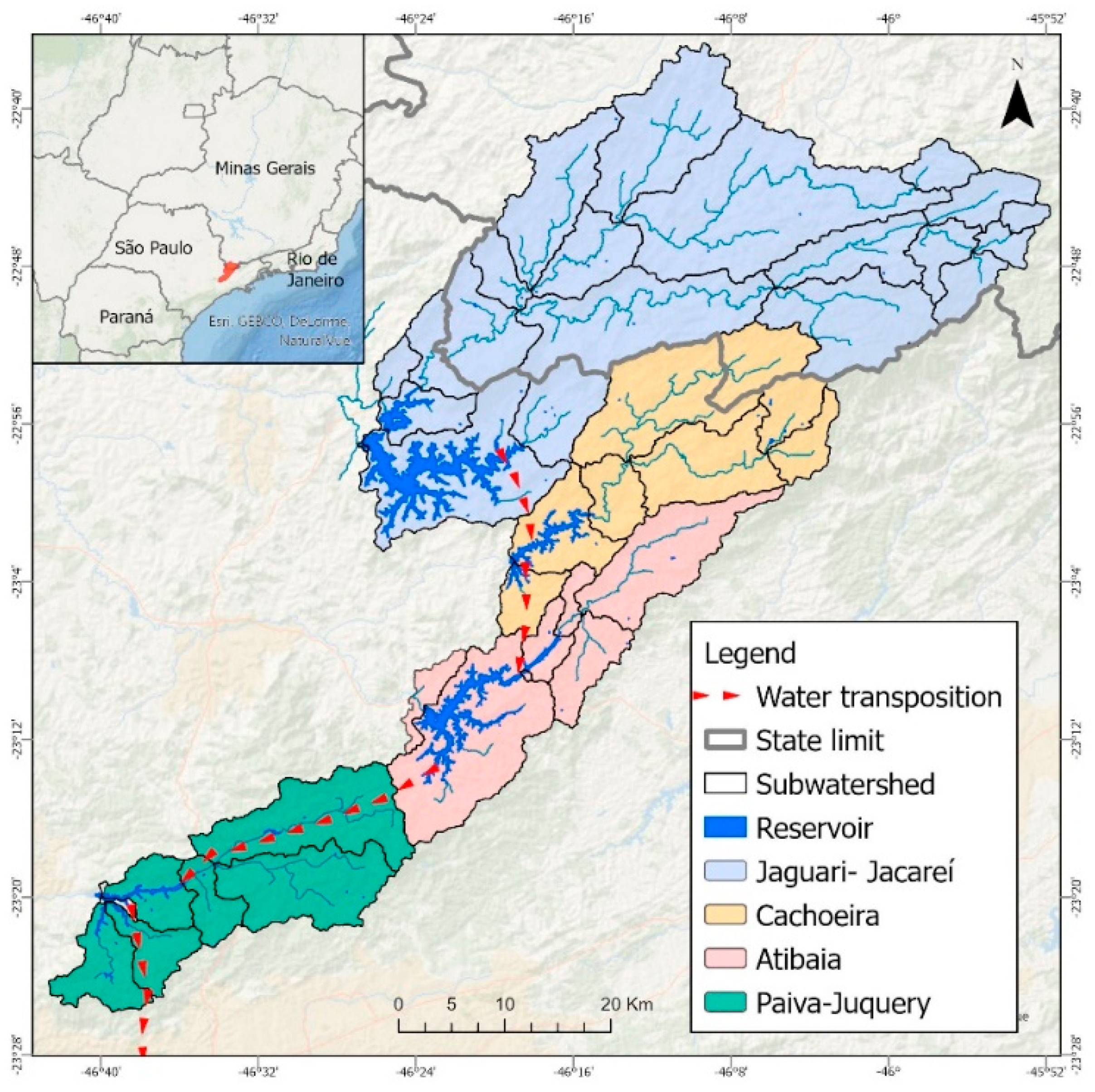
The Sao Paulo Cantareira water supply system (CWSS), which comprises the Jaguari/Jacareí, Cachoeira, Atibainha, Paiva Castro, and Aguas Claras reservoirs, began operations in 1974, with a storage capacity of 1.49 billion m
3, supplying approximately 9 million inhabitants of the Sao Paulo Metropolitan Region (SPMR) [
3]. The production capacity of its water treatment plant ETA Guarau is 33 m
3/s, meeting around 47% of the demand of the SPMR and 65% of the demand of the municipality of São Paulo. In October 2014, the lowest inflow on record (i.e., since 1930) was registered, reaching 5.2 m
3/s [
3]. Mean discharge in the summer of 2014 was 17.9 m
3/s, and in 2015 it was 24.0 m
3/s: 70% and 60%, respectively, below the average 1930–2013 summer discharge of 59.8 m
3/s [
4]. Storage levels were as low as 5% of system capacity in January 2015 and 15% at the end of the rainy season in March 2015. This episode is an example of increased vulnerability to climate change due to human-caused increases in temperature, where the socioeconomic-political situation, including larger water demand for a growing population, may have aggravated the situation, generating an acute water crisis [
4].
Land-use changes—from forest to farmland, for example, and from farmland to urban settlements—impact watershed hydrology, including flow regulation [
5]. Considering the complexity of the relationship between forests and rainfall and the regulation of climate in South America, mitigating droughts requires co-ordinated efforts to stop deforestation and restore deforested areas in different regions [
6]. Furthermore, markets fail to reflect the full economic value of the hydrologic services provided by natural watershed lands, which leads to the loss of watershed hydrologic services and the benefits they deliver to people [
7]. For example, Postel and Thompson (2005) [
5] pointed out that conserving and restoring the watershed of the Catskill mountains that supplies New York City’s drinking water via a USD 1.5 billion investment could avoid USD 4.5–6.5 billion in costs of engineering-based solutions such as a filtration plant. In this sense, the conservation and restoration of watersheds are essential for making water supplies more resilient, with nature-based solutions (NbS) or green infrastructure emerging as an important option for water security policies [
8]. Extreme drought events can result in high economic costs, which may be reduced by strategic investments in NbS. Since the benefits of drought mitigation programs can be approximated as the avoided cost of water shortages, the development of methodologies for quantifying the cost of drought is important [
9].
Many studies have estimated the economic costs of drought [
10,
11,
12,
13]. Dolan et al. (2021) [
10] applied a global-to-basin-scale exploratory analysis of potential water scarcity impacts by linking a global human–Earth system model, a global hydrologic model, and a metric for the reduction in economic surplus (the sum of the producer and consumer surplus) due to resource shortages. Economic surplus is a measure of the net value added, or societal welfare gained due to economic activity, so the change in economic surplus is a useful metric because it captures how the impact of resource scarcity propagates across sectors and regions that depend on that resource [
10]. The losses caused by drought include household welfare losses due to restricted water use and reduced water quality, lost profits for companies due to forced slowdown or shutdown, and the costs associated with emergency supplies, revenue losses, and the increased monitoring and treatment for water suppliers [
9].
Several studies have assessed the drought faced by the State of Sao Paulo from 2014–2015. Some of these analyzed the extent of the drought and the connections between climate and hydrology [
4,
14]. Others identified the causes of the resulting water supply crisis and possible solutions [
6] or evaluated the effectiveness of the drought response [
15,
16]. However, despite the relevance of this question, to our knowledge, no study has estimated the cost of the water supply crisis for the SPMR. In order to fill this gap and assess the economic rationale for investment in NbS as a drought resilience measure, this paper examines the economic cost of the drought to industry and to the water supply and sewage sectors and estimates the potential benefits of investments in NbS in the CWSS (
Figure 1).
Using the results of hydrological modelling analyses for the CWSS [
17], we assess the potential economic benefits of NbS investment using estimated avoided income losses from the 2014–2015 drought event. We then conduct a cost–benefit analysis (CBA) to assess the economic viability of NbS investments in CWSS. CBA is s standard project evaluation tool and can include impacts of projects that are not adequately captured in markets, including social or environmental impacts [
18].
2. Methods
Assessing the monetary benefits of a drought mitigation program requires quantifying the economic cost of a drought event and how much this cost would be reduced under the program [
9]. Logar and Bergh (2011) [
19] provide an overview of the methods for assessing different types of drought costs, distinguishing between direct, indirect, and intangible costs. Direct costs take the form of market impacts, such as losses in livestock or crop production or reductions in utility water sales. Indirect costs include increased unemployment or increases in the prices of goods and services. Intangible costs occur in the form of nonmarket impacts, such as inconvenience, hardship, or, in extreme cases, death from reduced water availability or quality, impact on wildlife populations that support human uses, loss of biodiversity, or loss of wetlands and the services they provide, among others.
Logar and Bergh [
19,
20] consider the gross domestic product (GDP: the market value of all final marketed goods and services sold in a country in a given year) as a useful economic metric for exploring the impact of a drought by comparing the GDP in a single drought year to that in the preceding, nondrought year. They point out that GDP has been used by the World Bank to study the relationship between a country’s economic structure and its sensitivity to drought to enable the incorporation of drought shocks into economic and development planning and to suggest structural adjustment programs to reduce drought vulnerability.
GDP equals the sum of the gross value added (GVA) from all goods and services at basic prices, plus taxes and minus subsidies. GVA is defined as the value of total output (at basic prices) net of inputs (valued at producer prices). GVA net of consumption of fixed capital (i.e., depreciation) yields net value added (NVA). NVA arguably is a preferred measure of value-added because depreciation may be considered a production cost. However, data on depreciation are not always available. Because both GVA and NVA measure total value added, we choose, based on data availability, one or the other of these metrics to estimate the cost of drought. Specifically, we use the GVA of the industrial sector in the municipalities of the CWSS and the net value added (NVA) of the municipal water supply and sewage company (SABESP), for which data on depreciation and amortization were available.
The drought impact assessment considered two discrete impacts and two groups of municipalities. The first is the economic impact on industry in all municipalities in the CWSS, which includes eight cities: Bragança Paulista, Caieiras, Franco da Rocha, Joanópolis, Mairiporã, Nazaré Paulista, Piracaia, and Vargem. The second is the economic impact on water supply and sewage services in all municipalities served by the CWSS, which include Caieiras, Francisco Morato, Franco da Rocha Guarulhos, Osasco, Santo André, São Caetano do Sul, and São Paulo. Since some of these municipalities are also supplied by other water supply systems, each municipality has a different percentage of dependence on water supplied from the CWSS. To assess the drought impact on water supply and sewage services (henceforth: water sector) by municipality, we calculated the coefficient of dependence on the CWSS, which is defined in the State Water Resources Plan 2020–2023 [
21] (
Table 1).
Our analysis is limited to the direct impact on the industrial and water sectors because the quantification of other drought costs was beyond our scope and would require separate analyses. Particularly important among these are the impacts on the agricultural sector and on household welfare (from restrictions on water supply or increased water prices, especially for vulnerable individuals).
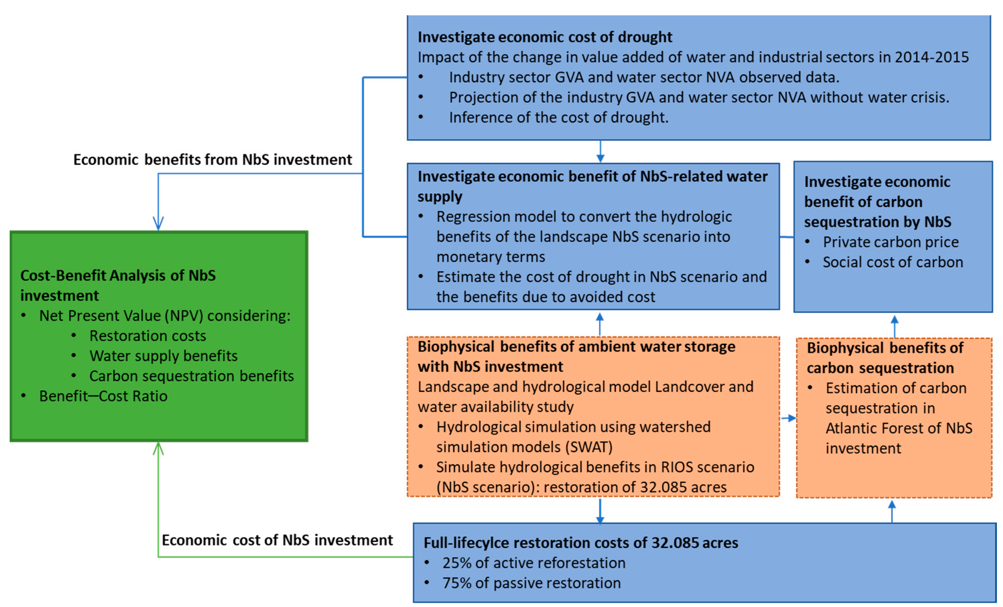
Figure 2 summarizes the different steps of the methods described in this section.
2.1. Economic Cost of Drought for Water and Industrial Sectors
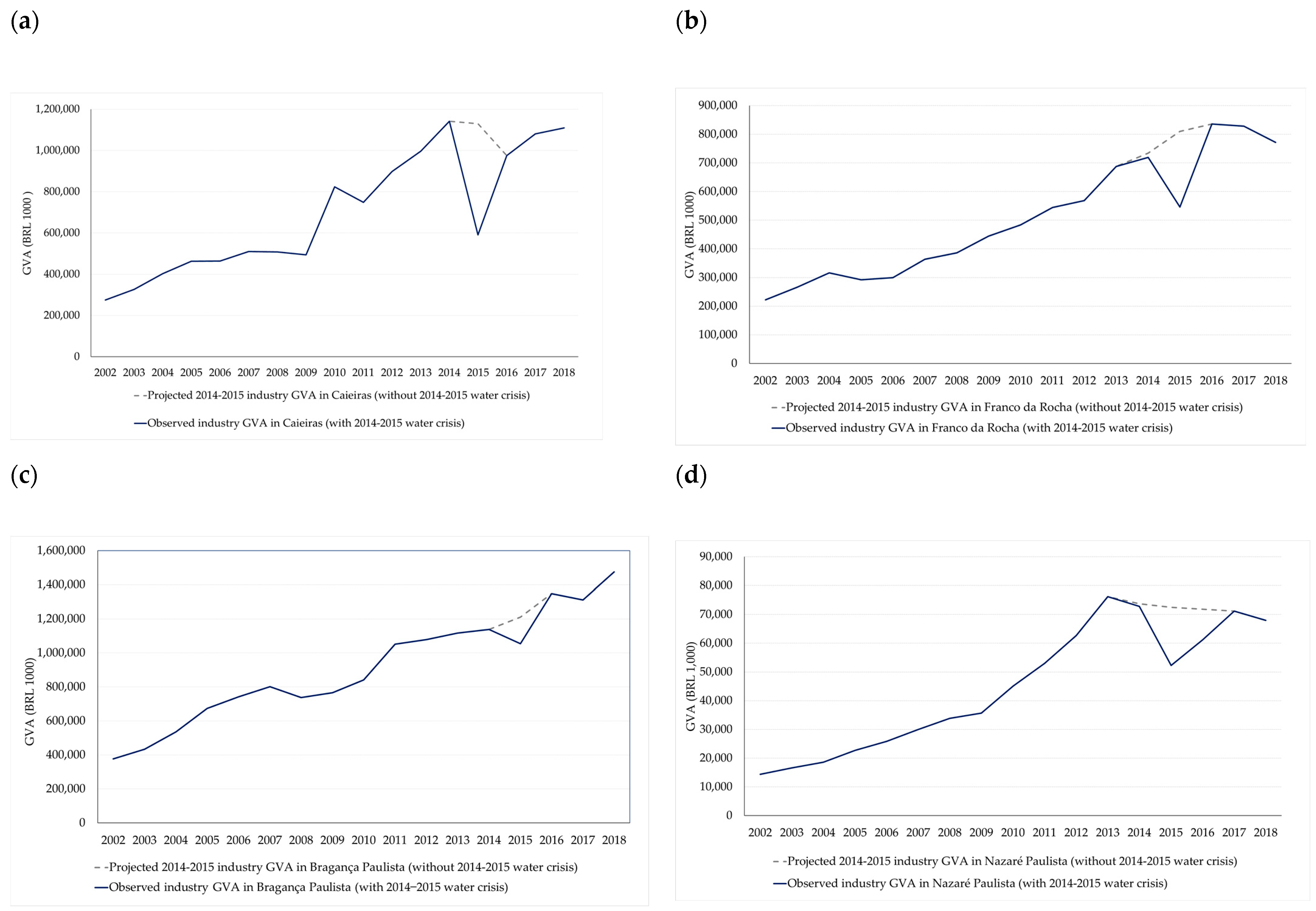
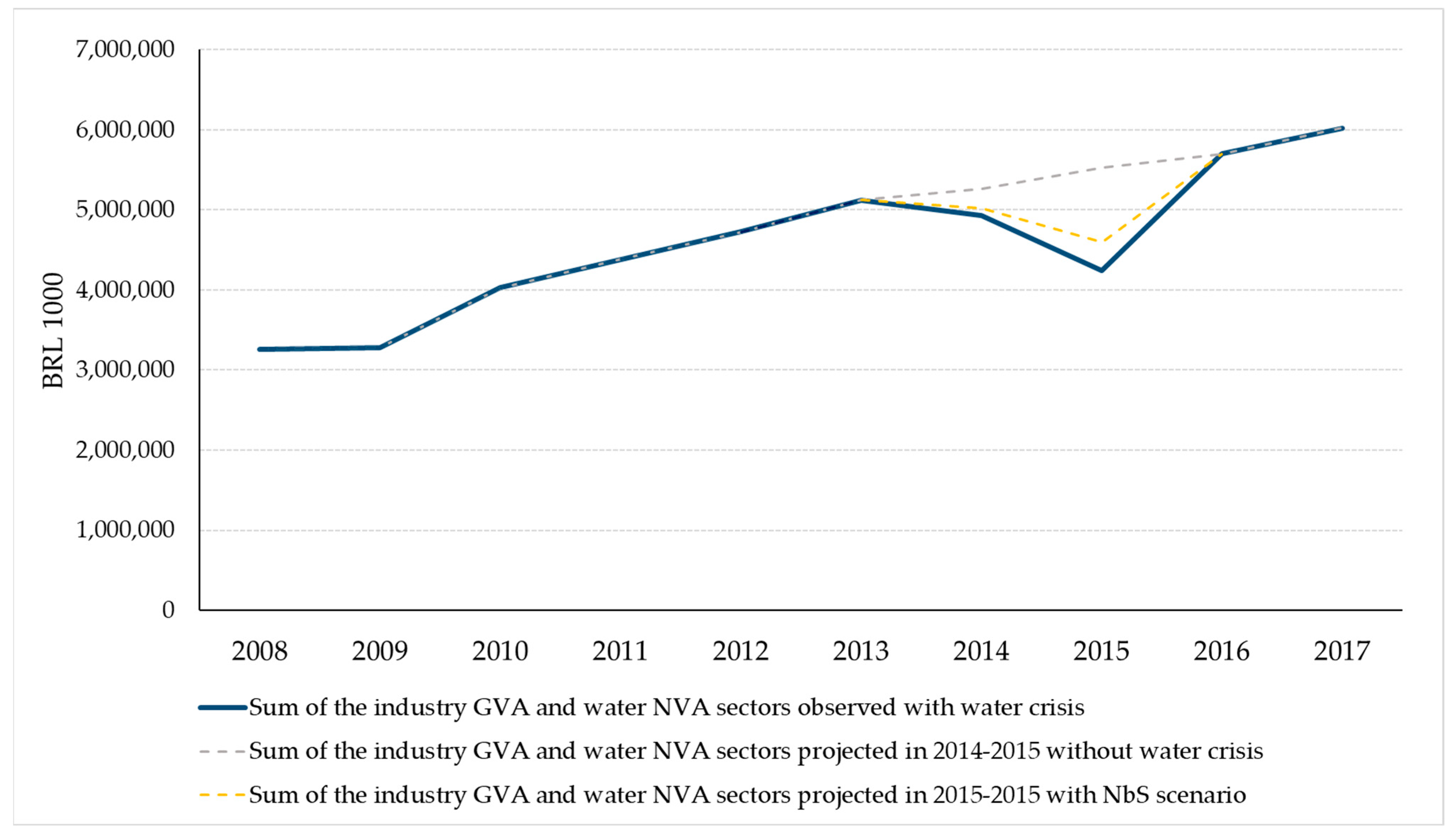
To estimate the potential economic benefits of an NbS scenario, we estimate how much hypothetical earlier NbS investments could have reduced the economic losses experienced by the industrial sector and the water sector during the 2014–2015 CWSS water crisis.
In this counterfactual approach, we estimate what the industrial GVA and water sector NVA would have been in 2014–2015 under a hypothetical scenario of earlier NbS investment in natural infrastructure in the CWSS source watersheds. The counterfactual scenario is constructed based on a regression analysis of the 2002–2013 trend in industrial GVA and the 2008–2013 trend in water sector NVA. In the analysis of industrial GVA, we are controlling for the 2014–2015 fluctuation in industrial GVA in the larger surrounding great Sao Paulo Metropolitan Region outside of the CWSS that was not directly affected by the water crisis in the CWSS. We use the estimated regression equations to construct the counterfactual industrial GVA and water sector NVA in 2014 and 2015, projecting both indicators’ performance in the hypothetical NbS scenario. The differences between the projected and the observed NVA and GVA data, respectively, provide an indication of the economic losses incurred by these two sectors as a result of the water crisis, that is, the drought cost (DC).
The drought cost for the industrial and water sectors was estimated as follows:
where:
: total drought cost; the sum of the value-added loss in the industrial (ind) and water sectors (ws); : drought-attributable cost in the water sector in year t; : drought-attributable cost in the industrial sector in year t;
observed water sector NVA in municipality i in year t.
projected water sector NVA in the NbS scenario in municipality i in year t.
: observed industrial GVA in municipality i in year t.
: projected industrial GVA in NbS scenario in municipality i in year t.
The projected and in 2014 and 2015 under the hypothetical NbS scenario were estimated using the trend equation of the observed variables until 2013, i.e., before the water crisis. The selection of the trend curve is determined by the regression equation with the highest coefficient of determination (R2), i.e., the one that minimizes the sum of squared residuals calculated from the regression by ordinary least squares (OLS).
2.1.1. Data for the Water Sector
For the analysis of the water sector, we obtained NVA data from SABESP’s Financial Statement Reports from 2008 to 2018 [
22]. However, the reports cover the entire company and include more than 300 municipalities to which SABESP provides water services. To estimate drought impacts on water sector NVA associated with the CWSS, we proceeded as follows. First, we checked that annual direct and indirect operating revenue (FN005—direct and indirect operating revenue: annual billed amount arising from the service provider’s core activities corresponding to the result of the sum of the direct operating revenue from water, sewage, exported water, imported sewage, and indirect operating revenue.) in the National Sanitation Information System (SNIS) [
23] and annual variable operation revenue reported in SABESP Financial Statements matched. We then calculated each municipality’s water sector NVA, as the product of a municipality’s ratio of water and sewage operational revenue, and SABESP’s overall NVA. Note that in doing so, we assumed that the net value added as a share of the total revenues is constant across SABESP operations in all municipalities.
2.1.2. Data for the Industrial Sector
The database used for the industrial GVA analysis included the municipal GDP for the period 2002 to 2018 and the industrial sector price index of the National Accounts System, both made available by the Brazilian Institute of Geography and Statistics (IBGE).
2.2. Economic Benefits of Ambient Water Storage with NbS Investment
The hypothetical NbS scenario used in our analysis and its modeled impact on the hydrologic behavior of the CWSS-sourced watersheds is presented in Acosta et al. (2023) [
17].
Table 2 shows the impact of the NbS scenario on the annual combined available surface flows (the sum of surface flows and groundwater-to-stream flows) in the CWSS, as estimated using the Soil and Water Assessment tool (SWAT). In all years, the NbS scenario shows increased flows when compared to the baseline scenario (38% or 178 hm
3 on average). The results generally (though not always) show proportionally larger modeled flow increases in years with lower flows. This is particularly true in the drought years of 2014 and 2015, with estimated flow increases of 45% in both years in the NbS scenario over the baseline scenario. This suggests that the adoption of NbS interventions in the CWSS-sourced watersheds increases the system’s resilience to drought.
We estimated two multiple linear regression equations for each of the industrial and water sectors. The first equation relates industrial GVA to water availability, capturing the dependence of industrial output on the water supply while controlling for broader economic fluctuations during the period (
Table 3):
where:
sum of water flow components–surface flows and groundwater to stream flows in hm3/year for the baseline scenario in Cantareira system from 2002 to 2017;
INDw: sum of industrial water withdrawal in CWSS municipalities (hm3/year) from Water National Agency data;
: sum of the industrial GVA of the municipalities of the São Paulo Metropolitan Region outside of the CWSS from IBGE.
: silviculture production in municipalities in Cantareira system (m3/year) from the annual survey PEVS (IBGE).
Specifically, we estimate industrial GVA (GVAind) in the CWSS as a dependent variable that is a function of surface flow and groundwater-to-stream flow (SURFGRDw), industrial water withdrawal (INDw), total industrial GVA of the larger São Paulo Metropolitan Region (GVAmrsp), and silviculture production volume (SILVp). The variable GVAmrsp allows us to control for the effect of broader economic fluctuations in industrial output on the industrial output of the CWSS area, while the variable SILVp allows us to control for the effect of regional wood production cycles on GVA, with wood being an intermediate input in the pulp and paper industry, which accounts for 60% of industrial GVA in the municipality of Caieiras.
Table 3.
Values of the dependent and explanatory variables used in the industrial GVA model regression.
Table 3.
Values of the dependent and explanatory variables used in the industrial GVA model regression.
| Year | Dependent Variable (Yi) | Explanatory Variables (Xij) |
|---|
| GVAind | INDw | SURFGRDw baseline | GVAmrsp | SILVp |
|---|
| 2002 | 999,451.96 | 7.20 | 15,783.62 | 50,361,745.17 | 290,011.00 |
| 2003 | 1,161,536.32 | 7.36 | 10,690.33 | 54,489,515.08 | 270,803.00 |
| 2004 | 1,433,094.80 | 8.15 | 14,157.30 | 66,018,997.08 | 268,079.00 |
| 2005 | 1,640,397.23 | 8.45 | 14,929.78 | 76,235,382.54 | 283,470.00 |
| 2006 | 1,724,987.58 | 21.24 | 14,964.53 | 77,864,795.20 | 272,870.00 |
| 2007 | 1,920,420.51 | 23.84 | 16,399.71 | 90,209,379.70 | 344,658.00 |
| 2008 | 1,880,731.97 | 23.95 | 21,935.15 | 91,746,062.37 | 387,026.00 |
| 2009 | 2,002,024.00 | 29.67 | 24,455.70 | 99,180,127.03 | 366,941.00 |
| 2010 | 2,518,056.23 | 33.24 | 25,451.59 | 111,930,774.15 | 450,379.00 |
| 2011 | 2,796,167.54 | 30.54 | 19,604.91 | 124,937,483.96 | 355,940.00 |
| 2012 | 2,982,877.86 | 32.75 | 14,121.48 | 125,553,381.84 | 342,601.00 |
| 2013 | 3,279,475.39 | 36.85 | 14,366.68 | 134,489,533.18 | 382,083.00 |
| 2014 | 3,450,474.92 | 37.95 | 2655.68 | 133,010,554.46 | 395,315.00 |
| 2015 | 2,624,585.95 | 40.71 | 8681.62 | 129,288,693.27 | 374,727.00 |
| 2016 | 3,619,894.67 | 40.61 | 20,281.30 | 126,438,875.01 | 545,070.00 |
| 2017 | 3,702,793.02 | 42.52 | 9875.78 | 126,930,105.06 | 543,031.00 |
The results show that the model is statistically significant at the 5% level (significance-F = 5.89771 × 10⁻⁸), as are the three independent variables: SURFGRDw (p-value = 0.0169 < α = 0.05), GVAmrsp (p-value = 0.0005 < α = 0.05), and SILVp (p-value = 0.0012 < α = 0.05).
In the second model, water sector NVA (
NVAws; from 2008 to 2017) is the dependent variable and is a function of the surface flow and groundwater-to-stream flow (
SURFGRDw), micromeasured water volume (
MICROw), and average water tariff (
TRFw), as per the equation below (
Table 4):
where:
sum of surface flow and groundwater-to-stream flow in CWSS in hm3/year for the baseline scenario from 2008 to 2017;
MICROw: annual water volume (measured by water meters) installed in the active water connections in São Paulo municipality (1000 m3/year) from the variable AG008 in SNIS;
: average of the water tariff applied for residential, commercial, and industrial use from 2007 to 2017 from the Arsesp Deliberation published annually in the Official Gazette of the State of São Paulo.
Table 4.
Values of the dependent and explanatory variables for the water sector NVA model regression.
Table 4.
Values of the dependent and explanatory variables for the water sector NVA model regression.
| Year | Dependent Variable (Yi) | Explanatory Variables (Xij) |
|---|
| NVAwr (BRL 1.000) | MICROw | SURFGRDwbaseline | TRFw |
|---|
| 2008 | 1,380,085 | 299,419.94 | 21,935.15 | 7.39 |
| 2009 | 1,281,392 | 303,991.88 | 24,455.70 | 7.76 |
| 2010 | 1,510,585 | 314,061.26 | 25,451.59 | 8.07 |
| 2011 | 1,583,303 | 321,777.02 | 19,604.91 | 8.63 |
| 2012 | 1,745,023 | 327,793.62 | 14,121.48 | 9.07 |
| 2013 | 1,844,663 | 331,348.62 | 14,366.68 | 9.57 |
| 2014 | 1,478,490 | 303,576.47 | 2655.68 | 10.20 |
| 2015 | 1,617,500 | 261,359.58 | 8681.62 | 11.75 |
| 2016 | 2,076,777 | 277,097.54 | 20,281.30 | 12.74 |
| 2017 | 2,318,296 | 288,357.75 | 9875.78 | 13.75 |
The second model is also statistically significant at the 5% level (significance-F = 0.0003), as are the three explanatory variables: SURFGRDw (p-value = 0.0266 < α = 0.05), MICROw (p-value = 0.0034 < α = 0.05), and TRFw (p-value = 0.000069 < α = 0.05).
The regressions were performed for the baseline scenario to obtain the coefficients that relate the independent and dependent variables. The regression equations were used to estimate the industrial GVA and water sector NVA for the years 2014 and 2015 under the NbS scenario using the surface and groundwater flows (
SURFGRWDw) of the NbS scenario for those years (
Table 2).
2.3. Cost–Benefit Analysis of NbS Investment
Our CBA of NbS investment in the CWSS considered the estimated full-lifecycle costs of the NbS intervention scenario, specifically, of restoring 32,085 hectares distributed across the four subwatersheds [
17], as well as the value of increased water availability for the industrial and water sectors, and carbon sequestration. As discussed previously, other benefits were beyond the scope of our CBA. The full-lifecycle costs of the program and the three economic benefit scenarios using a 35-year time horizon are as follows:
- I.
Scenario 1: Value of increased water supply from NbS interventions, estimated using the modeled cost of the water crisis and assuming a drought recurrence interval of 10 years. This scenario assesses the private financial viability of investments in the NbS interventions purely on the basis of reduced water scarcity (i.e., increased flows) in the industrial and water sectors during drought years and of the cost of the NbS interventions;
- II.
Scenario 2: Same as Scenario 1 but including the potential revenues from the sale of certified carbon offsets on voluntary carbon markets, using a carbon offset price of USD 7.69/tCO
2 [
24] and assuming the offsets are issued every 5 years for carbon accumulated to date over a period of 35 years;
- III.
Scenario 3: Same as Scenario 1 but including the value of the avoided damages in Brazil from carbon sequestration as a result of the NbS interventions using a social cost of carbon for Brazil of USD 24/tCO
2 [
25]. This scenario assesses the economic viability of investments in NbS interventions on the basis of the sum of the financial value of reduced water scarcity (i.e., increased flows) in the industrial and water sectors during drought years and the societal value from avoided climate damages attributable to the NbS interventions.
2.3.1. Full-Lifecycle Restoration Costs
We estimated the cost of restoration interventions using two restoration techniques commonly implemented in Brazil’s Atlantic Forest biome:
Active reforestation: Native Forest restoration through the removal of forest-degrading uses, such as cattle grazing (via fencing), the control of exotic plant species, and the planting of seedlings to mimic and accelerate the natural regeneration process. This restoration technique was assumed to account for 25% of the NbS intervention area;
Passive restoration: Restoration of degraded forest areas through the removal of forest-degrading uses, such as cattle grazing (via fencing), the control of exotic plant species, and seedling enrichment as-needed during the natural regeneration process. This restoration technique was assumed to account for 75% of the NbS intervention area.
We obtained unit costs from the literature [
26] for the individual activities involved in each of the two intervention techniques. These unit costs were reviewed and validated with local implementation partners who have been working with TNC in the CWSS region since 2009 to update them to current prices. We used these unit costs to generate annual restoration cost estimates. These costs were then categorized into ‘direct implementation costs’ (labor and materials in the first year of implementation), ‘maintenance costs’ (follow-up labor and materials required for intervention upkeep), ‘opportunity costs’ (payments to landowners for hosting the intervention), ‘transaction costs’ (outreach costs incurred to organize the green infrastructure, including landowner mobilization and engagement, contract development, and compliance monitoring) and ‘program management costs’ (assumes personnel including program director, monitoring & evaluation manager and implementation manager, and the amounts for overhead and equipment) [
27]. The full-lifecycle per-hectare average cost estimated for passive restoration is BRL 22,700 ha
−1, and for active restoration is BRL 34,980 ha
−1 at current (2021) prices.
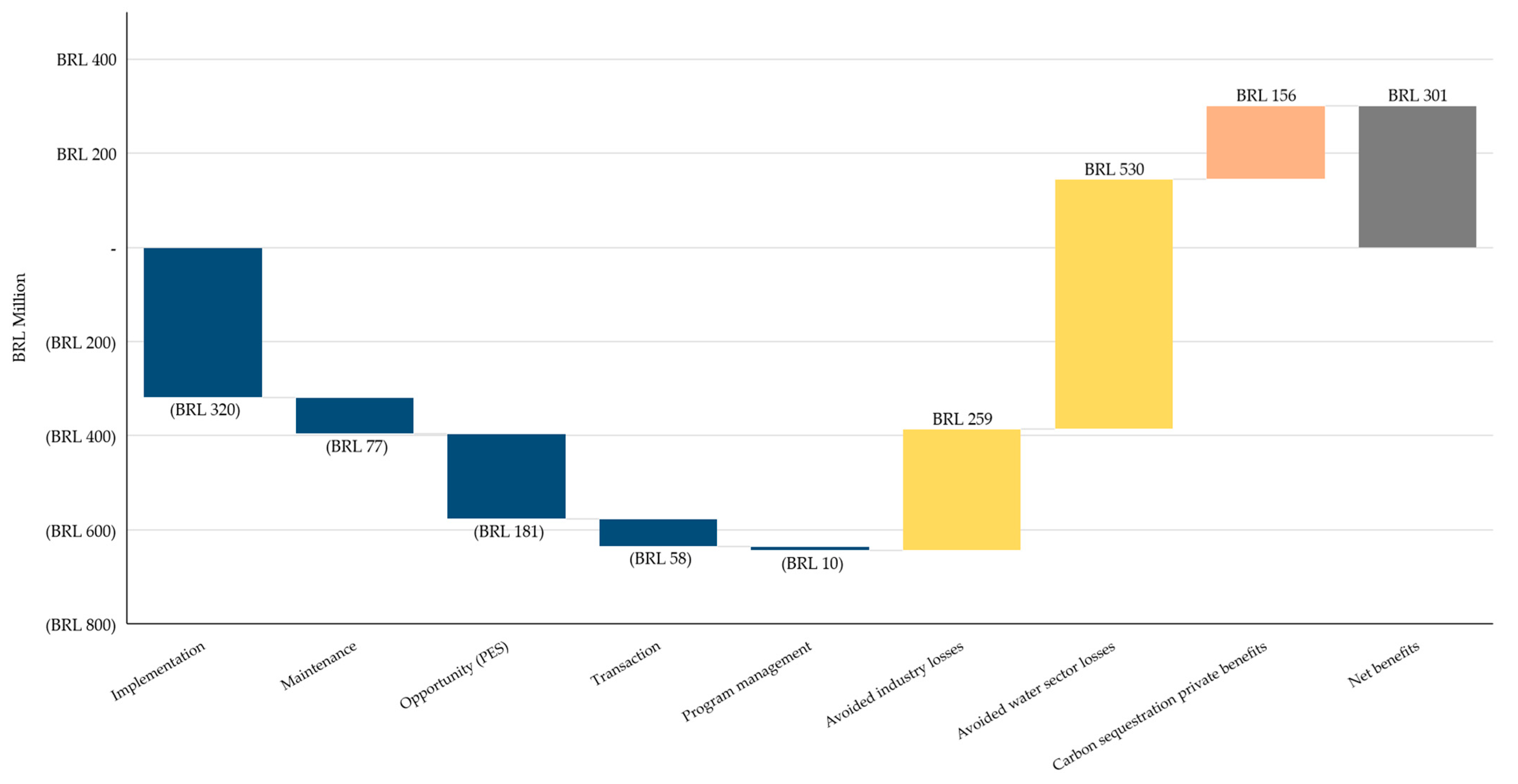
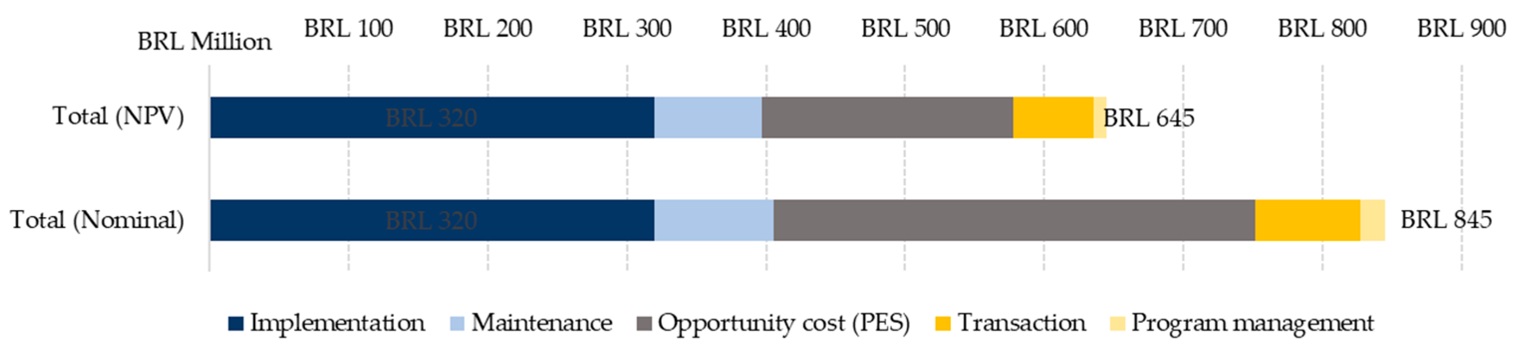
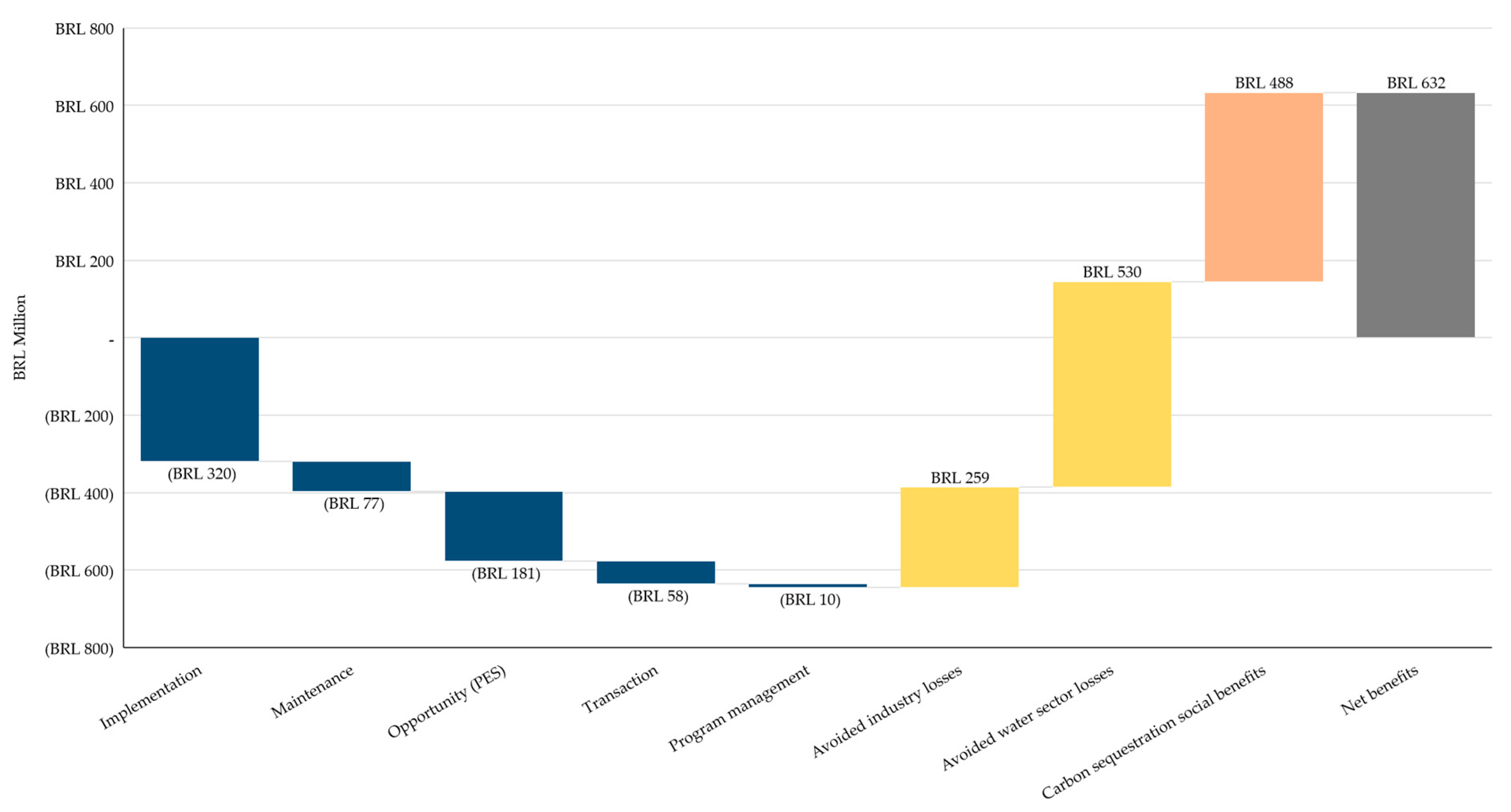
Total lifecycle (35 years) costs of the NbS scenario and their breakdown into cost categories are presented in
Figure 3. Total estimated program cost is BRL 845 million in nominal terms (at 2022 prices) or BRL 645 million in net present value (NPV) terms using the 4.36% social discount rate (SDR) estimated for Brazil by Moore et al. (2020) [
28]. In Brazil, investments in watershed NbSs are primarily financed by public or quasipublic entities and, thus, constitute long-lived environmental projects that should be evaluated using SDRs [
29]. The rate we use exceeds the 3.45% Ramsey SDR estimated for Brazil by Addicott et al. (2020) [
30]. It also exceeds the 3% and 2% median risk-free SDRs reported in large surveys of academic economists [
31] and discounting experts [
32], respectively, which were not specific to Brazil. All else being equal, our choice of discount rate is conservative because our estimated NbS benefits and ROI of NbS investments are inversely related to the size of the discount rate.
2.3.2. Lifecycle Water Supply Benefits
Estimating lifecycle program benefits for the NbS scenario requires extending the water supply benefits during drought years (
Table 2) over the scenario’s full 35-year lifecycle. Three steps are used to implement this generalization:
Inflation adjustment: Relying on the IPCA inflation rate from IBGE (
https://www3.bcb.gov.br/ (accessed on 1 March 2022)) and a consumer price index of 37.5%, we adjusted the BRL 443.9 million in 2015 avoided losses for the NbS scenario to current prices (2021), yielding BRL 610.0 million;
Drought incidence period: We assume a ‘drought recurrence period’ to reflect the likelihood (in any given year) of the occurrence of drought-related damages equivalent to those from 2014–2015. Our base assumption is a 1 in 10-year incidence factor, meaning we assume losses equivalent to those experienced in 2015 will occur once in every ten-year period;
Benefits realization curve: Green infrastructure interventions–particularly those involving ecosystem restoration, such as the reforestation techniques used in the NbS scenario–require time to develop their full hydrologic functionality and generate related water security outcomes. We assume that the benefits from ecosystem restoration follow a sigmoid function (logistic or ‘S’ curve) over a predefined number of years. TNC field practitioners and implementation partners in the CWSS generally witness full ecosystem benefit generation by year 8 in the case of active restoration and by year 12 in the case of passive regeneration; when using the aforementioned assumed split of 75% passive regeneration and 25% active reforestation, this implies that full hydrologic service delivery will be achieved in year 11.
2.3.3. Carbon Sequestration Benefits
Beyond water security outcomes, the NbS interventions analyzed in this study are anticipated to generate cobenefits that include reductions in atmospheric carbon through forest restoration. The NbS interventions focus on areas that are not legally protected and are currently used for extensive cattle grazing, thus fulfilling the additionality criterion of carbon offset protocols. Carbon sequestration was quantified using a systematic qualitative and quantitative literature review of 166 studies conducted in Atlantic Forest passive and active restoration sites. By compiling information on biomass, age, climate, slope, forest type, and past land use, carbon sequestration was estimated using forest growth patterns.
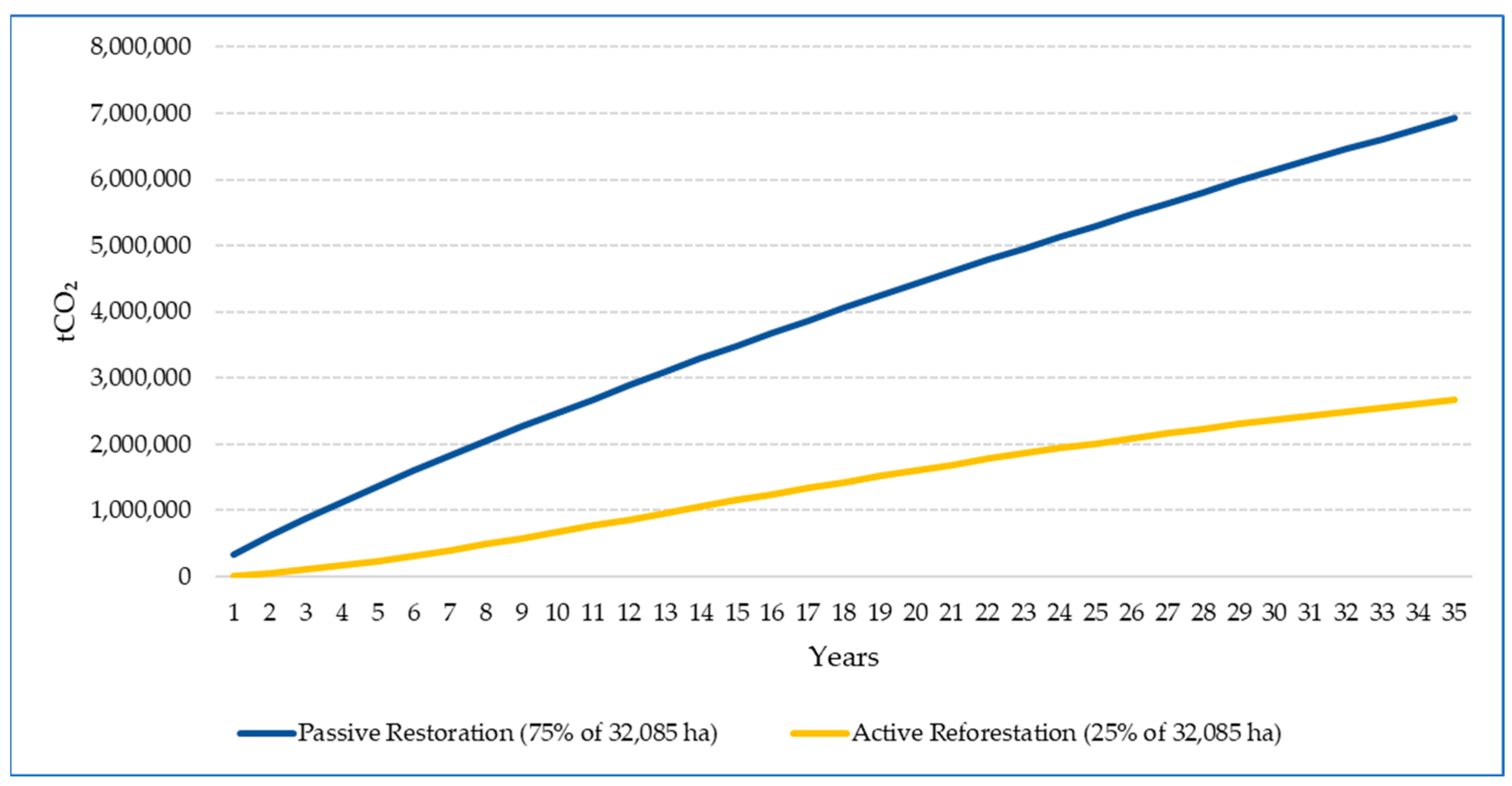
Figure 4 presents the cumulative carbon sequestration for passive and active restoration over the 35-year analysis life cycle. The restoration of 24,064 hectares via passive reforestation and 8021 hectares via active restoration is estimated to achieve a sequestration of 6.92 million and 2.67 million tons of CO
2, respectively, for a total of 9.59 million tCO
2. The certification and commercialization process requires the inclusion of the risks associated with the maintenance and permanence of the project, the leakage of deforestation to other areas, and the uncertainty in the verification and commercialization process also called the buffer factor. For this analysis, we assume a conservative 30% buffer factor, thus resulting in a potential creditable carbon sequestration of 6.71 million tCO
2.
The economic value of net carbon sequestration in NbS scenarios can be evaluated from a private financial perspective or from a social welfare perspective. The first uses the potential revenue of landowners or that the project could realize from the sale of carbon credits, which is the product of the estimated net offset volume the project would generate (e.g., net of the required buffer quantity) and the price of the offsets in the markets the project would be able to access (e.g., [
33]). To estimate this potential revenue, we use the average price of USD 7.69/tCO
2, which, in 2020, was the average price paid for reforestation and afforestation projects on voluntary carbon markets [
24].
The social welfare approach considers the benefits society as a whole would receive in the form of avoided damages from higher atmospheric CO
2 levels, which the NbS scenario reduces via its carbon sequestration impact. This approach values the carbon using estimates of the social cost of carbon (SCC), which indicates, for a given year, the sum of the discounted future economic costs associated with future climate-related damages caused by the emission of one additional ton of carbon dioxide [
25,
34].
The most recent mean estimates of the SCC (or, more precisely, the SCCO
2) are USD 185 tCO
2−1 ([
35]; in 2020 USD) and USD 307 tCO
2−1 ([
36]; in 2015 USD), respectively. Both represent global climate damages which, for a variety of reasons, are widely considered appropriate even for use in domestic policy analyses (e.g., Interagency Working Group [IWG] on Social Cost of Greenhouse Gases, 2021 [
37]). In our analysis, we instead used Ricke et al.’s (2018) [
25] country-level SCC for Brazil, which is USD 24/tCO
2, reflecting the mean value of the discounted future expected damages
only in Brazil (rather than in the world as a whole) from one additional ton of CO
2 emissions. Furthermore, while the SCC increases over time (e.g., [
37,
38]), we use a constant SCC value. Both choices impart a conservative bias in our estimates. Because of the sensitivity of the results to the exchange rate and the substantial interannual volatility of the BRL/USD exchange rate, we used the average 2012–2022 exchange rate of BRL 3.58/USD (Brazil Central Bank, 2022) to convert the USD–denominated SCC value to BRL.
4. Discussion
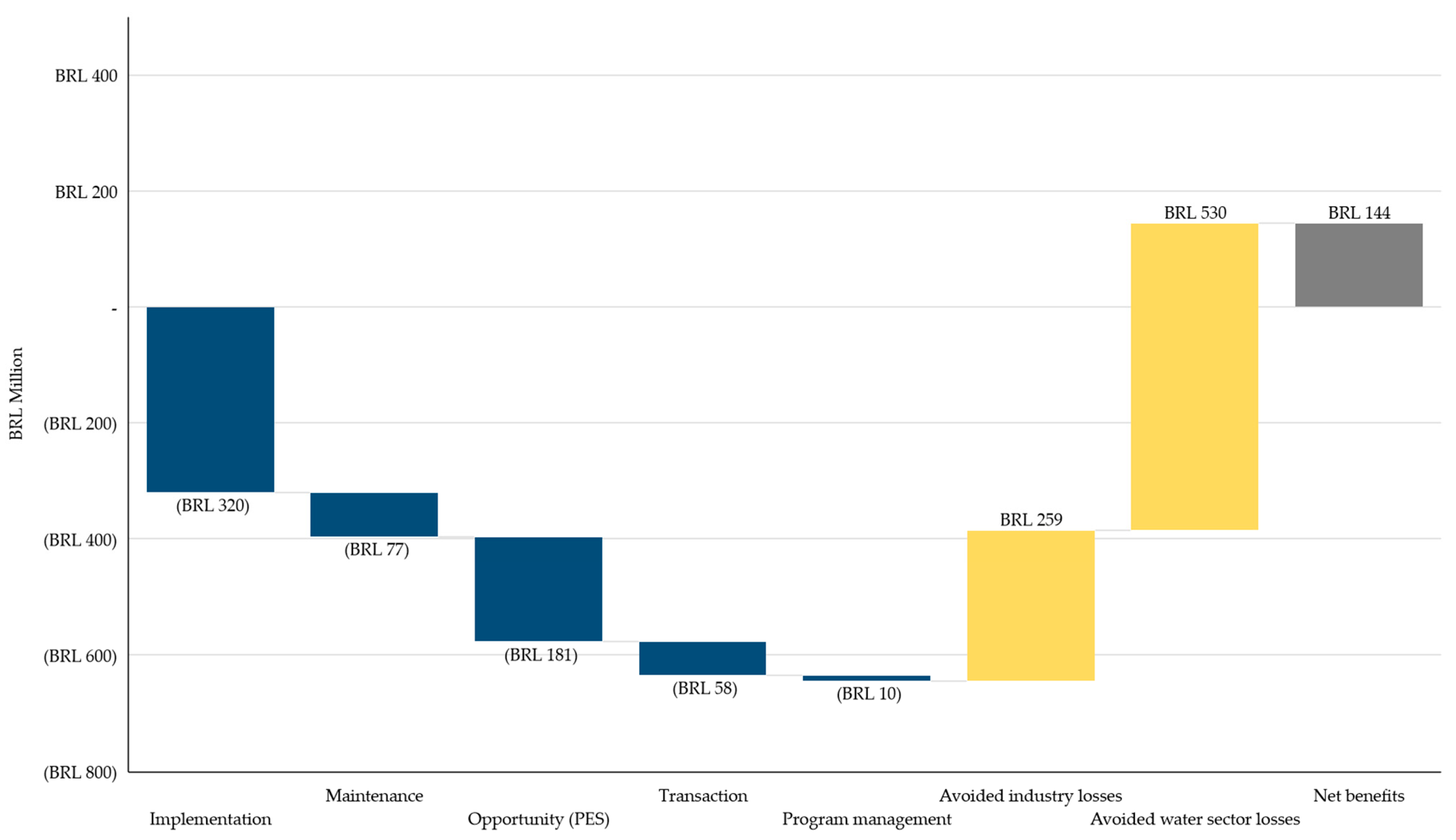
This study focuses on two specific benefits of investing in NbS in the CWSS source watersheds: improved water availability for the industrial and water sectors under drought conditions, and increased carbon sequestration. The NbS scenario involves 32,085 ha of forest restoration implemented via a mixture of passive and active restoration techniques. Assuming a 1-in-10-year incidence factor (i.e., drought-related economic losses equivalent to those incurred during the 2014–2015 water crisis occur once every 10 years) and using a 35-year analysis time horizon with full lifecycle cost accounting for the NbS interventions, we find that the NbS investment scenario passes a cost–benefit test even without including the value of the sequestered carbon.
However, the NbS scenario would be expected to generate additional important water security benefits. These include improved water quality from reduced sediment loading and the associated reductions in turbidity or reduced bacterial loadings from livestock waste entering the surface waters. Reduced turbidity in municipal source water can lower treatment costs [
39], while reduced bacterial contamination can lower water treatment costs and may avoid negative downstream human or livestock health impacts [
40]. Additionally, NbS interventions would positively impact biodiversity in the Atlantic Forest biome by restoring native forest cover in a system characterized by a high degree of endemism that has lost nearly 90 percent of its historic forest extent [
41].
We believe that our estimates of the benefits and economic value of NbS investments in the CWSS source watersheds are conservative due to our choice of parameter values for several key assumptions (e.g., discount rate and lag-time in NbS hydrologic functionality), but above all because our analysis excludes the benefits to households from the avoided water restrictions, as well as the avoided water treatment costs and health benefits from reduced turbidity and fecal coliform contamination in municipal source water.
While the positive benefit–cost ratios of the hypothetical NbS interventions indicate that the analyzed hypothetical BRL 645 million investment in NbS would have been justifiable both on narrow, private financial, as well as broader economic grounds, a key question is whether the NbS interventions would have been cost-competitive with alternative approaches to improving water security in the CWSS that can provide comparable benefits. That question is impossible to answer definitively without further analysis. A cursory comparison with SABESP grey infrastructure investments during and immediately after the 2014–2015 water crisis can provide a starting point. In 2015, the utility made a BRL 540 million investment in water transposition from the Jaguari Reservoir (Paraíba do Sul River) to the Atibainha Reservoir (Cantareira System), a BRL 29 million investment in the Guaió System to increase water supply in the Alto Tietê System by 1 m
3s
−1, and a BRL 132 million investment in the integration of the Rio Grande (Billings dam) with the Alto Tietê Water System (Taiaçupeba). Without knowing whether the water security impacts of these grey investments are similar in size and timing to those of the analyzed hypothetical NbS scenario, a comparison of the cost-effectiveness of the NbS and grey alternatives is not possible. Nevertheless, as interesting as this question is, in all likelihood, both natural capital and engineering solutions will be required to provide water security in a cost-effective manner, not just in the Sao Paulo area but in Brazil more broadly and indeed in many other parts of the globe [
8].


 ,
, 