Combining Hydrological Modeling and Regional Climate Projections to Assess the Climate Change Impact on the Water Resources of Dam Reservoirs

Abstract

Climate change may significantly impact the availability and quality of water resources in dam reservoirs by potentially altering the hydrological regime of lake tributaries and the corresponding flow–duration curves. Hydrological models driven by climate projections (downscaled to the watershed scale and bias corrected to eliminate systematic errors) are effective tools for assessing this potential impact. To assess the uncertainty in future water resource availability, resulting from the inherent uncertainty in climate model projections, an ensemble of climate models and different climate scenarios can be considered. The reliability and effectiveness of this approach were illustrated by analyzing the potential impact of climate change on the water availability at Brugneto Lake in northern Italy. This analysis was based on climate projections derived from an ensemble of 13 combinations of General Circulation Models and Regional Climate Models under two distinct scenarios (RCP4.5 and RCP8.5). The semi-distributed HEC-HMS model was adopted to simulate the hydrological response of the basin upstream of the lake. The hydrological model parameters were calibrated automatically via the PEST software package using the inflows to the lake, estimated through a reverse level pool routing method, as observed values. Future water availability was predicted for short- (2010–2039), medium- (2040–2069), and long-term (2070–2099) periods. The results indicate that the uncertainty in reservoir inflow is primarily due to the uncertainty in future rainfall. A moderate reduction in water availability is expected for Brugneto Lake by the end of the current century, accompanied by modifications in the flow regime. These changes should be considered when planning future adaptation measures and adjusting reservoir management rules.

1. Introduction

Global warming is having a tremendous impact on the Earth’s hydrological cycle, with significant social and economic consequences. The hydrological cycle shows changes, detectable since the mid-20th century, which are expected to be exacerbated in the future at both the global and regional scales, with different impacts at the catchment scale. In particular, droughts have increased in the Mediterranean region and will intensify in the future, with potentially serious hydrological, agricultural, and ecological impacts. The expected changes in climate may also affect the availability and quality of water resources [1].

Artificial reservoirs created by dams may play a key role in adaptation strategies to climate change [2]. The Italian National Adaptation Strategy to Climate Change [3] identifies, among the various strategies to cope with droughts, an increase in the capacity of existing artificial reservoirs, thereby making it possible to plan multi-year management of the water resource, in combination with an optimized management of reservoir levels. For this reason, it becomes essential to evaluate the potential impact of climate change on the inflow to artificial reservoirs and, therefore, on the catchment areas upstream of them. As an example, climate change can alter the hydrological regime of a river, as well as the flow–duration curves [4], forcing dam managers to adapt the reservoir management rules used currently.

Hydrological models driven by climate projections are useful tools through which to obtain quantitative insights into potential future river flow conditions (e.g., [5,6]). Indeed, hydrological models can effectively simulate the rainfall–runoff process and other dominant hydrological processes in watersheds with varying levels of detail, involving empirically, conceptually, or physically based models [7,8]. On the other hand, climate models provide future projections of several variables, including precipitation and temperature, which are key drivers of hydrological processes. These climate projections can be generated using different General Circulation Models (GCMs), which offer a coarse spatial resolution, or Regional Climate Models (RCMs), which provide a finer spatial resolution. The Intergovernmental Panel on Climate Change (IPCC) has selected different emission pathways (or scenarios), such as the Representative Concentration Pathways (RCPs) [9] and the Shared Socioeconomic Pathways (SSPs) [10], to depict possible alternative future conditions.

When conducting analyses on a local scale or within small watersheds to assess hydrological impacts, further refinement of the regional climate projections through a downscaling process may be necessary. Additionally, it is crucial to apply bias-correction techniques to correct systematic errors affecting the projections deriving from climate models [11,12,13,14,15].

In order to cope with the inherent uncertainty in climate model projections, it is advantageous to use an ensemble of climate models, rather than relying on a single realization [12,13,16]. This ensemble approach should also incorporate different climate scenarios. Accordingly, the selected hydrological model must be run multiple times for different climate projections, thus obtaining a set of potential outcomes [5]. In some cases, an ensemble of hydrological models is employed to investigate the uncertainty associated with models of different structural complexities [17].

Numerous studies in the literature combine hydrological models with climate model projections to evaluate the effects of climate change on water resources at the river basin scale (e.g., [18,19,20,21,22,23]), some of these focusing on assessing water resource availability in rivers that flow into natural or artificial lakes (e.g., [24,25,26,27,28,29,30]).

Versini et al. [24] investigated the impacts of climate change on the Llobregat Basin in Spain, which includes three large dams. The HBV (Hydrologiska Byråns Vattenbalansavdelning) model was coupled with climate projections from GCMs (either statistically or dynamically downscaled and bias corrected) under two different scenarios (A2 and B1) [31]. A future decrease in water resources was predicted for the study area, with the extent of this decrease varying depending on the scenario and time period under consideration. Additionally, that study showed that drought periods are expected to become more frequent, despite the high level of uncertainty.

Emami and Koch [25] used the SWAT (Soil and Water Assessment Tool) hydrological model to examine water resources in the basin of the Zarrine River, a tributary of Lake Urmia (Iran). The hydrological model was driven by bias-corrected future climate data from two GCMs, one for precipitation and another for temperature, under the RCP2.6, RCP4.5, and RCP8.5 scenarios. The results indicate a projected reduction in inflow to the lake by 2029, primarily attributed to a decrease in precipitation.

Teklay et al. [26] investigated how climate change could affect streamflow and evapotranspiration in the Lake Tana Basin in Ethiopia. The SWAT model was coupled with bias-corrected high-resolution climate projections, obtained from a single climate model under the RCP4.5 and RCP8.5 scenarios. Despite the predicted rise in temperature potentially leading to increased evapotranspiration, the expected increase in precipitation may result in higher streamflow levels by 2045–2055. The authors predicted a 7.2% increase in streamflow levels for the RCP4.5 scenario and a 33% increase for the RCP8.5 one, compared to 2005–2015.

Babur et al. [27] assessed the climate change impact on the reservoir inflow of Mangla Dam in Pakistan. The authors used climate projections from seven GCMs under the RCP4.5 and RCP8.5 scenarios in combination with the SWAT model. The Mangla Basin is likely to experience more frequent floods and fewer droughts in the future, due to the expected increases in both high and low flows.

D’Oria et al. [28] investigated the potential impacts of climate change on water resources within a watershed in northern Tuscany, Italy, which includes 19 dams. The authors combined the HEC-HMS (Hydrologic Engineering Center’s Hydrologic Modeling System) hydrological model with an ensemble of climate models under the RCP4.5 and RCP8.5 scenarios. A moderate reduction in water resources is expected for the study area during the medium- (2031–2040) and long-term (2051–2060) periods. The study showed that the presence of dams, with their storage capacities, serves to mitigate the impact of climate change, although the results strongly depend on the management strategies employed.

Abdulahi et al. [29] focused on the Upper Awash River Basin in Ethiopia to examine how climate change would impact future streamflow availability. They utilized the HBV hydrological model and incorporated bias-corrected climate projections from a single RCM for the RCP4.5 and RCP8.5 scenarios. The authors predicted an increase in the annual streamflow in the study area in the future.

Dau et al. [30] assessed water availability in the Huong River Basin in Central Vietnam, which includes three major reservoirs and is subject to climate and population changes. The HEC-HMS was used to simulate hydrological processes, while future climate variables under the RCP8.5 scenario were derived using two different approaches: one involved statistically downscaling GCM projections from a single model, and the other utilized bias-corrected RCM projections from a different model. Increases in both temperature and annual rainfall are expected for the future. Moreover, the results of the study led the authors to conclude that the Huong River Basin is likely to meet future water demands, even in the face of the most severe climate projections.

In this paper, we investigated the potential impacts of climate change on the inflow to Brugneto Lake, an artificial reservoir formed by Brugneto Dam, located in the province of Genoa, northern Italy. Climate projections from 13 RCMs of the EURO-CORDEX initiative [32] were downscaled and bias corrected for the study area, using available observed data. Daily precipitation and mean temperature data extending until the end of the current century were obtained under the RCP4.5 and RCP8.5 scenarios. This ensemble of climate projections was used to drive an HEC-HMS hydrological model calibrated for the watershed upstream of the dam, providing insights into water resource availability over short- (2010–2039), medium- (2040–2069), and long-term (2070–2099) periods. The use of a large ensemble of models and different scenarios increases the comprehensiveness and reliability of the climate projections, making it a novel and robust method for assessing future climate conditions in the study area.

This paper is structured as follows: Section 2 introduces the study area, presents the available climate data (including historical observations and future climate projections), outlines the hydrological data, and describes the implementation of the hydrological model. Section 3 presents the results, encompassing meteorological and hydrological data for historical and future periods. Finally, discussion and conclusions are reported in Section 4.

2. Materials and Methods

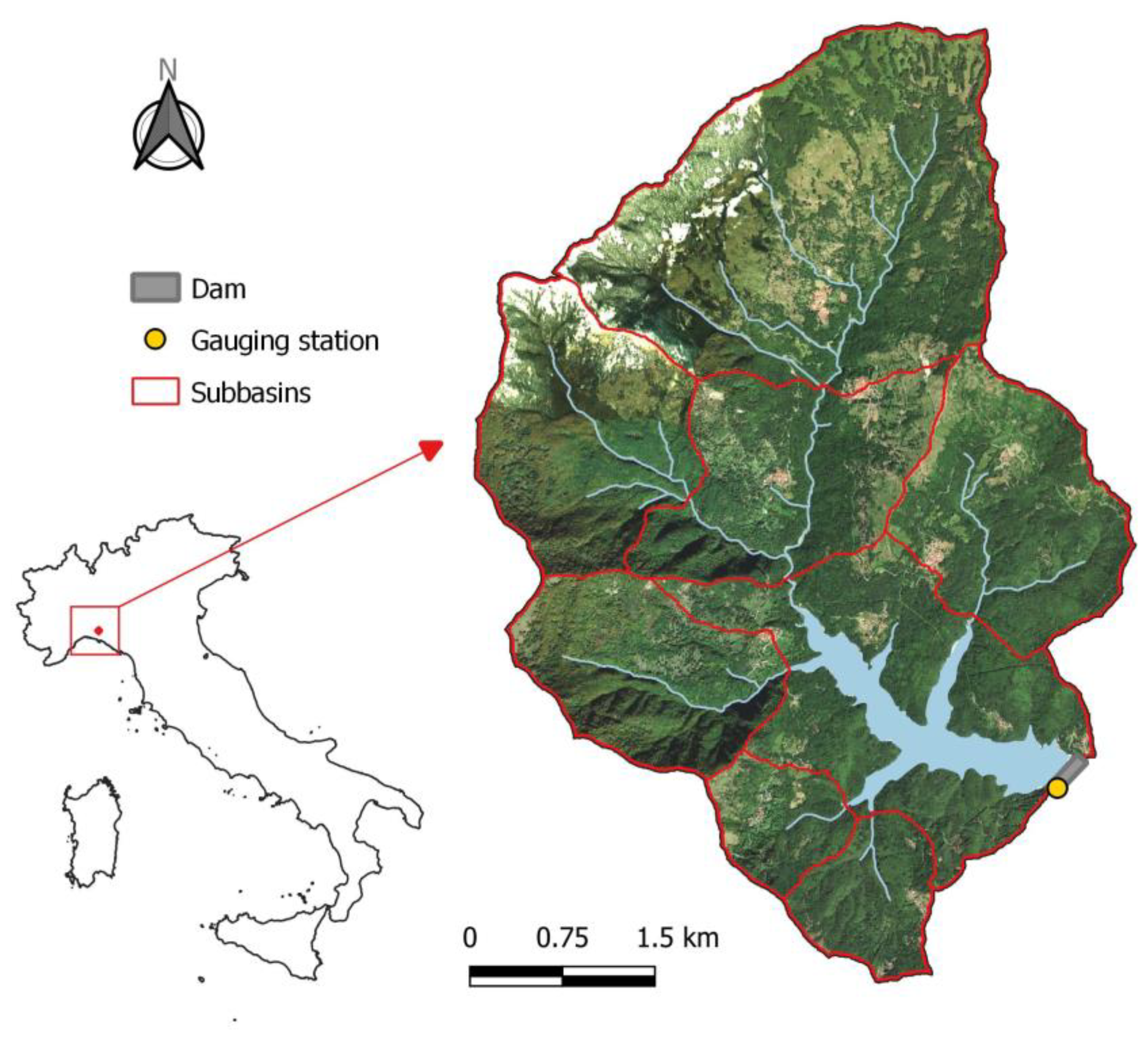
2.1. Study Area

The study area is a small catchment (26 km²) located upstream of Brugneto Dam, a concrete gravity structure on Brugneto River, a tributary of Trebbia River, in the Province of Genoa (Liguria Region, northern Italy).

The dam was built between 1956 and 1960 by the Municipalized Gas and Water Company (AMGA) of Genoa. It is 77.5 m high, and the dam crest is situated at an elevation of 780 m a.s.l. The catchment area extends up to 1597 m a.s.l. on Mount Antola, where the Brugneto River originates. The primary function of the dam is to support the provision of drinking water to the Province of Genoa. The reservoir behind the dam is referred to as Brugneto Lake, which has a capacity of approximately 25 million m³. The lake extends for a length of 3 km, with a maximum width of about 200 m. At the spillway crest level (777 m a.s.l.), the lake covers approximately 0.97 km². Due to the morphological configuration of the catchment, the lake exhibits several branches that gather runoff from different valleys (Figure 1). The main river that feeds into the lake (Brugneto River) has a length of about 5 km.

The predominant soil types consist mainly of clay loam and silty clay loam classes, as classified by the United States Department of Agriculture (USDA) soil classification system [33]. The data were retrieved from the geoportal of the Liguria Region: https://geoportal.regione.liguria.it/, accessed on 10 October 2023. The primary land cover in the Brugneto catchment consists of forested areas, covering nearly 72% of the total area, with an additional 23% covered by grassed areas. The remaining portion of the study area is divided between water bodies (4%) and urban districts (1%).

A shallow aquifer, which closely resembles the surface catchment, is present in the region. This aquifer is bounded at the base by rock formations, characterized by lithological variations and chaotic complexes, which hinder the recharge of deeper aquifers. As a result, most precipitation over the basin is discharged as shallow subsurface flow, with negligible outflows from the system.

2.2. Climate Data

2.2.1. Historical Data

The climate data used in this study included daily precipitation and mean temperature values recorded at a meteorological station located near the dam (Brugneto Dam gauging station, Figure 1). These data are freely available in the Dext3r service (https://simc.arpae.it/dext3r/, accessed on 10 October 2023) and “Hydrological Annals—Part I” (https://www.arpae.it/it/temi-ambientali/meteo/report-meteo/annali-idrologici/, accessed on 10 October 2023), provided by the Environmental Agency of the Emilia-Romagna Region (ARPAE). Precipitation data refer to the periods 1976–2005 and 2015–2020, while temperature data cover the period from 1976 to 2020. The gaps in the data series were filled by utilizing information from the closest monitoring stations, following the FAO method [34,35].

The meteorological data for the period from 1976 to 2005, assumed as the control period, were utilized to analyze historical climate and adjust the bias in the climate model data used for future projections. The data collected over the remaining periods were used as the input for hydrological model calibration and validation. Temperature data were employed to calculate potential evapotranspiration through the Thornthwaite method [36].

The historical climate was investigated by calculating precipitation and temperature regimes and trend analyses on a monthly scale. The Mann–Kendall test [37,38] was used to detect the presence of monotonic trends in the time series at a 5% significance level. The Mann–Kendall test is a statistical non-parametric test; thus, it is not affected by assumptions about the underlying distribution of the data. This test identifies potential trends by comparing the number of concordant and discordant pairs of data points. In particular, it recognizes the presence of a trend if the number of concordant pairs significantly exceeds the number of discordant pairs or vice versa. Since the Mann–Kendall test assumes data independence, the correction recommended by Hamed and Rao [39] was applied to account for data serial correlation. The non-parametric Theil–Sen statistical estimator [40] was used to quantify the magnitude of the identified trend. In the Theil–Sen method, the trend slope is determined as the median of the slopes computed for all possible pairs of data points. Unlike parametric approaches (such as least square linear regressions), the Theil–Sen method is particularly robust in the presence of outliers, thereby providing a reliable measure of the trend without being influenced by extreme values.

2.2.2. Future Climate Projections

This study exploits the daily precipitation and temperature projections of the EURO-CORDEX initiative [32], which can be freely accessed at https://www.euro-cordex.net/ (accessed on 10 October 2023). An ensemble of 13 combinations of General Circulation Models (GCMs) and Regional Climate Models (RCMs) was considered (

Table 1. Climate models (GCM-RCM combinations) from the EURO-CORDEX initiative used in this study. The ditto mark “ indicates repetition of the above text.

	GCM	RCM
1	CNRM-CM5	CCLM4-8-17
2	“	RCA4
3	“	RACMO22E
4	EC-EARTH	RACMO22E
5	“	RCA4
6	“	CCLM4-8-17
7	“	HIRHAM5
8	IPSL-CM5A-MR	WRF381P
9	“	RCA4
10	“	WRF331F
11	MPI-ESM-LR	CCLM4-8-17
12	“	RCA4
13	NorESM1-M	HIRHAM5

).

Each climate model includes a historical simulation, spanning from 1950/1970 to 2005, and scenario simulations based on different Representative Concentration Pathways (RCPs) for the period from 2006 to 2100. In this work, the RCP4.5 and RCP8.5 scenarios were considered. RCP4.5 is an intermediate scenario that assumes moderate greenhouse gas emissions and efforts to mitigate climate change. In contrast, RCP8.5 is a high-emission scenario in which greenhouse gas emissions continue to increase throughout the 21st century without significant mitigation efforts. The EURO-CORDEX models provide data on a regular grid with a resolution of approximately 12.5 km (EUR-11 grid). The model outputs were downscaled at the meteorological station location (Brugneto Dam gauging station) through an inverse distance interpolation method with a power of two. The RCM data regarding the nine grid cells closest to the selected station were interpolated to obtain site-specific time series.

Climate model projections often exhibit systematic deviations from the observed climate. To enhance the reliability of these projections, especially for hydrological impact assessments, a bias correction is essential [11]. To this end, the distribution mapping method [13,41,42,43] was adopted in this study. Through this method, the cumulative distribution functions of the climate model data were aligned with those of the observed data during the control period (1976–2005) for each month. The Gaussian distribution function was used to model temperature data, and the Gamma distribution function was used to model wet day rainfall. Before applying the distribution mapping method, the number of rainy days in the climate models was adjusted by identifying suitable thresholds for each model, so that the modeled number of rainy days matched the observed one during the control period. All projected precipitation values below this threshold were set to zero. The same transfer functions and thresholds, calculated for each month and each model during the control period, were then used to correct projected temperature and precipitation data throughout the scenario simulations. The bias-corrected temperature data were used to compute the future potential evapotranspiration.

2.3. Hydrological Data

Since several river branches gather flow directly into the lake, measures of the inflow discharge into Brugneto Lake are not available. Daily measurements of the lake water level from January 2015 to December 2020 are available, as well as records of the discharged volume from the dam. This outflow volume includes that used for drinking water, the volume supplied to the land reclamation authority for irrigation use, the ecological flow, and the overflow volume. Furthermore, the relationship between storage and water level elevation (i.e., the reservoir volume–elevation curve), obtained through a topographical survey, exists.

Under the level pool approximation, the continuity equation establishes a connection between the difference in inflow and outflow from the reservoir and the rate of change in the reservoir’s storage [44]. Accordingly, the continuity equation was solved to estimate the unknown inflow through the reverse level pool routing method [44,45]. Negative inflow values can be calculated using this method, even following the recommendations by Zoppou [44], due to measurement errors. To overcome this problem, a zero-inflow discharge was assigned whenever the calculated value turned negative.

Figure 2 shows the estimated inflow to the lake for the period from 2015 to 2020, along with the recorded outflow and lake water levels. The same figure also includes the reservoir volume–elevation curve.

2.4. Hydrological Modeling

2.4.1. The Hydrologic Modeling System (HEC-HMS)

In this study, we used the Hydrologic Engineering Center’s Hydrologic Modeling System (HEC-HMS, version 4.9) [46] to simulate the hydrological processes occurring within the watershed considered.

The HEC-HMS is a freely available software developed by the U.S. Army Corps of Engineers. It is a physically based and conceptually semi-distributed model, extensively described in various literature sources (e.g., [28,46,47,48]). It allows for dividing the watershed into several subbasins, each with its own specific characteristics.

The HEC-HMS can be employed as either an event-based or continuous rainfall–runoff model. Given our focus on future water resources, we opted for a continuous simulation, including the temporal changes in soil storage and evapotranspiration. For continuous simulations, we employed the soil moisture accounting (SMA) model [46] to replicate water losses during both dry and wet periods. The SMA model, in combination with canopy and surface methods, simulates the movement and storage of water for each subbasin, encompassing the land surface, soil profile, and multiple groundwater layers [49].

The SMA model conceptualizes the watershed with a series of storage layers [47,50,51]: (I) canopy-interception storage, where precipitation intercepted by the canopy is stored, does not reach the soil surface, and is removed only by evaporation; (II) surface-interception storage, where precipitation not captured by canopy interception can be stored on the surface and may infiltrate or become surface runoff; (III) soil-profile storage, where infiltrated water can be stored in the top soil layer, and water from this storage can either percolate to a groundwater layer or be eliminated through evapotranspiration; and (IV) groundwater storage (comprising up to two layers), representing horizontal interflow processes. Losses from a groundwater storage layer occur due to groundwater flow (baseflow) or percolation between layers (note that aquifer flow is not explicitly modeled). The linear reservoir method was used to represent the baseflow contribution to the outflow from the subbasins. Precipitation and evapotranspiration time series data are essential meteorological inputs for the simulation, which were detailed at a daily scale.

The Clark Unit Hydrograph method was used to compute surface runoff. Specifically, the standard version of the method, in which the time of concentration and the storage coefficient parameters do not depend on the intensity of excess precipitation, was applied. The kinematic wave model was used to simulate the flood routing within the river network [46], assuming a rectangular channel for simplicity.

The HEC-HMS requires specifying the value of various parameters governing the relationship between system input and output.

Table 2. Subbasin and reach parameters appearing in the HEC-HMS. Criteria used to make an initial estimation of the parameters. Parameters involved in the calibration process are indicated with the symbol *.

Parameter	Units	Initial Estimate Criteria	Module
Maximum canopy storage	mm	Land cover [50,52]	Soil Moisture Accounting (SMA)
Maximum surface storage	mm	Land cover [50,52]
Maximum infiltration rate *	mm/h	Soil type [53]
Impervious surface area	%	Land cover
Total soil storage *	mm	Soil type [54,55]
Soil tension storage *	mm	Soil type [54,55]
Soil percolation *	mm/h	Soil type (hydraulic conductivity) [49,55]
Groundwater1 * and 2 * storage	mm	Flow–recession curves [49]
Groundwater 1 * and 2 percolation	mm/h	Soil type (hydraulic conductivity) [49,55]
Groundwater 1 * and 2 * coefficient	h	Flow–recession curves [49]
Groundwater 1 and 2 fraction	-	Not needed using SMA	Baseflow—linear reservoir
Groundwater 1 and 2 storage coefficient	h	12 h, the minimum for daily-scale simulations [46]
Time of concentration	h	Kirpich formulation [56]	Clark unit hydrograph
Storage coefficient	h	Time of concentration and land cover [57]
Length	m	DEM	Kinematic wave
Slope	m/m	DEM
Manning’s coefficient	s/m1/3	River bed material [58]
Width	m	DEM

provides a list of these parameters for each subbasin and river reach.

2.4.2. Model Setup

The delineation of the basin upstream of the dam and relative subbasins was accomplished by utilizing an available digital terrain model (DEM) of the study area with a spatial resolution of 5 m, combined with the GIS tools integrated into the HEC-HMS. Given the relatively small size of the catchment, one subbasin was identified for each of the river branches which flow into the lake. An exception was made for the northernmost branch (the main one), whose subbasin was subdivided into three smaller subbasins (Figure 1).

In the modeling process, only the main reach was considered for flood propagation, neglecting the other reaches due to their relatively short lengths.

Several model parameters must be set before simulations (Table 2). Initial values for these parameters were established based on the geological features, soil type, and land cover characteristics of the area, as well as on expert knowledge. Table 2 outlines the criteria used to make an initial estimation of these parameters, along with the pertinent literature references to assist in their initialization.

Furthermore, precipitation and potential evapotranspiration (ETP) time series are essential for continuous simulations. These data were provided on a daily scale, as data concerning shorter time windows were not available. To obtain daily ETP values, the monthly ETP, evaluated with the Thornthwaite formula, was equally distributed for each day of the corresponding month. Evapotranspiration was enabled in both dry and wet periods.

The final values of the parameters were estimated through calibration.

2.4.3. Model Calibration

The calibration and validation of the hydrologic model were performed on the basis of the total inflow to the lake, using the data referring to the period from 2015 to 2020. In particular, the year 2015 was employed as a warm-up period to compensate for inaccuracies in defining the initial conditions, the period from 2016 to 2019 was dedicated to calibration, and the year 2020 was used for validation.

The PEST (Parameter Estimation) software package v. 17 [59] was employed to automatically calibrate the HEC-HMS model through minimization of the weighted sum of square differences between observed data and simulated results. An iterative process, which requires the computation of derivatives of model outputs with respect to the parameters to be estimated, was used to handle the non-linear parameter estimation. PEST calculates these derivatives using finite differences.

Sensitivity analysis of the model outputs to the model parameters shows that some parameters are irrelevant and could be excluded from the calibration, retaining their initially estimated values. Table 2 indicates the parameters considered in the automatic calibration process with asterisks.

To speed up the calibration process, the adjustable parameters were not individually estimated for each subbasin. Instead, parameters of the same type were tied together for all subbasins. Accordingly, PEST adjusted these parameters simultaneously, preserving their initial ratios. This strategy maintains heterogeneity among subbasins without overly burdening the calibration process.

Figure 3 compares observed and estimated discharge after the calibration process. On the whole, the model satisfactorily replicates the observed values, although some data points in the calibration set (2016–2019) exhibited significant deviations from the 1:1 line, especially for the highest observed flow values. This discrepancy could be explained by the use of daily rainfall data, which may not fully capture the formation of the most significant flood events in small basins. However, it is worth noting that this article focuses on water resource availability, rather than providing an in-depth description of flood events. The coefficient of determination from the linear regression for the calibration period has a satisfactory value (R² = 0.74). Furthermore, in the validation period (year 2020), data points exhibited a smaller deviation from the 1:1 line.

To globally evaluate the discrepancy between simulated and observed discharges for both the calibration and validation periods, three different metrics were employed: (1) the Volume Bias, which represents the ratio of the difference in observed and simulated volumes to the observed volume; (2) the Nash–Sutcliffe efficiency, which evaluates the model’s ability to replicate the shape of discharge time series with values ranging from 0 to 1, and 1 indicating the best performance; and (3) the Root Mean Square Error (RMSE), which quantifies the discrepancy between observed and simulated discharges.

Table 3. Model performance metrics for the calibration and validation periods.

Metrics	Calibration Period	Validation Period
Volume Bias	−0.21%	5.68%
Nash–Sutcliffe	0.733	0.607
RMSE	17.31	11.04

reports the values of these metrics for both the calibration and validation periods. The model performance is generally good within the calibration period, but is slightly worse in terms of bias and Nash–Sutcliffe values within the validation period. The RMSE shows a slightly lower value during the validation period. The overall performance of the model is satisfactory, demonstrating that the model is able to effectively capture the most significant hydrological aspects.

3. Results

3.1. Climate Analysis

3.1.1. Historical Climate

Table 4. Precipitation and temperature monthly mean values and Sen slopes (Trend), evaluated during the period from 1976 to 2005 at Brugneto Dam gauging station. The symbol * indicates a significant trend at the 5% level.

	Precipitation		Temperature
	Mean (mm)	Trend (mm/decade)	Mean (°C)	Trend (°C/decade)
Jan	157.1	−1.5	1.48	+0.39
Feb	91.7	−11.2	1.91	+0.29
Mar	130.4	−28.7	4.63	+0.67
Apr	161.1	+9.6	7.02	+0.64 *
May	135.8	+3.1	11.48	+1.07 *
Jun	98.9	−6.2	15.54	+0.76 *
Jul	69.7	+8.2	17.98	+0.29
Aug	92.8	−9.7	17.85	+0.85 *
Sep	165.6	+10.2	13.92	+0.41
Oct	285.9	−9.3	10.30	+0.61 *
Nov	225.0	+44.6	5.48	+0.60 *
Dec	196.0	−7.8	2.62	+0.23
Year	1810.1	+73.4	9.18	+0.63 *

provides monthly and annual historical climate analysis data for the Brugneto Dam meteorological station over the period from 1976 to 2005. The average annual precipitation was approximately 1810 mm, but the rainfall distribution throughout the year was not evenly spread. The month of October recorded the highest precipitation, with an average monthly value of approximately 286 mm, whereas July was the driest month, with 70 mm of precipitation on average. The precipitation trend varied by month, with some months experiencing decreasing trends and others increasing trends. November showed the most significant increase in precipitation (44.6 mm/decade), while March had the most significant decrease (−28.7 mm/decade). However, the precipitation trend was never statistically significant within the period considered.

Temperature data indicated well-defined seasonal variations. The annual average temperature for the 30-year period, from 1976 to 2005, was about 9.2 °C, with January being the coldest month (1.5 °C on average) and July the warmest (18 °C on average). The temperature trend also varied by month, but it systematically showed positive values, denoting continuous warming within the period considered. In several months, the trends were statistically significant at the 5% level. May had the most significant warming trend, of 1.07 °C per decade; the annual temperature exhibited a significant upward trend of 0.63 °C per decade.

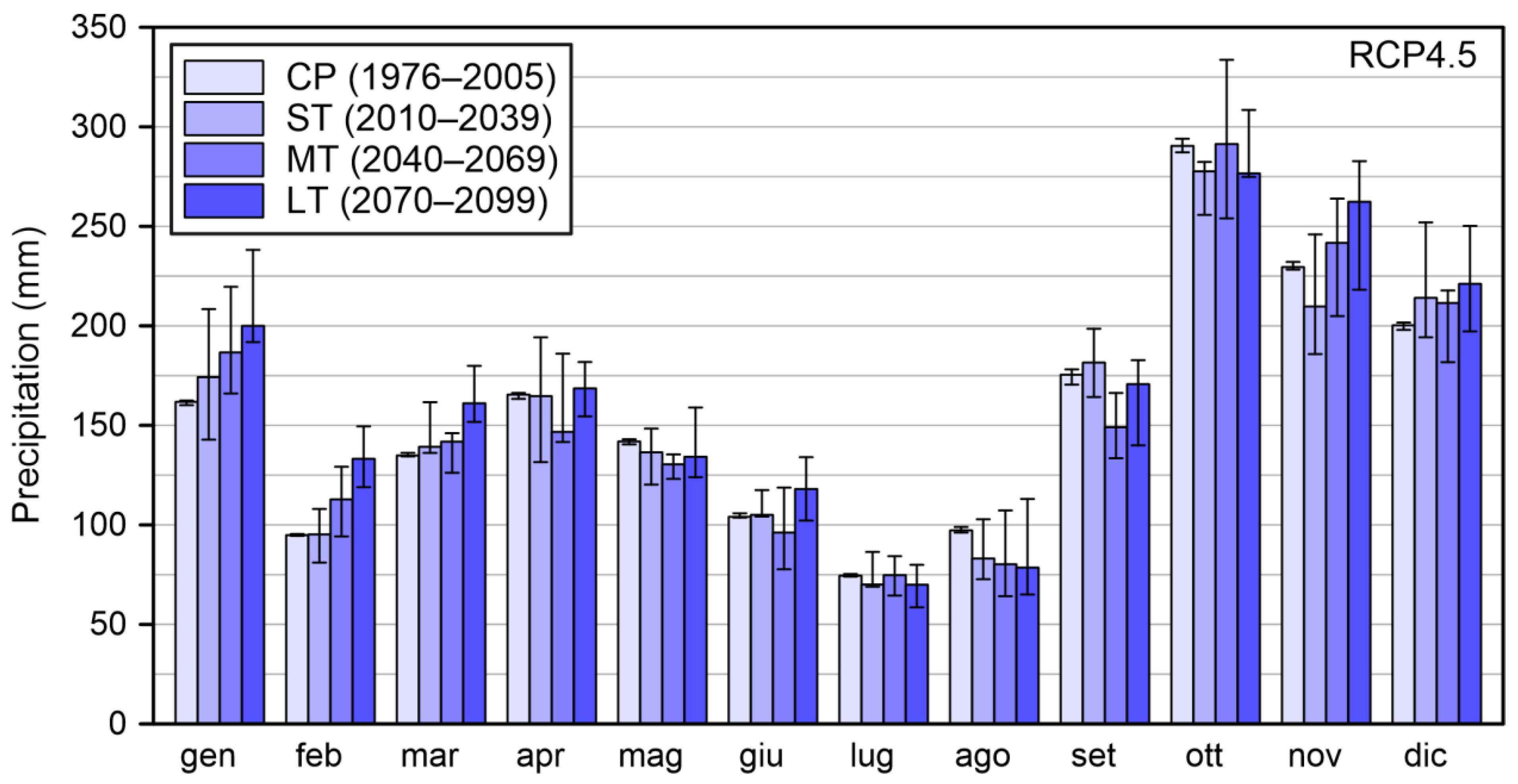
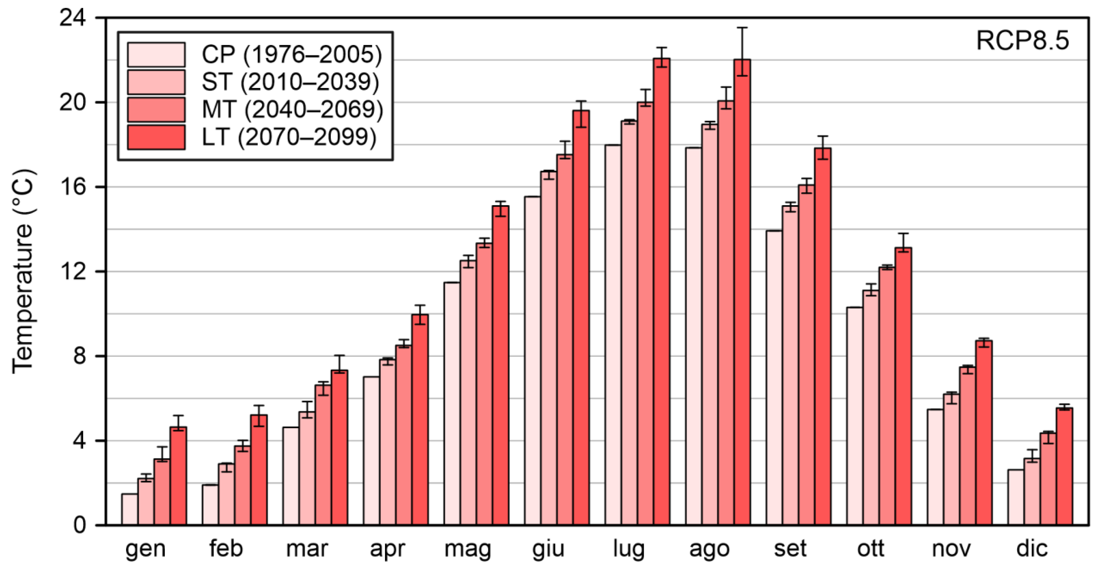
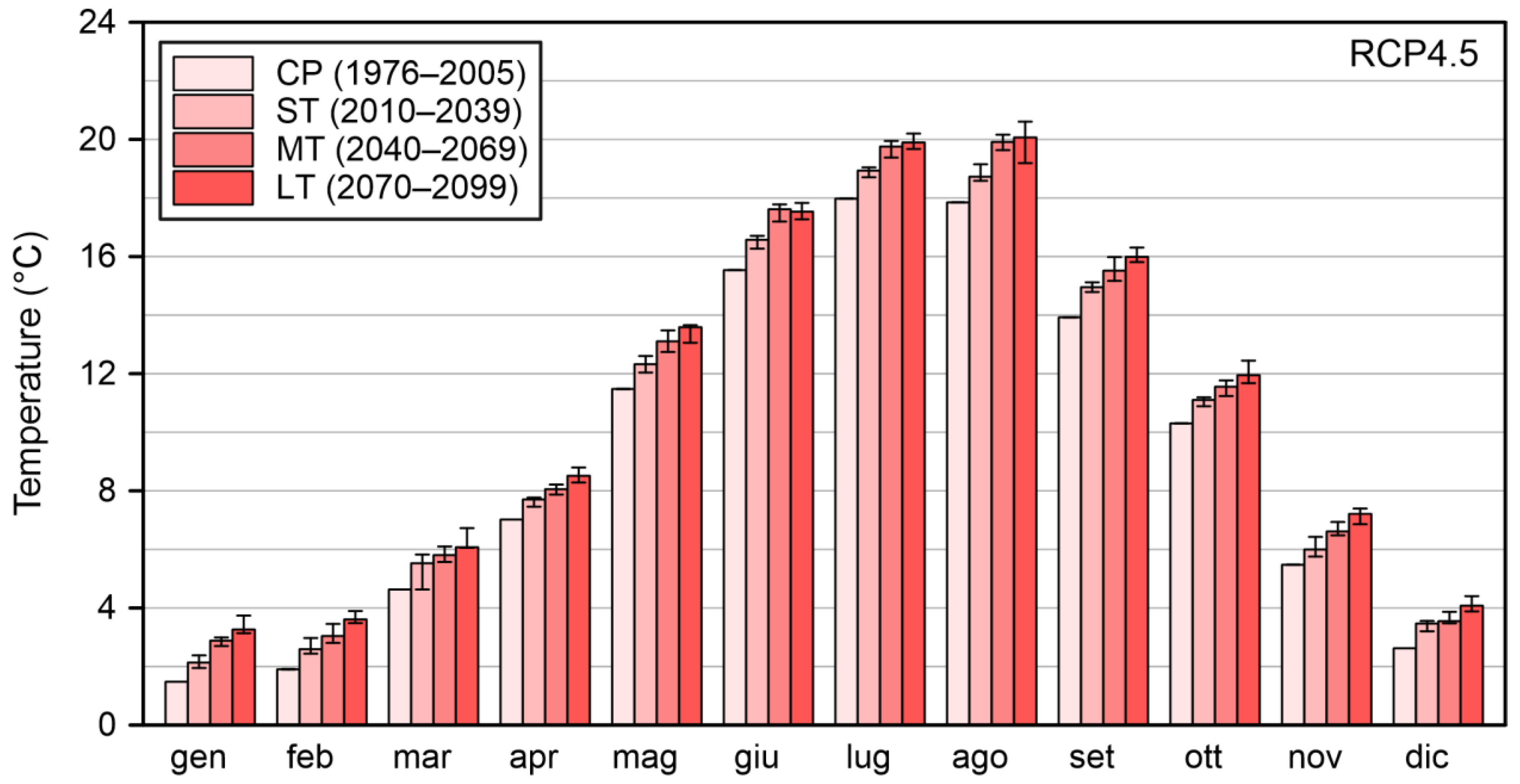
3.1.2. Future Climate Projections

Bias-corrected data from 13 RCMs were used to investigate future climate conditions in the study area. The climate variables were analyzed over four 30-year periods that included a control period (CP) from 1976 to 2005, followed by three future periods: 2010–2039 (short-term, ST), 2040–2069 (medium-term, MT), and 2070–2099 (long-term, LT). The analysis focused on monthly and annual precipitation, as well as monthly and annual mean temperature, considering two emission scenarios: RCP4.5 and RCP8.5.

Figure 4 and Figure 5 present the results for precipitation under the RCP4.5 and RCP8.5 scenarios, respectively. For each month, the precipitation projected at different time intervals is displayed in terms of RCM medians, along with climate model uncertainty represented by the RCM interquartile range.

Table 5. RCM median values of monthly precipitation (in mm) during the control period (CP, 1976–2005), and precipitation changes (%) among the RCM medians at the short- (ST, 2010–2039), medium- (MT, 2040–2069), and long-term (LT, 2070–2099) periods, compared to those obtained during the control period, for the RCP4.5 and RCP8.5 scenarios.

		RCP4.5			RCP8.5
	CP	ST	MT	LT	ST	MT	LT
Jan	161.9	+7.6%	+15.3%	+23.6%	+2.1%	+24.0%	+16.2%
Feb	94.9	+0.3%	+18.9%	+40.3%	+11.6%	+20.2%	+14.0%
Mar	134.9	+3.2%	+5.1%	+19.4%	+3.3%	+13.4%	+16.5%
Apr	165.5	−0.5%	−11.3%	+1.9%	−8.8%	−2.8%	−12.6%
May	141.9	−3.8%	−8.1%	−5.4%	+2.7%	−0.6%	−16.7%
Jun	104.1	+0.9%	−7.6%	+13.4%	−4.0%	+3.3%	−13.1%
Jul	74.5	−5.9%	+0.4%	−6.1%	+2.0%	−5.2%	−27.7%
Aug	97.2	−14.5%	−17.5%	−19.2%	−13.7%	−14.4%	+15.8%
Sep	175.5	+3.5%	−15.1%	−2.7%	−4.9%	−14.3%	−19.3%
Oct	290.4	−4.4%	+0.3%	−4.8%	−14.4%	+0.5%	−17.4%
Nov	229.5	−8.6%	+5.3%	+14.3%	+5.9%	+8.8%	+9.5%
Dec	200.3	+6.9%	+5.6%	+10.4%	−1.5%	+2.9%	+12.9%
Year	1872.3	+3.1%	+2.0%	+8.4%	+1.7%	+4.9%	−3.0%

summarizes monthly and annual precipitation values (RCM median) evaluated within the CP, as well as the percentage changes expected in the ST, MT and LT, compared to the control period, for the RCP4.5 and RCP8.5 scenarios. The outcomes vary across different months. The RCP4.5 scenario shows a significant increase in precipitation from November to March, except for a short-term decrease in November (−8.6%). The highest increase occurs in February (+40.3%, LT). The months from April to October present a prevalent precipitation decrease, apart from an increase in the LT in June (+13.4%) and some other slight positive changes of less than 3.5%. In particular, August exhibits a progressive decrease in precipitation (−19.2% in the LT). The annual precipitation for the future periods is generally higher than during the control period, with small variations in the ST and MT and an increase of 8.4% in the LT.

According to the RCP8.5 scenario, the precipitation is projected to increase from November to March for all considered time periods, except for in the ST in December. The highest decrease is estimated for January (+24%, MT). Precipitation is projected to decrease during the months from April to October, with some minor positive changes of less than 3.3% and a notable increase in the LT in August (+15.8%). July experiences the most severe reduction in precipitation (−27.7%, LT). Annual precipitation variations across the three future periods are less than 5%, with small decreases in the ST and MT and an increase in the LT.

It is worth noting that there is considerable variability among the 13 RCMs, as indicated by the spread between the 25th and 75th percentiles (Figure 4 and Figure 5). This variability highlights the complexity of precipitation climate projections and the need to assess model uncertainty.

Figure 6 and Figure 7 show projected changes in monthly average temperatures across the four periods considered based on the RCP4.5 and RCP8.5 scenarios, respectively.

Table 6. RCM median values of monthly mean temperature (in °C) during the control period (CP, 1976–2005), and differences among the RCM medians at the short- (ST, 2010–2039), medium- (MT, 2040–2069), and long-term (LT, 2070–2099) periods, as well as those obtained during the control period for the RCP4.5 and RCP8.5 scenarios.

		RCP4.5			RCP8.5
	CP	ST	MT	LT	ST	MT	LT
Jan	1.48	+0.66	+1.41	+1.78	+0.73	+1.65	+3.17
Feb	1.91	+0.69	+1.13	+1.70	+0.99	+1.84	+3.31
Mar	4.63	+0.90	+1.17	+1.44	+0.73	+1.99	+2.70
Apr	7.02	+0.69	+1.04	+1.50	+0.81	+1.49	+2.94
May	11.48	+0.85	+1.62	+2.11	+1.04	+1.86	+3.63
Jun	15.54	+1.03	+2.08	+2.00	+1.19	+1.99	+4.07
Jul	17.98	+0.96	+1.78	+1.92	+1.13	+2.03	+4.10
Aug	17.85	+0.88	+2.07	+2.22	+1.11	+2.22	+4.17
Sep	13.92	+1.03	+1.60	+2.07	+1.18	+2.17	+3.91
Oct	10.30	+0.80	+1.25	+1.65	+0.80	+1.89	+2.82
Nov	5.48	+0.52	+1.13	+1.74	+0.72	+2.00	+3.25
Dec	2.62	+0.85	+0.93	+1.45	+0.54	+1.74	+2.92
Year	9.18	+0.80	+1.43	+1.79	+0.96	+1.83	+3.32

summarizes these results in terms of RCM median differences among the future periods and the control period at monthly and annual scales.

The analysis shows a progressive warming across all months for both emission scenarios. According to RCP4.5, the mean temperature is expected to increase, from a maximum of 0.9 °C in the ST up to 1.8 °C in the LT, from October to April. The months from May to September experience significant temperature increases, from about 1.0 °C in the ST up to more than 2 °C in the LT. The annual mean temperature increases from 0.8 °C (ST) up to 1.8 °C (LT). The warming rate is even more severe under the RCP8.5 scenario. The months from October to April show a temperature increase of about 1.0 °C in the ST up to about 3 °C in the LT. Temperature increases from about 1 °C in the ST up to more than 4 °C in the LT are expected from May to September. The annual mean temperature increases from 1 °C (ST) up to 3 °C (LT). The inter-model variability (Figure 6 and Figure 7) is quite limited, and lower than that assessed for precipitation, denoting that all of the climate models considered agree with the warming trend.

3.2. Hydrological Analysis

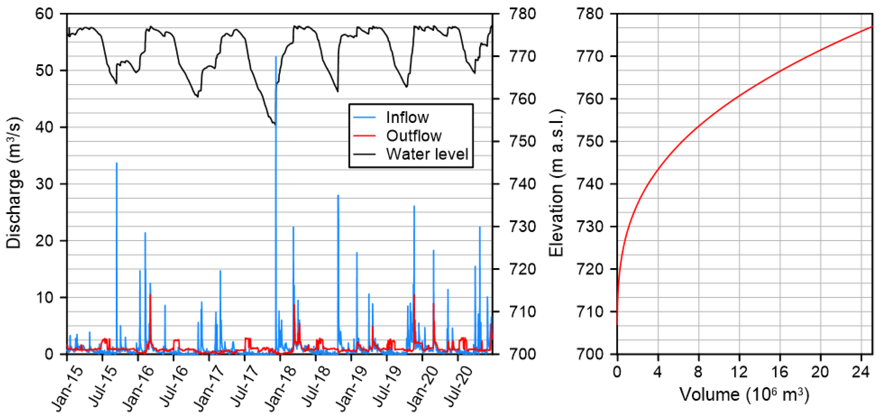
3.2.1. Historical Period

The calibrated hydrological model was used to determine the inflow to Brugneto Lake for the historical period from 1976 to 2005.

Table 7. Monthly and annual averaged inflow (in m³/s) to Brugneto Lake during the period from 1976 to 2005.

Jan	Feb	Mar	Apr	May	Jun	Jul	Aug	Sep	Oct	Nov	Dec	Year
1.52	1.02	0.97	1.16	0.74	0.35	0.14	0.05	0.43	1.63	1.87	1.61	0.96

reports the monthly and annual inflow discharges averaged over the control period.

The flow regime is pluvial, with liquid precipitation predominating across all seasons. This leads to a strong correlation between precipitation and flow discharge. The flow regime exhibits significant interannual variability. The highest discharge values occurred during the autumn and winter months, with a maximum in November, with an average discharge value of approximately 1.9 m³/s. The lowest values were observed during the summer months, with an absolute minimum of approximately 0.05 m³/s in August.

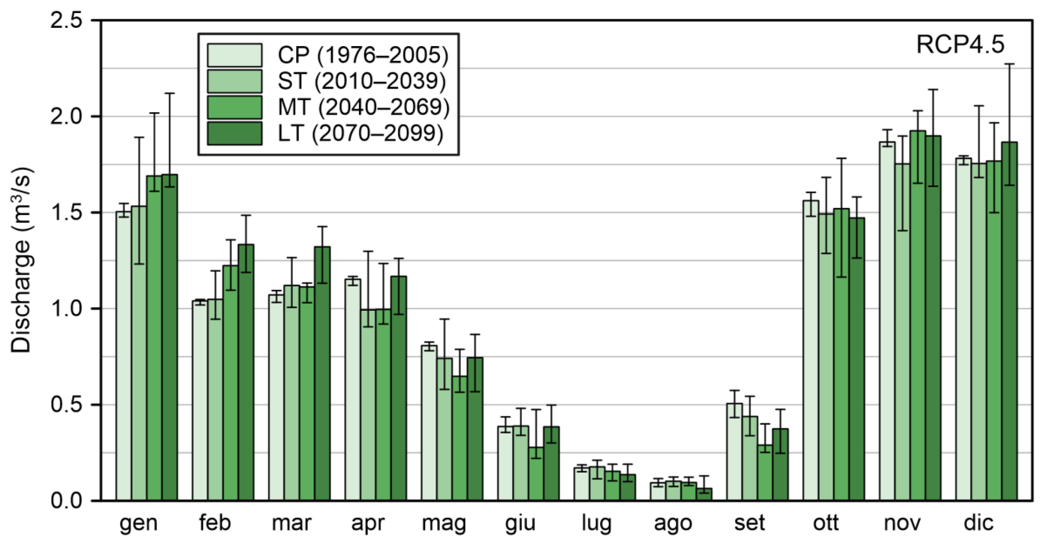
3.2.2. Future Scenarios

The future inflow to Brugneto Lake was assessed for the same periods as for the meteorological variables. Figure 8 and Figure 9 show the monthly average inflow discharges projected under the RCP4.5 and RCP8.5 scenarios, respectively.

Table 8. RCM median values of monthly averaged inflow discharge during the control period (CP, 1976–2005), and changes (%) among the RCM medians at the short- (ST, 2010–2039), medium- (MT, 2040–2069), and long-term (LT, 2070–2099) periods, compared to those obtained during the control period, for the RCP4.5 and RCP8.5 scenarios.

		RCP4.5			RCP8.5
	CP	ST	MT	LT	ST	MT	LT
Jan	1.50	+1.9%	+12.4%	+12.8%	−1.0%	+11.7%	+4.6%
Feb	1.04	+0.8%	+17.6%	+28.2%	+3.5%	+11.7%	+14.2%
Mar	1.07	+4.6%	+3.9%	+23.4%	+4.0%	+5.4%	+11.6%
Apr	1.15	−13.9%	−13.6%	+1.3%	−15.7%	−3.7%	−23.0%
May	0.81	−8.2%	−19.8%	−7.8%	−3.1%	−11.5%	−32.6%
Jun	0.39	+0.7%	−28.0%	−0.3%	+5.2%	+2.8%	−44.1%
Jul	0.17	+3.0%	−10.2%	−20.5%	−7.8%	−21.2%	−66.4%
Aug	0.09	+9.1%	+1.4%	−31.3%	+6.2%	−25.4%	−21.1%
Sep	0.51	−13.4%	−42.7%	−26.1%	−24.7%	−36.7%	−40.1%
Oct	1.56	−4.4%	−2.7%	−5.7%	−28.4%	−10.2%	−32.0%
Nov	1.87	−6.1%	+3.1%	+1.7%	+1.2%	+1.6%	−4.5%
Dec	1.78	−1.6%	−0.8%	+4.7%	−5.7%	−0.5%	−0.9%
Year	1.00	+3.0%	−0.6%	+7.4%	−2.4%	+3.0%	−6.0%

summarizes the results, presenting the differences in RCM medians among the future periods and the control period on both monthly and annual scales.

The variations in discharge are generally consistent with those in precipitation. The monthly discharge values for the RCP4.5 scenario exhibit increases during the months from January to March, with the highest increase expected for February (+28.2%, LT). The period spanning April through October denotes a prevalent discharge decrease, except for an increase in the ST in August (+9.1%), as well as some other minor positive changes of less than 3%. However, it is noteworthy that the percentage changes for July and August are calculated with reference to very small values. The months of November and December present slight positive and negative variations. In terms of annual values, the discharge increases by 3% in the ST, stays nearly stable in the MT, and reduces by 7.4% in the LT. According to the RCP8.5 scenario, the inflow discharge will increase in the months from January to March, even if the variations are projected to be less pronounced than those estimated under the RCP4.5 scenario. Also, in this case, the highest increase is estimated for the month of February (+14.2%, LT). Discharges are expected to experience a reduction from April to October, with some exceptions for slight increases in June in the ST and MT and August in the ST. July shows the most severe discharge decrease (−66.4%, LT). The months of November and December present discharge variations of less than 6%. As regards the annual values, the water resource slightly decreases in the ST (−2.4%) and LT (−6%), and increases in the MT (+3%).

Figure 10 shows the flow–duration curves (FDCs) obtained considering the daily discharges of the single RCMs and the whole RCM ensemble for the three future periods and both emission pathways, RCP4.5 and RCP8.5. FDCs are valuable for understanding how water availability may be altered, since they provide a comprehensive view of the range of river discharges. For comparison, the FDCs obtained in the CP are also included in Figure 10. In addition,

Table 9. Discharges (in m³/s) corresponding to ¼ 365 days (Q_wet), ½ 365 days (Q_mid), and ¾ 365 days (Q_dry), evaluated using the entire RCM ensemble during the control period (CP, 1976–2005), and in the short- (ST, 2010–2039), medium- (MT, 2040–2069), and long-term (LT, 2070–2099) periods under the RCP4.5 and RCP8.5 scenarios.

		RCP4.5			RCP8.5
	CP	ST	MT	LT	ST	MT	LT
Qwet	1.01	0.96	0.96	0.98	0.95	0.97	0.83
Qmid	0.37	0.34	0.32	0.33	0.32	0.33	0.26
Qdry	0.10	0.09	0.07	0.08	0.08	0.08	0.06

provides an overview of the flow rates predicted for selected durations. Specifically, the flow discharges corresponding to ¼ 365, ½ 365, and ¾ 365 days were reported to represent wet, median, and dry hydrological conditions, respectively. Referring to the ST period and the entire ensemble of RCMs, a slight reduction in inflow is estimated, compared to the CP, for both the RCP4.5 and RCP8.5 scenarios. This reduction is more evident for low discharges. The curves obtained from individual RCMs show a higher degree of variability for the RCP4.5 scenario in comparison with the RCP8.5 one. Similar considerations can be made for the MT, although a more pronounced decline in low flow rate values is expected. Inter-model variability also increases, especially for the RCP8.5 scenario. In the LT, the results under the RCP4.5 scenario are similar to those of the previous period when considering the whole RCM ensemble. Under the RCP8.5 scenario, a more pronounced downward shift in future FDCs can be expected, although an increase in high flows is highlighted for very short durations. The model variability increases, but the majority of CDFs fall below those of the CP, denoting an expected future decrease in the available water resource.

4. Discussion and Conclusions

This study aimed to assist and enhance future water management for the Brugneto Dam by investigating how climate change will affect water availability. To this end, the future inflow to Brugneto Lake was estimated through a combination of climate change scenarios and hydrological modeling.

The first significant aspect to discuss pertains to the uncertainty of the study findings. To account for uncertainty in climate scenarios, an ensemble of climate model projections and two distinct emission pathways were examined. For precipitation, the inter-model variability exceeded the median changes across the short-, medium-, and long-term periods for both scenarios. This indicated a substantial level of uncertainty in projecting precipitation. Conversely, temperature data displayed less uncertainty, with the climate models generally in agreement regarding temperature increases in the study area. This uncertainty extended into the hydrological modeling phase, leading to uncertainties in simulated river discharges. In many cases, variations among different models exceeded the median variations among future time periods, indicating a high degree of uncertainty for river discharges, as well. These findings are in accordance with those of Versini et al. [24] for Llobregat River Basin in Spain. Furthermore, additional factors, such as uncertainty in hydrological model parameters and the hydrological model itself, should also be taken into account. Additionally, downscaling and bias-correction methods for the climate projections introduce further sources of uncertainty that can impact the final results. Handling a large ensemble of climate models, as executed in this study, can pose significant computational demand. It is worth noting that the authors of many studies in the literature opted to restrict the analysis to just one or a few climate models and scenarios. Given these circumstances, it also becomes challenging to consider multiple hydrological models (each requiring setup and calibration) and different downscaling/bias-correction methods. Consequently, the inclusion of all sources of uncertainty may become impractical, if not unfeasible. However, when the hydrological model is well-calibrated, the related uncertainty tends to become less significant [24], and the primary sources of overall uncertainty often are climate model projections. Comparative analyses with alternative hydrological models or different model setups may help to discern the impacts of the various sources of uncertainty. This aspect may be the subject of a future investigation.

Calibrating a semi-distributed (or even more so, a distributed) hydrological model involves various parameters, each of which typically differs for every subbasin. Nowadays, automatic calibration, using specific software, is generally preferred over manual calibration procedures [60]. Calibration necessitates observations that correspond to the simulated values, which, in the context of a hydrological model, typically refer to river discharges. Often, collecting a robust calibration dataset, both in terms of recorded period and location, is difficult, due to the limitations in the availability of gauging stations, especially in small basins. This situation was also encountered in the case study considered in this paper, in which the only feasible approach to obtaining useful inflow discharge data was by employing the reverse level pool routing method [45]. Consequently, in hydrological model calibration, it is common to deal with more parameters than can be uniquely constrained by the available observations, resulting in an ill-posed inverse problem. In such circumstances, a regularization approach is required to obtain a unique solution [61]. There are various regularization techniques available, including mathematical and manual methods [61,62]. A simple manual regularization technique entails using the same parameter values for all subbasins (lumped method) [62]; however, this can lead to excessive simplification. A more effective manual regularization approach involves estimating values for combinations of parameters, rather than individual parameters. As an example, these parameter combinations tie together the same parameters from different subbasins, causing them to vary in unison, while maintaining fixed ratios to one another [59]. This method, which was employed in this work, avoids oversimplification while guaranteeing computational efficiency. At the same time, it preserves the distinct characteristics and variations identified through the selection of different initial parameter values for each subbasin based on expert knowledge [28].

Another important aspect to acknowledge is the potential impact of changes in land cover and land use on future water resources. Land cover and use modifications, including urbanization, deforestation, and agricultural expansion, are well-established factors significantly affecting hydrological systems in various regions (e.g., [63,64,65]). However, this aspect has not been explicitly addressed within this paper. It is worth noting that the study area is situated within a mountainous region, where more than 70% of the total land area is currently covered with forest. Given this context, it is reasonable to assume that substantial alterations in land cover and use are unlikely to occur in the foreseeable future.

According to the findings of this study, considering the median values of the ensemble of climate models, a maximum variation in annual inflow to Brugneto Lake is expected within the range of ±3% in the short- and medium-term periods under both the RCP4.5 and RCP8.5 scenarios. More significant changes are projected for the long-term period, where an increase in river discharge is forecasted for the RCP4.5 scenario (+7.4%), while a decrease is expected for the RCP8.5 scenario (−6%). Although annual-scale variations may not be exceptionally high, alterations in the discharge regime are anticipated in the future. In general, an increase in inflow discharge is expected during the January–March period; the increments are more pronounced from the short- to the long-term. Conversely, April and May (with minimal exceptions) and September and October are likely to experience more persistent reductions in water resources, especially for the RCP8.5 scenario. During the summer months, a general reduction in the water resource can be expected, particularly in the medium- and long-term periods, with the most substantial reduction occurring in the RCP8.5 scenario. While these changes generally align with precipitation patterns, the temperature will rise in the study area, and the subsequent increase in evapotranspiration will modify the overall scenario. In addition, the temperature rise could also promote increased evaporation from the lake surface. It is essential to consider this factor when developing the water balance for the lake.

Based on the analyses conducted in this study, it is reasonable to expect a modest reduction in water resources in Brugneto Lake by the end of the current century. Due to changes in the flow regime, it is highly likely that adjustments to the management of the Brugneto Dam will be necessary in order to address climate-induced challenges.

References

1. Intergovernmental Panel on Climate Change. Climate Change 2021—The Physical Science Basis: Working Group I Contribution to the Sixth Assessment Report of the Intergovernmental Panel on Climate Change, 1st ed.; Cambridge University Press: Cambridge, UK, 2023; ISBN 978-1-00-915789-6. [Google Scholar]
2. ICOLD. Global Climate Change, Dams, Reservoirs and Related Water Resources; Bulletin 169; International Commission on Large Dams (ICOLD): Paris, France, 2016. [Google Scholar]
3. Italian Ministry of Environment and Energy Security. National Adaptation Strategy to Climate Change; Italian Ministry of Environment and Energy Security: Roma, Italy, 2015.
4. Arora, V.K.; Boer, G.J. Effects of Simulated Climate Change on the Hydrology of Major River Basins. J. Geophys. Res. 2001, 106, 3335–3348. [Google Scholar] [CrossRef]
5. Hakala, K.; Addor, N.; Teutschbein, C.; Vis, M.; Dakhlaoui, H.; Seibert, J. Hydrological Modeling of Climate Change Impacts. In Encyclopedia of Water; Maurice, P., Ed.; Wiley: Hoboken, NJ, USA, 2019; pp. 1–20. ISBN 978-1-119-30075-5. [Google Scholar]
6. Banda, V.D.; Dzwairo, R.B.; Singh, S.K.; Kanyerere, T. Hydrological Modelling and Climate Adaptation under Changing Climate: A Review with a Focus in Sub-Saharan Africa. Water 2022, 14, 4031. [Google Scholar] [CrossRef]
7. Leavesley, G.H. Modeling the Effects of Climate Change on Water Resources—A Review. Clim. Chang. 1994, 28, 159–177. [Google Scholar] [CrossRef]
8. Lana-Renault, N.; Morán-Tejeda, E.; Moreno de las Heras, M.; Lorenzo-Lacruz, J.; López-Moreno, N. Land-Use Change and Impacts. In Water Resources in the Mediterranean Region; Elsevier: Amsterdam, The Netherlands, 2020; pp. 257–296. ISBN 978-0-12-818086-0. [Google Scholar]
9. Pachauri, R.K.; Meyer, L.; Hallegatte France, S.; Bank, W.; Hegerl, G.; Brinkman, S.; van Kesteren, L.; Leprince-Ringuet, N.; van Boxmeer, F. AR5 Synthesis Report: Climate Change 2014; IPCC: Geneva, Switzerland, 2014. [Google Scholar]
10. Calvin, K.; Dasgupta, D.; Krinner, G.; Mukherji, A.; Thorne, P.W.; Trisos, C.; Romero, J.; Aldunce, P.; Barrett, K.; Blanco, G.; et al. IPCC, 2023: Climate Change 2023: Synthesis Report. Contribution of Working Groups I, II and III to the Sixth Assessment Report of the Intergovernmental Panel on Climate Change; Core Writing Team, Lee, H., Romero, J., Eds.; Intergovernmental Panel on Climate Change (IPCC): Geneva, Switzerland, 2023. [Google Scholar]
11. Teutschbein, C.; Seibert, J. Bias Correction of Regional Climate Model Simulations for Hydrological Climate-Change Impact Studies: Review and Evaluation of Different Methods. J. Hydrol. 2012, 456–457, 12–29. [Google Scholar] [CrossRef]
12. Teutschbein, C.; Seibert, J. Regional Climate Models for Hydrological Impact Studies at the Catchment Scale: A Review of Recent Modeling Strategies: Regional Climate Models for Hydrological Impact Studies. Geogr. Compass 2010, 4, 834–860. [Google Scholar] [CrossRef]
13. D’Oria, M.; Ferraresi, M.; Tanda, M.G. Historical Trends and High-Resolution Future Climate Projections in Northern Tuscany (Italy). J. Hydrol. 2017, 555, 708–723. [Google Scholar] [CrossRef]
14. D’Oria, M.; Tanda, M.; Todaro, V. Assessment of Local Climate Change: Historical Trends and RCM Multi-Model Projections Over the Salento Area (Italy). Water 2018, 10, 978. [Google Scholar] [CrossRef]
15. Alfio, M.R.; Pisinaras, V.; Panagopoulos, A.; Balacco, G. A Comprehensive Assessment of RCP4.5 Projections and Bias-Correction Techniques in a Complex Coastal Karstic Aquifer in the Mediterranean. Front. Earth Sci. 2023, 11, 1231296. [Google Scholar] [CrossRef]
16. Parker, W.S. Ensemble Modeling, Uncertainty and Robust Predictions. Wiley Interdiscip. Rev. Clim. Chang. 2013, 4, 213–223. [Google Scholar] [CrossRef]
17. Velázquez, J.A.; Schmid, J.; Ricard, S.; Muerth, M.J.; Gauvin St-Denis, B.; Minville, M.; Chaumont, D.; Caya, D.; Ludwig, R.; Turcotte, R. An Ensemble Approach to Assess Hydrological Models’ Contribution to Uncertainties in the Analysis of Climate Change Impact on Water Resources. Hydrol. Earth Syst. Sci. 2013, 17, 565–578. [Google Scholar] [CrossRef]
18. Ravazzani, G.; Barbero, S.; Salandin, A.; Senatore, A.; Mancini, M. An Integrated Hydrological Model for Assessing Climate Change Impacts on Water Resources of the Upper Po River Basin. Water Resour. Manag. 2015, 29, 1193–1215. [Google Scholar] [CrossRef]
19. Ben Nsir, S.; Jomaa, S.; Yıldırım, Ü.; Zhou, X.; D’Oria, M.; Rode, M.; Khlifi, S. Assessment of Climate Change Impact on Discharge of the Lakhmass Catchment (Northwest Tunisia). Water 2022, 14, 2242. [Google Scholar] [CrossRef]
20. Perra, E.; Piras, M.; Deidda, R.; Paniconi, C.; Mascaro, G.; Vivoni, E.R.; Cau, P.; Marras, P.A.; Ludwig, R.; Meyer, S. Multimodel Assessment of Climate Change-Induced Hydrologic Impacts for a Mediterranean Catchment. Hydrol. Earth Syst. Sci. 2018, 22, 4125–4143. [Google Scholar] [CrossRef]
21. Vezzoli, R.; Mercogliano, P.; Pecora, S.; Zollo, A.L.; Cacciamani, C. Hydrological Simulation of Po River (North Italy) Discharge under Climate Change Scenarios Using the RCM COSMO-CLM. Sci. Total Environ. 2015, 521–522, 346–358. [Google Scholar] [CrossRef] [PubMed]
22. Majone, B.; Bovolo, C.I.; Bellin, A.; Blenkinsop, S.; Fowler, H.J. Modeling the Impacts of Future Climate Change on Water Resources for the Gállego River Basin (Spain): Climate Change Impacts on Water Resources. Water Resour. Res. 2012, 48, W01512. [Google Scholar] [CrossRef]
23. Karam, S.; Zango, B.-S.; Seidou, O.; Perera, D.; Nagabhatla, N.; Tshimanga, R.M. Impacts of Climate Change on Hydrological Regimes in the Congo River Basin. Sustainability 2023, 15, 6066. [Google Scholar] [CrossRef]
24. Versini, P.-A.; Pouget, L.; McEnnis, S.; Custodio, E.; Escaler, I. Climate Change Impact on Water Resources Availability: Case Study of the Llobregat River Basin (Spain). Hydrol. Sci. J. 2016, 61, 2496–2508. [Google Scholar] [CrossRef]
25. Emami, F.; Koch, M. Modeling the Impact of Climate Change on Water Availability in the Zarrine River Basin and Inflow to the Boukan Dam, Iran. Climate 2019, 7, 51. [Google Scholar] [CrossRef]
26. Teklay, A.; Dile, Y.T.; Asfaw, D.H.; Bayabil, H.K.; Sisay, K.; Ayalew, A. Modeling the Impact of Climate Change on Hydrological Responses in the Lake Tana Basin, Ethiopia. Dyn. Atmos. Oceans 2022, 97, 101278. [Google Scholar] [CrossRef]
27. Babur, M.; Babel, M.; Shrestha, S.; Kawasaki, A.; Tripathi, N. Assessment of Climate Change Impact on Reservoir Inflows Using Multi Climate-Models under RCPs—The Case of Mangla Dam in Pakistan. Water 2016, 8, 389. [Google Scholar] [CrossRef]
28. D’Oria, M.; Ferraresi, M.; Tanda, M.G. Quantifying the Impacts of Climate Change on Water Resources in Northern Tuscany, Italy, Using High-Resolution Regional Projections. Hydrol. Process. 2019, 33, 978–993. [Google Scholar] [CrossRef]
29. Abdulahi, S.D.; Abate, B.; Harka, A.E.; Husen, S.B. Response of Climate Change Impact on Streamflow: The Case of the Upper Awash Sub-Basin, Ethiopia. J. Water Clim. Chang. 2022, 13, 607–628. [Google Scholar] [CrossRef]
30. Dau, Q.V.; Kuntiyawichai, K.; Adeloye, A.J. Future Changes in Water Availability Due to Climate Change Projections for Huong Basin, Vietnam. Environ. Process. 2021, 8, 77–98. [Google Scholar] [CrossRef]
31. IPCC (Ed.) Emissions Scenarios: Summary for Policy Makers; a Special Report of IPCC Working Group III of the Intergovernmental Panel on Climate Change; IPCC special report; Intergovernmental Panel on Climate Change: Geneva, Switzerland, 2000; ISBN 978-92-9169-113-5. [Google Scholar]
32. Jacob, D.; Petersen, J.; Eggert, B.; Alias, A.; Christensen, O.B.; Bouwer, L.M.; Braun, A.; Colette, A.; Déqué, M.; Georgievski, G.; et al. EURO-CORDEX: New High-Resolution Climate Change Projections for European Impact Research. Reg. Environ. Chang. 2014, 14, 563–578. [Google Scholar] [CrossRef]
33. United States Department of Agriculture. Soil Survey Manual; Agriculture Handbook No. 18; United States Department of Agriculture: Washington, DC, USA, 2017.
34. Allen, R.G.; Pereira, L.S.; Raes, D.; Smith, M. FAO Irrigation and Drainage Paper No. 56.; Food and Agriculture Organization of the United Nations: Rome, Italy, 1998; Volume 56, p. e156. [Google Scholar]
35. Fagandini, C.; Todaro, V.; Tanda, M.G.; Pereira, J.L.; Azevedo, L.; Zanini, A. Missing Rainfall Daily Data: A Comparison Among Gap-Filling Approaches. Math. Geosci. 2023, 1–27. [Google Scholar] [CrossRef]
36. Thornthwaite, C.W. An Approach toward a Rational Classification of Climate. Geogr. Rev. 1948, 38, 55. [Google Scholar] [CrossRef]
37. Mann, H.B. Nonparametric Tests Against Trend. Econometrica 1945, 13, 245. [Google Scholar] [CrossRef]
38. Kendall, M.G. Rank Correlation Methods, 4th ed.; Griffin: London, UK, 1970; ISBN 978-0-85264-199-6. [Google Scholar]
39. Hamed, K.H.; Ramachandra Rao, A. A Modified Mann-Kendall Trend Test for Autocorrelated Data. J. Hydrol. 1998, 204, 182–196. [Google Scholar] [CrossRef]
40. Sen, P.K. Estimates of the Regression Coefficient Based on Kendall’s Tau. J. Am. Stat. Assoc. 1968, 63, 1379–1389. [Google Scholar] [CrossRef]
41. Secci, D.; Tanda, M.G.; D’Oria, M.; Todaro, V.; Fagandini, C. Impacts of Climate Change on Groundwater Droughts by Means of Standardized Indices and Regional Climate Models. J. Hydrol. 2021, 603, 127154. [Google Scholar] [CrossRef]
42. Teng, J.; Potter, N.J.; Chiew, F.H.S.; Zhang, L.; Wang, B.; Vaze, J.; Evans, J.P. How Does Bias Correction of Regional Climate Model Precipitation Affect Modelled Runoff? Hydrol. Earth Syst. Sci. 2015, 19, 711–728. [Google Scholar] [CrossRef]
43. Todaro, V.; D’Oria, M.; Secci, D.; Zanini, A.; Tanda, M.G. Climate Change over the Mediterranean Region: Local Temperature and Precipitation Variations at Five Pilot Sites. Water 2022, 14, 2499. [Google Scholar] [CrossRef]
44. Zoppou, C. Reverse Routing of Flood Hydrographs Using Level Pool Routing. J. Hydrol. Eng. 1999, 4, 184–188. [Google Scholar] [CrossRef]
45. D’Oria, M.; Mignosa, P.; Tanda, M.G. Reverse Level Pool Routing: Comparison between a Deterministic and a Stochastic Approach. J. Hydrol. 2012, 470–471, 28–35. [Google Scholar] [CrossRef]
46. Scharffenberg, W.A. Hydrologic Modeling System HEC-HMS: User’s Manual; U.S. Army Corps of Engineers: Hydrologic Engineering Center, HEC: Davis, CA, USA, 2013. [Google Scholar]
47. Feldman, A.D. Hydrologic Modeling System HEC-HMS: Technical Reference Manual; U.S. Army Corps of Engineers: Hydrologic Engineering Center, HEC: Davis, CA, USA, 2000. [Google Scholar]
48. Sahu, M.K.; Shwetha, H.R.; Dwarakish, G.S. State-of-the-Art Hydrological Models and Application of the HEC-HMS Model: A Review. Model. Earth Syst. Environ. 2023, 9, 3029–3051. [Google Scholar] [CrossRef]
49. Fleming, M.; Neary, V. Continuous Hydrologic Modeling Study with the Hydrologic Modeling System. J. Hydrol. Eng. 2004, 9, 175–183. [Google Scholar] [CrossRef]
50. Bennett, T. Development and Application of a Continuous Soil Moisture Accounting Algorithm for the Hydrologic Engineering Center Hydrologic Modeling System (HEC-HMS). Master’s Thesis, Department of Civil and Environmental Engineering, University of California, Davis, CA, USA, 1998. [Google Scholar]
51. Bennett, T.H.; Peters, J.C. Continuous Soil Moisture Accounting in the Hydrologic Engineering Center Hydrologic Modeling System (HEC-HMS). In Proceedings of the Building Partnerships, Minneapolis, MN, USA, 11 September 2000; American Society of Civil Engineers: Reston, VA, USA; pp. 1–10. [Google Scholar]
52. Water Environment Federation; American Society of Civil Engineers. Design and Construction of Urban Stormwater Management Systems, 77th ed.; American Society of Civil Engineers and Water Environment Federation: Reston, VA, USA, 1992; ISBN 978-0-87262-855-7. [Google Scholar]
53. FAO, Soil Resources, Management and Conservation Service (Ed.) Soil Survey Investigations for Irrigation; FAO Soils Bulletin Report; FAO Soils Bulletin: Rome, Italy, 1986; ISBN 978-92-5-100756-3. [Google Scholar]
54. Allen, R.G.; Food and Agriculture Organization of the United Nations (Eds.) Crop Evapotranspiration: Guidelines for Computing Crop Water Requirements; FAO irrigation and drainage paper; Food and Agriculture Organization of the United Nations: Rome, Italy, 1998; ISBN 978-92-5-104219-9. [Google Scholar]
55. Rawls, W.J.; Brakensiek, D.L.; Saxtonn, K.E. Estimation of Soil Water Properties. Trans. ASAE 1982, 25, 1316–1320. [Google Scholar] [CrossRef]
56. Kirpich, Z.P. Time of Concentration of Small Agricultural Watersheds. Civil. Eng. 1940, 10, 362. [Google Scholar]
57. Russell, S.O.; Sunnell, G.J.; Kenning, B.F.I. Estimating Design Flows for Urban Drainage. J. Hydraul. Eng. 1979, 105, 43–52. [Google Scholar] [CrossRef]
58. Coon, W.F. Estimation of Roughness Coefficients for Natural Stream Channels with Vegetated Banks; U.S. Geological Survey water-supply paper; U.S. Geological Survey: Denver, CO, USA, 1998; ISBN 978-0-607-88701-3. [Google Scholar]
59. Doherty, J.E. PEST, Model-Independent Parameter Estimation, User Manual Part I: PEST, SENSAN and Global Optimisers; Watermark Numerical Computing: Brisbane, Australia, 2018. [Google Scholar]
60. Kim, S.M.; Benham, B.L.; Brannan, K.M.; Zeckoski, R.W.; Doherty, J. Comparison of Hydrologic Calibration of HSPF Using Automatic and Manual Methods. Water Resour. Res. 2007, 43, 2006WR004883. [Google Scholar] [CrossRef]
61. Doherty, J.E.; Hunt, R.J. Approaches to Highly Parameterized Inversion: Guide to Using PEST for Groundwater-Model Calibration; Scientific Investigations Report; U.S. Geological Survey: Reston, VA, USA, 2010.
62. Doherty, J. Calibration and Uncertainty Analysis for Complex Environmental Models; Watermark Numerical Computing: Brisbane, Australia, 2015. [Google Scholar]
63. Wheater, H.; Evans, E. Land Use, Water Management and Future Flood Risk. Land Use Policy 2009, 26, S251–S264. [Google Scholar] [CrossRef]
64. Jha, M.K. Impacts of Landscape Changes on Water Resources. Water 2020, 12, 2244. [Google Scholar] [CrossRef]
65. Samal, D.R.; Gedam, S. Assessing the Impacts of Land Use and Land Cover Change on Water Resources in the Upper Bhima River Basin, India. Environ. Chall. 2021, 5, 100251. [Google Scholar] [CrossRef]
Figure 1. Study area with highlights including the locations of the dam, the artificial lake, and the primary river network, as well as the locations of the Brugneto Dam gauging station and subbasins used for hydrological modeling.
Water 15 04243 g001
Figure 2. Inflow to Brugneto Lake, outflow from the reservoir, and lake water levels during the period from 2015 to 2020 (left). Reservoir volume–elevation curve (right).
Water 15 04243 g002
Figure 3. Actual vs. estimated flow discharges entering Brugneto Lake during the calibration and validation periods, along with the identity 1:1 line (solid line) and the linear regression line (dashed line) for the calibration dataset; R2 is the corresponding coefficient of determination.
Water 15 04243 g003
Figure 4. Monthly precipitation evaluated with the RCMs during the control period (CP, 1976–2005) and at the short- (ST, 2010–2039), medium- (MT, 2040–2069), and long-term (LT, 2070–2099) periods under the RCP4.5 scenario. The bars represent the medians of the RCM ensembles, and the error bars indicate the interquartile ranges.
Water 15 04243 g004
Figure 5. Monthly precipitation evaluated with the RCMs during the control period (CP, 1976–2005), and at the short- (ST, 2010–2039), medium- (MT, 2040–2069), and long-term (LT, 2070–2099) periods under the RCP8.5 scenario. The bars represent the medians of the RCM ensembles, and the error bars indicate the interquartile ranges.
Water 15 04243 g005
Figure 6. Monthly mean temperature evaluated with the RCMs during the control period (CP, 1976–2005), and at the short- (ST, 2010–2039), medium- (MT, 2040–2069), and long-term (LT, 2070–2099) periods under the RCP4.5 scenario. The bars represent the medians of the RCM ensembles, and the error bars indicate the interquartile ranges.
Water 15 04243 g006
Figure 7. Monthly mean temperature evaluated with the RCMs during the control period (CP, 1976–2005), and at the short- (ST, 2010–2039), medium- (MT, 2040–2069), and long-term (LT, 2070–2099) periods under the RCP8.5 scenario. The bars represent the medians of the RCM ensembles, and the error bars indicate the interquartile ranges.
Water 15 04243 g007
Figure 8. Monthly discharge evaluated with the RCMs during the control period (CP, 1976–2005), and at the short- (ST, 2010–2039), medium- (MT, 2040–2069), and long-term (LT, 2070–2099) periods under the RCP4.5 scenario. The bars represent the medians of the RCM ensembles, and the error bars indicate the interquartile ranges.
Water 15 04243 g008
Figure 9. Monthly discharge evaluated with the RCMs during the control period (CP, 1976–2005), and at the short- (ST, 2010–2039), medium- (MT, 2040–2069), and long-term (LT, 2070–2099) periods under the RCP8.5 scenario. The bars represent the medians of the RCM ensembles, and the error bars indicate the interquartile ranges.
Water 15 04243 g009
Figure 10. Flow–duration curves evaluated using the single RCMs and the entire RCM ensemble during the control period (CP, 1976–2005), and in the short- (ST, 2010–2039), medium- (MT, 2040–2069), and long-term (LT, 2070–2099) periods under the RCP4.5 and RCP8.5 scenarios.
Water 15 04243 g010