Hydrological Balance in the Vistula Catchment under Future Climates

Abstract

The hydrological assessment of the Vistula River basin in the near future will be a key element in the development of strategies to adapt agriculture to climate change. The Vistula River basin covers 61% of Poland’s area (190,062 km²) and is mainly used for agricultural production. The aim of this study is to assess the water balance of the Vistula River basin from the perspective of 2050 based on the analysis of two climate scenarios, RCP 4.5 and RCP 8.5, and the three climate models ICHEC-EC-EARTH_KNMI-RACMO22E (A), ICHEC-EC-EARTH_DMI-HIRHAM5 (B), and ICHEC-EC-EARTH_SMHI-RCA4 (C). This paper presents the steps in the development of the SWAT model and the results of the hydrological analysis of the Vistula catchment. Calibration and validation of the model were carried out using the SUFI-2 algorithm in the SWAT-CUP programme for 2013–2018. The data used to calibrate the SWAT model are monthly flow measurements [m³/s] from the measurement station in Tczew, located near the estuary of the Vistula basin to the Baltic Sea. The summary result of the work is the results of modelling the flow of the Vistula River catchment for different climate scenarios in the 2020–2050 perspective. The average annual precipitation for all projections in 2021–2030, 2031–2040, and 2041–2050 will be higher by up to 22% (763 mm) (RCP 8.5.C for 2041–2050) compared to the 2013–2018 simulation years (624 mm). The average annual temperature for most climate projections for 2021–2030 will fall to as low as 8.7 °C (RCP 4.5.B) compared to the 2013–2018 simulation period (9.2 °C). In contrast, for all projections in 2031–2040 and 2041–2050, the average annual temperature will increase to as much as 10.3 °C (RCP 8.5.C). The simulation results for the climate projections (2020–2050) indicate that there are no clear trends of change in the water management of the Vistula River basin for the coming decades. According to scenarios RCP 4.5.A, RCP 8.5.A, and RCP 8.5.B, the annual sums of potential evapotranspiration show a slight downward trend. On the other hand, for the RCP 8.5.C and RCP 4.5.C projections and the climate change scenario RCP 4.5.B, the results obtained show a slight upward trend in the annual sum of potential evapotranspiration. For the overall evapotranspiration and potential evapotranspiration assessment for all climate projections analysed, the annual evapotranspiration total shows a clear increase compared to the 2013–2018 baseline period. The average annual actual evapotranspiration for all projections in 2021–2030, 2031–2040, and 2041–2050 will increase up to 467 mm (RCP 4.5.A—2021–2030) compared to the 2013–2018 simulation period of 401 mm. The average annual potential evapotranspiration for all projections in 2021–2030, 2031–2040, and 2041–2050 will increase up to 755 mm (RCP 8.5.C—2031–2040) compared to the 2013–2018 simulation period—616 mm. The analysis of the total runoff in all climate models for the RCP 4.5 scenario shows that the annual average total runoff tends to decrease. The results of the simulations carried out for the RCP 8.5 scenario, which are generally characterised by an increase in total runoff in subsequent years, are different. When analysing annual total runoff on a regional basis, it appears that for most of the climate projections analysed (except for the RCP 8.5.A scenario), annual runoff will be lower, especially in the lowlands in the central part of the Vistula basin. In regions where the increase in precipitation is greatest in the north-western and southern basins, higher total runoff should be expected. The analysis of the total runoff in all climate models for the RCP 4.5 scenario shows that the annual average total runoff tends to decrease. The results of the simulations carried out for the RCP 8.5 scenario, which are generally characterised by an increase in total runoff in subsequent years, are different. When analysing annual total runoff on a regional basis, it appears that for most of the climate projections analysed (except for the RCP 8.5.A scenario), annual runoff will be lower, especially in the lowlands in the central part of the Vistula basin. In regions where the increase in precipitation is greatest in the north-western and southern basins, higher total runoff should be expected.

1. Introduction

The Earth’s hydrological cycle involves the continuous movement of water between the Earth’s surface, the atmosphere, and back, driving various natural processes. Water is important not only for humans but for all living beings on Earth. Observations of changes in the Earth’s natural water cycle, the consequence of which is a reduction in groundwater levels, indicate a worrying decrease in the area of land with retention characteristics [1]. One of the main reasons for this situation is the increase in urbanisation, industrial development, and agriculture, which result in greater water consumption than the possibility of replenishment through natural processes. Any destabilisation of the water cycle in the environment results in a disequilibrium of the water cycle, which may increase its scarcity or cause its excess [2]. Therefore, it is particularly important to carry out rational water management, which would allow for the efficient use of rainwater while at the same time allowing for the renewal of water resources. In rivers, water renews itself in 18–20 days, in the atmosphere in 12 days, and in a lake in 10 years, while groundwater requires a much longer time of more than 5000 years, and a long period of about 8000 years is required for water contained in glaciers [1]. The problem also lies in the quality of water, as the availability of fresh water for human use is limited. Both natural processes, including weathering of rocks and biological processes, as well as anthropogenic influences like agriculture, industrial effluents, and mining, affect the water quality by altering mineral content, pH, alkalinity, and introducing pollutants like heavy metals, mercury, coliforms, and nutrients [3].

It may seem that our planet’s water resources are limitless, as seventy percent of the Earth’s surface is covered by water. However, only a negligible percentage of water exists in the form of fresh water ready for consumption. The majority of the Earth’s water resources are salt water—98%—and only 2% are fresh water. Given this 2%, most of the approximately 1.5% of water is accumulated in the ice caps at the North and South Poles, which have been declining in recent years. This amount of available freshwater in the form of groundwater or surface water that can be used for consumption or food production represents only about 0.5% of total water resources [1].

On Earth, around 35 million km² of the land area is characterised by water scarcity. These are areas where evaporation exceeds precipitation. Across the globe, evaporation and precipitation are of equal magnitude, averaging 1000 mm per year. Precipitation on the land surface is about 710 mm, while evaporation averages about 470 mm per year; runoff (surface, ground, and subsurface), on the other hand, is about 240 mm per year. Evaporation is higher as more solar energy reaches the area [1].

As a result, a permanent scarcity or lack of freshwater is present in about 60% of the land area, where about 700 million people live, or about 10% of the world’s human population. At the same time, there are areas in the world that, with a small population, have very large freshwater resources (amount of rainfall), e.g., the Amazon [1].

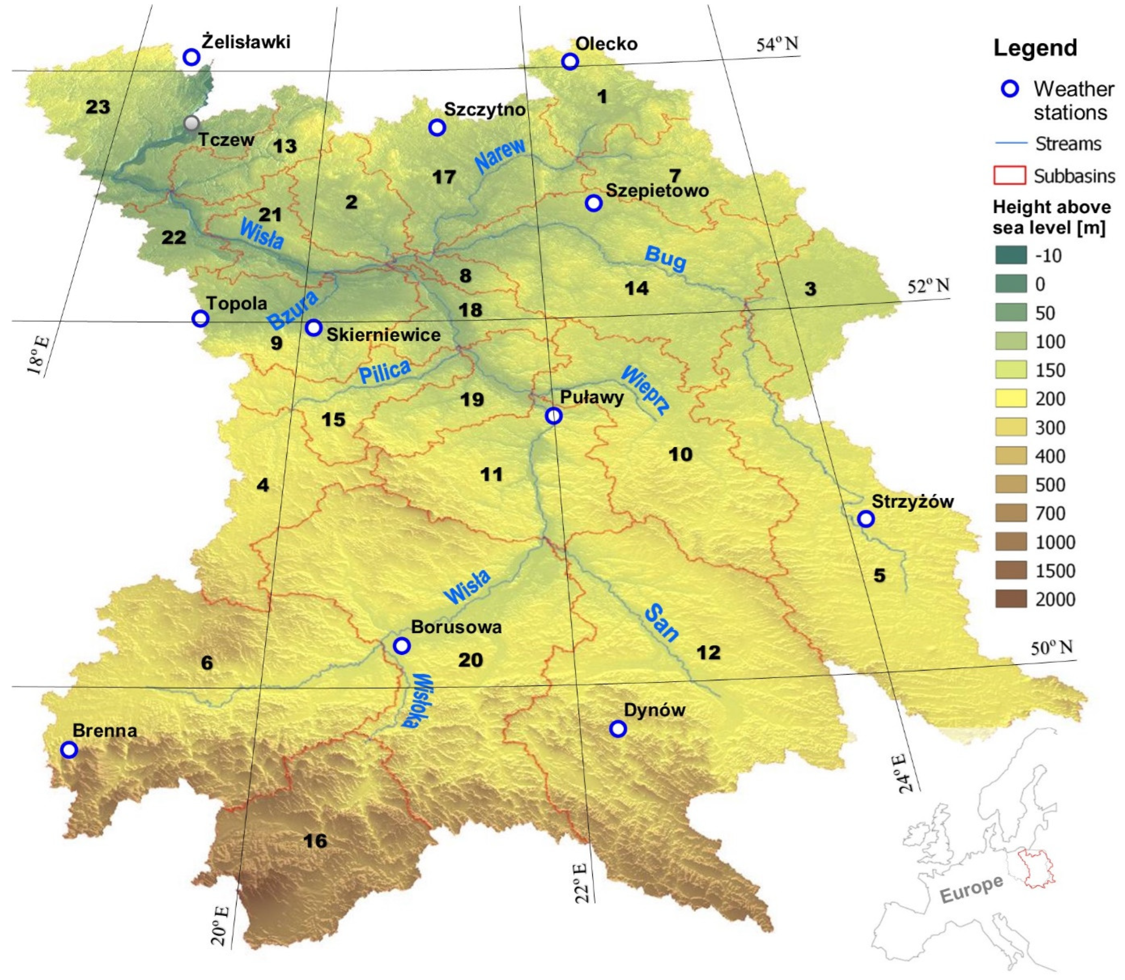
Poland, as a country, has modest water resources and ranks 24th in Europe in terms of the volume of renewable freshwater resources per capita—1600 m³, while per capita in Europe, there are 4011 m³ [1,4]. According to the United Nations (UN), water resources in Poland are below the water security level [4]. In addition, the area of Poland is characterised by high variability of water resources in time and space. The most scarce natural areas fed by precipitation are those located in the central belt of Poland [5]. The situation is different in submontane regions, where there is more precipitation. In these regions, excessive precipitation may contribute to flooding and waterlogging. In addition to spatial variability, there is high variability in precipitation, both annually and over many years. Under the climatic conditions of central Europe, the highest flows in watercourses usually occur in spring, while the lowest flows occur in summer and autumn. In recent years, variability in river outflows has been noticeable. Surface and groundwater levels have decreased significantly, causing droughts in many regions, while other areas often experience inundation, flooding, and floods [1].

The reason for this situation is most often economic activity, which in many cases has reduced the natural retention capacity of the catchment area. The rapid discharge of water in spring floods and after precipitation has worsened the structure of the water balance of Poland’s natural resources. Water scarcity is particularly acute during the growing season, especially when a dry summer is preceded by a snowless winter [1].

The second reason for the deterioration of the water balance structure is caused by increased water abstraction for municipal, industrial, and agricultural purposes. At present, agricultural production in Poland is based mainly on precipitation; only a negligible percentage of crops are irrigated [2], but in the near future, due to climate change, an increase in irrigation needs in field agricultural production, especially horticultural and orchard production, will be necessary. Under conditions of low freshwater resources in the near future, this may lead to an increasing dependence of food production on non-renewable water consumption. All the above-mentioned factors will worsen the water balance, which is why it is necessary to take a number of both preventive and intervention measures to ensure that water resources are used rationally [2]. There is, therefore, a natural need to make increasingly efficient use of existing water resources.

A worrying trend for agriculture is the observed changes in the distribution of rainfall over the year. Larger but less frequent precipitation events may cause many environmental changes, e.g., increase the risk of flooding, increase soil erosion, change the volume of surface runoff, alter water infiltration, and even increase the risk of agricultural drought. This is indicated by climate scenarios, according to which an increase in the variance of precipitation, up to 20%, is to be expected. According to Kundzewicz and Kozyra [6], climate models unanimously show that precipitation in some mid-latitude areas will decrease in the summer. However, projections of precipitation changes are characterised by high uncertainty. The geographical location of Poland means that wet air masses and snowfall have usually arrived in the winter. However, in recent years, snow cover in Poland has been decreasing. Its absence increases the frequency and duration of drought episodes, especially during the growing season, when we need water the most. Therefore, water resources may be less available in the 21st century.

To prepare for upcoming changes, including those affecting the Vistula River basin, it is essential to understand the impact of climate change on the environment, such as the occurrence of extreme weather events, droughts, and violent storms. Such knowledge is indispensable for developing solutions that mitigate the adverse effects of climate change [7,8].

There is growing interest in understanding the interactions between climate change and agricultural production, and this is motivating a significant amount of research [9].

A wide variety of studies are being conducted in Poland using the SWAT model, both for small catchments [10,11,12,13,14,15,16,17] and large catchments [18,19,20,21]. A paper on two small catchments, the Gąsawka and Rega, and one large catchment, the Warta, analysed the effect of catchment size on the calibration process and simulation results [18]. The peculiarities of hydrological phenomena occurring in Central Europe and the lack of sufficiently long measurement series for small catchments have a significant impact on the results obtained from the SWAT model for catchments in Poland [18].

Applying the SWAT hydrological model, the study examined the impact of climate change on water resources in the Central and Eastern European regions [21]. The research utilised a set of nine climate simulations from EURO-CORDEX, corrected for systematic errors, for the time horizons of 2024–2050 and 2074–2100 under two representative concentration pathways (RCPs), to forecast future water balance and streamflow conditions in the Vistula and Oder river basins. This comprehensive dataset can be valuable for scientists, water managers, and decision-makers in the water sector. However, the authors emphasise that the forecasts are subject to considerable uncertainty, as detailed in the documentation [21]. For the Vistula and Oder catchments, another study was conducted using the SWAT model [19,20].

In 2015, a publication on a high-resolution SWAT model addressing hydrology and water quality at a continental scale for Europe was released [22]. The study covered various large river basins in Europe, including Aare, Angermaelven, Danube, Dnieper, Duero, Ebro, Elbe, Garonne, Guadalquivir, Inn, Luleaelven, Loire, Maros, Northern Dvina, Oder, Olt, Pechora, Po, Rhine, Rhone, Sava, Siret, Szamos, Tiber, Thames, Tisza, Trent, Vistula, and Volga.

The research was motivated by the increasing impact of various factors on local, national, and regional water sources crucial for irrigation, energy production, industrial purposes, domestic use, and environmental conservation. Consequently, in many European regions, groundwater resources are diminishing and their quality is deteriorating. Climate change adds an additional challenge, introducing a new level of uncertainty regarding the availability of freshwater. The utilisation of large and precise water resource models facilitated a comprehensive investigation of integrated system behaviour through simulations based on physical data. The calibrated model and its outcomes can provide valuable information and support for water managers, particularly in Eastern European countries where rapid economic development may pose challenges related to freshwater availability [22].

The developed approach and methods in the study are general and can be applied to any large region worldwide [22].

The aim of this study is to analyse the hydrology of the Vistula River basin in climate projections for the years 2020–2050 under the climate change scenarios of RCP 4.5 and RCP 8.5 and to assess it in relation to the current state of knowledge related to research covering the European continent as well as small regional watersheds.

2. Study Area

The study area covers the Vistula River catchment area of 194,424 km². Most of the Vistula catchment is lowland, with an average catchment elevation of 270 m above sea level, with the highest point of the catchment being 2655 m above sea level in the Tatra Mountains [23]. The Vistula River flows longitudinally from the south, originating in mountainous regions and heading northward until it reaches the Baltic Sea [24].

The Vistula River catchment has the second-largest catchment area in the Baltic Sea basin [25] and is clearly asymmetrical. Its upper and middle reaches are dominated by right-bank tributaries. The part of the river network that is located in the upper reaches of the Vistula catchment, up to the mouth of the San, is characterised by high gradients and floods. The density of the river network in the aforementioned area is also greater than in the rest of the Vistula catchment. In the lower reaches of the Vistula basin, the distribution of the river network becomes uniform [23] (Figure 1).

The Vistula River catchment area is located in a temperate climate zone with transitional characteristics between the maritime and continental varieties, characterised by high variability in weather conditions [23,26]. According to the Atlas of Poland’s Climate for 1991–2020 [26], the average annual wind speed was 3.5 m/s for the study region. The average annual precipitation amounted to 678.6 mm, with an average precipitation of 117.8 mm in winter, 153.7 mm in spring, 247.1 mm in summer, and 160.0 mm in autumn. The average annual air temperature was 8.4 °C, with −1.4 °C in January and 18.4 °C in July. The average duration of the growing season was 224 days. The average annual relative humidity was 77% [26].

3. Methods and Data

For modelling the Vistula River basin, the SWAT model (the Soil and Water Assessment Tool) was employed [27].

The model was prepared using QSWAT 3 software (version 1.1) with an interface within Quantum GIS (version 3.10.13 Coruna) [28]. For the model calculations, SWAT Editor software (version 2012.10.23) was employed [29].

The programme allows processes to be simulated with different time resolutions: year, month, or day.

The following analyses (processes) were performed in the SWAT model:

-

surface runoff,

-

flow in the watercourse,

-

groundwater supply to watercourses,

-

infiltration,

-

aquifer recharge,

-

sediment transport in the catchment.

The SWAT model was also calibrated and validated using the SWAT CUP (SWAT Calibration and Uncertainty Programs) software (version 5.2.1) [22,30].

3.1. Data Collection

For this SWAT model, the following data were used:

-

numerical terrain model covering the catchment area at 50 m × 50 m resolution in the form of a DEM [31];

-

site hydrography data in the form of Shapefiles—rivers, lakes, catchments, and databases [32];

-

digital vectorised soil maps at scales of 1:100,000 and 1:500,000 in the form of Shapefiles and databases obtained from IUNG (the Institute of Soil Science and Plant Cultivation);

-

Digital Soil Map of the World and databases in the form of Shapefiles [33,34];

-

detailed Geological Map of Poland and databases [35];

-

land use database in the form of a Shapefiles [36];

-

daily meteorological data for 2008–2018 obtained from 11 weather stations as databases with precipitation (mm), temperature (°C), wind speed (m/s), humidity, and solar total radiation (MJ/m²) [37];

-

monthly average outflow (m³/s) for periods 2013–2016 (calibration) and 2017–2018 (validation).

3.2. Catchment Development and HRU Areas

Based on the numerical terrain model (50 m × 50 m) [31] and the hydrography of the area [32], the Vistula River catchments were divided into 23 sub-catchments (Figure 1).

Creating a SWAT model necessitates the incorporation of various input data, such as soil maps, slope maps, and land cover maps [27]. To create the soil database, digital soil-agricultural maps at scales of 1:100,000 and 1:500,000 were utilised, obtained from IUNG, along with geological data [35]. For the Vistula River basin area beyond Poland’s borders, the Digital Soil Map of the World [33] was used. A major problem in mapping soils and parameters characterising a soil type and soil type into the SWAT model is the discrepancies between the division of soils into granulometric groups [38] and that used in the SWAT model and the division of soils into granulometric groups by the Polish Soil Science Association [39,40]. In 2008, the Polish Soil Science Association introduced a new scheme for the division of soils into granulometric groups, PTG 2008 [41], fully in line with the division [38]. With PTG 2008, it is possible to compare the results of agronomic and soil surveys carried out in Poland with most foreign surveys.

CORINE Land Cover in a vector version with a reference scale of 1:100,000 was used to prepare the land use [36].

For the purposes of the SWAT model, data for particle size groups corresponding to the 2008 PTG [41] were entered in the physical soil parameters for the individual layers [42].

The soil database consists mainly of sandy soils of different genetic types. The largest area is occupied by AB—podzolic soils and brown soils (24%), as well as A—podzolic soils and clay-illuvial soils (22%). A large area is also occupied by Bw—rusty soils and acid brown soils (13%), B—ordinary brown soils (8%), and D—ordinary black earth (5%) (

Table 1. Classification by soil type and species, along with the percentage of soils in the Vistula River basin, was generated using the QSWAT interface (own study).

Type of Soil and Fraction	Part [%]	Type of Soil and Fraction	Part [%]	Type of Soil and Fraction	Part [%]	Type of Soil and Fraction	Part [%]	Type of Soil and Fraction	Part [%]
AB-gl	0.23	B-gl	3.87	Bw-pl	0.18	OJ-ps	0.04	Bd66-1-2b-3008	0.03
AB-gs	0.01	B-gs	0.44	Bw-pli	0.42	E-gl	0.09	Bd71-1-2b-6416	0.30
AB-pgl	2.09	B-i	0.13	Bw-plz	0.71	E-gs	0.03	Bd72-2b-3011	0.19
AB-pgl-gp	0.04	B-ls	1.79	Bw-plz-gs	0.24	E-ls	0.12	Be121-2bc-3014	0.56
AB-pgl-pl	1.84	B-pgl	0.08	Bw-plz-pl	0.33	E-pgl	0.13	Ch5-2a-3032	0.06
AB-pl	9.56	B-pgl-gl	0.32	Bw-ps	0.17	E-pl	0.07	Cl12-2ab-3041	0.57
AB-plz	0.27	B-pgm	0.04	Bw-ps-gs	0.05	E-plz	0.03	De18-1a-3048	0.00
AB-ps	7.88	B-pgm-gs	0.22	C-ls	1.00	E-ps	0.26	De18-2a-3049	0.33
AB-ps-gp	1.56	B-pl	0.09	D-gl	1.07	F-i	1.83	De19-2a-3051	1.61
AB-psp-ps	0.25	B-plz	0.53	D-gs	0.14	F-pgl-pl	0.04	Dg5-1ab-3055	0.04
A-gl	1.88	B-ps	0.40	D-gsp	0.05	F-plz	0.05	Gm14-2-3a-3068	1.19
A-gs	0.30	Bw-gc	0.24	D-i	0.05	F-plz-pl	0.06	I-U-1-2c-6532	0.22
A-ls	1.93	Bw-gcp	0.49	D-ls	0.04	F-ps	3.14	Je87-2-3a-3149	0.06
A-pgl	0.82	Bw-gl	0.92	D-pgl	1.07	G-gs	0.03	Lg40-2ab-6554	0.00
A-pgl-gl	4.44	Bw-glp	0.27	D-pgm	0.18	G-ls	0.05	Lg41-2-3a-3194	0.00
A-pgm	0.11	Bw-gs	0.34	D-pgm-gl	0.53	G-pgl	0.06	Lg41-2-3a-6555	0.00
A-pgm-gp	1.85	Bw-gsp	1.32	D-pgmp	0.11	G-plz	0.05	Lg54-1a-3198	2.08
A-pgmp-gp	0.97	Bw-i	0.19	D-pli	0.06	M-gl	0.08	Lg55-1a-3199	1.05
A-pgm-ps	0.05	Bw-ls	2.49	D-plz	0.17	M-pgl	0.08	Lo78-1-2a-3204	0.01
A-pl	1.06	Bw-pgl	0.35	D-plz-gl	0.09	M-pgl-ps	0.11	Lo89-2a-3207	0.10
A-plz	0.36	Bw-pgl-gl	2.67	D-plz-pl	0.20	M-pli	0.06	From22-a-3217	0.00
A-plz-gl	0.82	Bw-pgl-pl	0.46	D-ps	0.62	M-ps	2.92	Ph14-1-2c-6680	0.00
A-plz-ps	1.56	Bw-pgm	0.16	Dz-pgl	0.05	R	1.47	Pl5-1ab-3236	4.41
A-ps	5.83	Bw-pgm-gs	0.50	Dz-pgm	0.02	Tn	3.06	Po30-1ab-3239	0.00
A-ps-gl	0.13	Bw-pgmp	0.47	OJ-plz	0.07	W	1.04	E23-2bc-6494	0.00

, Figure 2). Other soil types within the Polish borders are Dz—black earth degraded and grey earth; E—peaty-muddy gleysols and muddy-peaty gleysols; F—alluvial soils; G—gleyic soils; M—murshic-mineral soils and semimurshic; R—soils; Tn—fen; and W—water [43]. Soils located outside Poland account for 13% of the drainage basin (Figure 2). A total of 125 particle-size groups were distributed. These are: Bd—dystric Cambisols, Be—Eutric Cambisols, Ch—Haplic Chemozems, Cl—Luvic Chemozems, De—Eutric Podzoluvisols, Dg—Gleyic Podzoluvisols, Gm—Mollic Gleysols, I-U—Lithosols–Rankers, Je Eutric Fluvisols, Lg—Gleyic Luvisols, Lo—Orthic Luvisols, Od—Dystric Histosols, Ph—Humic Podzols, Pl—Leptic Podzols, Po—Orthic—Podzols, E—Rendzinas [34,44].

The land use database of the Vistula basin has been compiled from the Corine Land Cover [36] databases (Figure 3).

Land use types denote, in turn (Figure 3,

Table 2. Classification by land cover type, along with the percentage distribution of land cover in the Vistula River basin, was generated using the QSWAT interface (own study).

CLC CODE	SWAT CODE	Area [ha]	Part [%]	CLC CODE	SWAT CODE	Area [ha]	Part [%]
111	URHD	192,853	1.02	242	AGRL	705,744	3.71
112	URML	711,405	3.74	243	CRGR	734,976	3.87
121	UCOM	188,235	0.99	311	FRSD	1,248,111	6.57
124	UTRN	109,861	0.58	312	FRSE	2,655,099	13.97
131	UIDU	88,786	0.47	313	FRST	1,567,429	8.25
133	URLD	70,331	0.37	321	RNGE	209,436	1.1
142	FESC	507,606	2.67	324	SHRB	164,516	0.87
211	CRDY	7,088,468	37.3	333	BSVG	65,501	0.34
222	ORCD	847,624	4.46	411	WEHB	86,347	0.45
231	PAST	1,614,573	8.49	511	WATR	149,327	0.79

): URHD (111)—continuous urban fabric, URML (112)—discontinuous urban fabric, UCOM (121)—industrial or commercial units, UTRN (124)—airports, UIDU (131)—mineral extraction sites, URLD (133)—construction sites, FESC (142)—sport and leisure facilities, CRDY (211)—non-irrigated arable land, ORCD (222)—fruit trees and berry plantations, PAST (231)—pastures, AGRL (242)—complex cultivation patterns, CRGR (243)—land principally occupied by agriculture, with significant areas of natural vegetation, FRSD (311)—broad-leaved forest, FRSE (312)—coniferous forest, FRST (313)—mixed forest, RNGE (321)—natural grasslands, SHRB (324)—transitional woodland shrub, BSVG (333)—sparsely vegetated areas, WEHB (411)—inland marshes, WATR (511)—water [36].

Arable land (58%) and forests (29%) predominate in the Vistula River basin (Table 2). Anthropogenic land accounts for 10%. The majority of agricultural land consists of non-irrigated arable land (37%), while meadows and pastures (8%), orchards, and plantations (4%) also account for a large area.

The topography of the Vistula River basin has been divided similarly to that of the Bystrej River basin [45]. A total of 86% of the basin’s area consists of terrain with slopes up to 6%; 6% of the basin’s area is made up of slopes ranging from 6 to 10%; 6% of the basin’s area consists of slopes ranging from 10 to 27%; and 2% of the basin’s area consists of slopes exceeding 27%. Next, 1055 Hydrologic Response Units (HRUs) were generated [27].

3.3. Development of Meteorological Databases

In the next stage, daily meteorological data for the years 2008–2018, obtained from statutory research conducted by IUNG and IMGW [37], were incorporated into the SWAT model. The data were prepared using SWATWeather Database software (version 0.18.03) [46]. In total, data were collected from 11 meteorological stations: Borusowa, Brenna, Dynów, Olecko, Puławy, Skierniewice, Strzyżów, Szepietowo, Szczytno, Topola, and Żelisławki (Figure 1).

Additionally, some parameters for point source discharges [47] were corrected and supplemented, along with hydrography data [32]. River parameters in the catchments were also corrected, as the automatically generated river parameters for river length, depth, and width were overestimated [32,37].

The current CO concentration value was also entered into the prepared SWAT model.

3.4. Use of the SWAT-CUP Programme

After inputting all the necessary data into the SWAT model, the water cycle in the Vistula River basin was simulated for the years 2008–2018 with a five-year warm-up period. After the SWAT simulation, the resulting model was calibrated in SWAT-CUP [30,48,49].

As the elevation differences in the Vistula basin are large, the elevation-band programme in SWAT-CUP divided the catchments with the largest elevation differences into five bands. This division into elevation bands allowed each band to be simulated separately, which allowed for a better fit in the SWAT-CUP model’s simulation of precipitation and temperature.

The calibration of the model utilised data from the years 2013 to 2016 with monthly flow rates from the measurement station in Tczew. Once satisfactory calibration was achieved, the model was validated on a 2-year dataset (2017–2018).

After sensitivity analysis and calibration (500 iterations), the results obtained were within satisfactory ranges [48,50] (Figure 4). The sensitivity of the 13 input parameters (ALPHA_BF.gw, CN2.mgt, ESCO.hru, EPCO.hru, GW_DELAY.gw, GWQMN.gw, GW_REVAP.gw, REVAPMN.gw, RCHRG_DP.gw, SOL_AWC().sol, SOL_BD().sol, SOL_K().sol, SOL_Z().sol) was analysed using the SUFI-2 algorithm in the SWAT Calibration Uncertainties Programme (SWAT CUP).

4. Climate Change Scenarios

For assessing the water balance of the Vistula River basin, three RCMs (regional climate models) driven by a GCM (global climate model) were selected, considering two RCP (representative concentration pathways) scenarios [51]. The data were obtained and prepared in a similar manner to the SWAT model for the Bystra River basin [45]. The daily data of the analysed climate scenarios for the period 2020–2050 were extracted from the EURO-CORDEX database [52,53]. The spatial extent of the data obtained covered the European area with a resolution of 0.11°. Temperature and precipitation were adjusted by SMHI (the Swedish Meteorological and Hydrological Institute) using DBS (distribution-based scaling) [54] and MESAN (the regional MESoscale Analysis) methods [55]. Additionally, the CDO (Climate Data Operators) software (version 1.7.0) was used to set the correct geographic longitude and latitude [56].

Climate change scenarios RACMO22E, HIRHAM5, and RCA4 were selected due to their distinct parameterisation of physical processes occurring within the same spatial domain covering the European continent. These three models are based on the boundary and initial conditions of the same global model (EC-EARTH).

The data obtained from the climate scenarios were compiled into databases for the same meteorological stations used to run the SWAT model (methodology chapter) (

Table 3. Brief description of climate projections for radiative forcing (own study).

Model Variant	General Circulation Model (GCM)	Regional Climate Models (RCM)	Short Name of Models
			RCP 4.5 (+4.5 Wm−2)	RCP 8.5 (+8.5 Wm−2)
ICHEC-EC-EARTH_KNMI-RACMO22E	EC-EARTH	RACMO22E	RCP 4.5.A	RCP 8.5.A
ICHEC-EC-EARTH_DMI-HIRHAM5	EC-EARTH	HIRHAM5	RCP 4.5.B	RCP 8.5.B
ICHEC-EC-EARTH_SMHI-RCA4	EC-EARTH	RCA4	RCP 4.5.C	RCP 8.5.C

). RCP 4.5 entails the implementation of new technologies to achieve a higher reduction in greenhouse gas emissions than the current level. On the other hand, RCP 8.5 signifies the continuation of the current pace of greenhouse gas emissions growth [57].

5. Results of the Application of RCP 4.5 and RCP 8.5 for 2020–2050

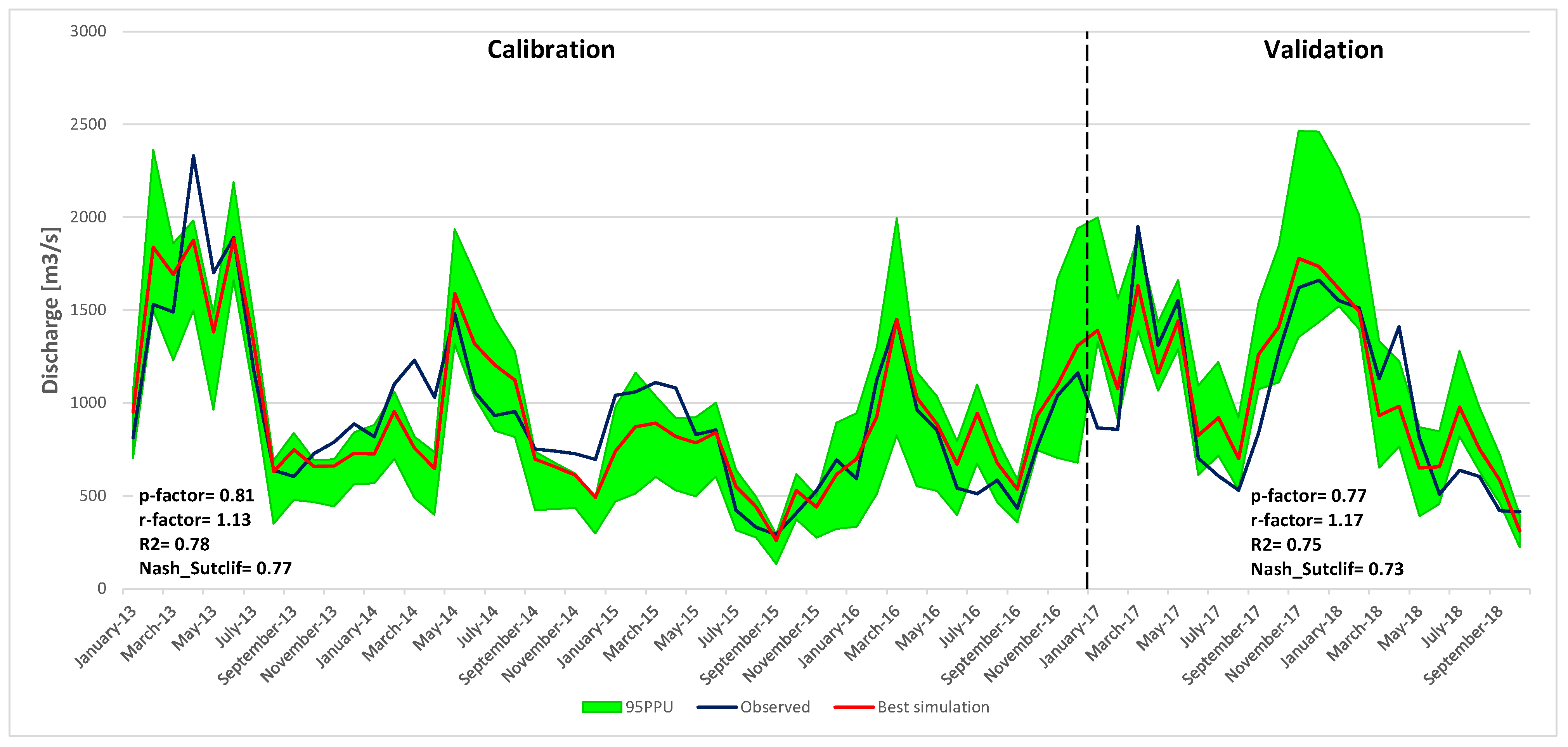
After calibration and validation of the SWAT model, flow simulations were carried out for the Vistula catchment for two climate scenarios and three models for the period 2020–2050.

To compare climate change scenarios for individual forecasts, a single iteration was conducted in SWAT-CUP using the best calibration parameters. In addition, for the RCP 4.5 and RCP 8.5 scenarios, changes in CO₂ concentrations were assumed for each decade: from 2021 to 2030, from 2031 to 2040, and from 2041 to 2050, as developed by the Potsdam Institute for Climate Impact Research [58,59].

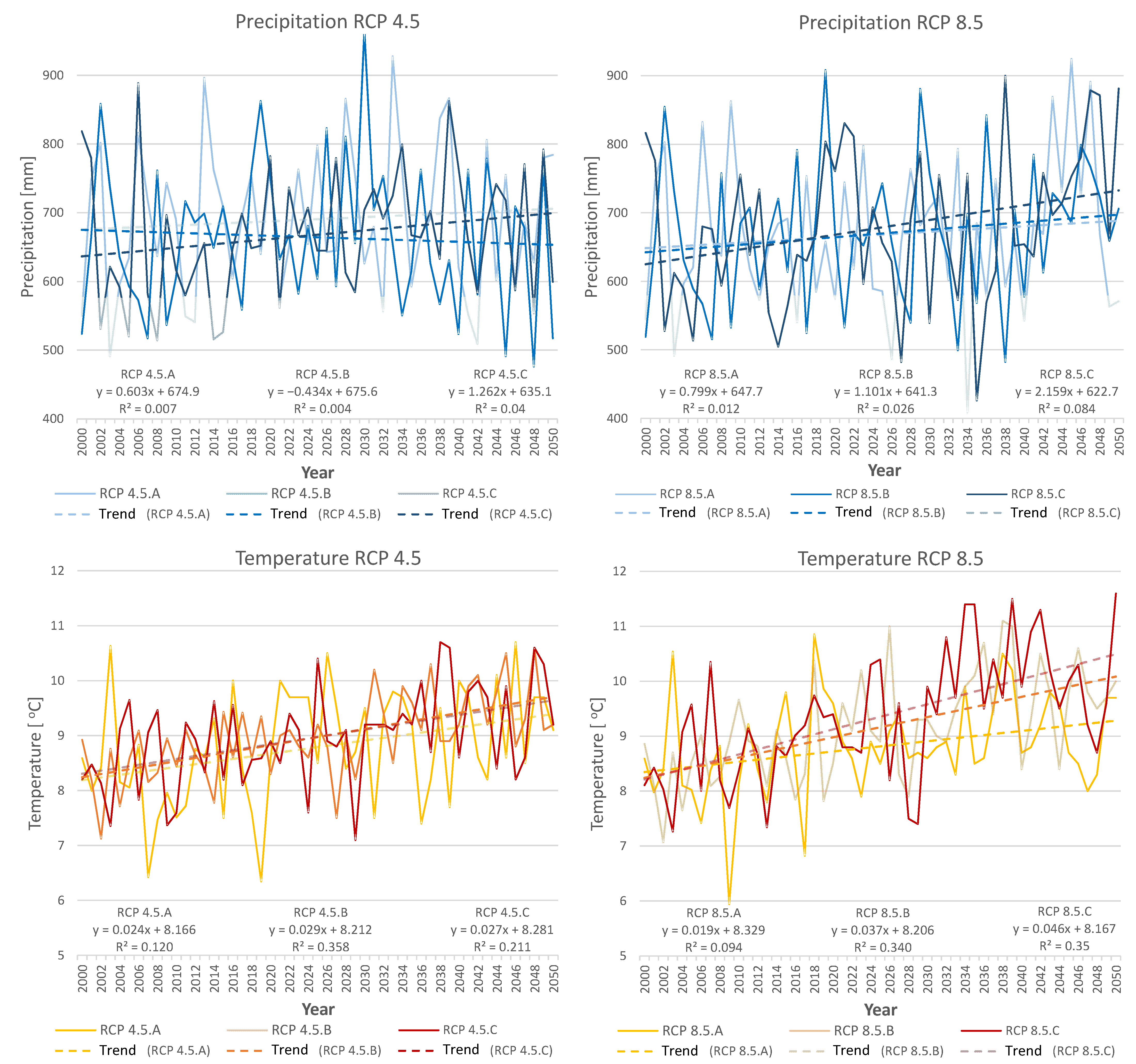
Average annual precipitation totals for most projections (except the RCP 4.5.C) will show an increasing trend in the following decades (Figure 5).

In the upcoming decades, the average annual temperature is expected to rise in all three projections for both the RCP 4.5 and RCP 8.5 scenarios.

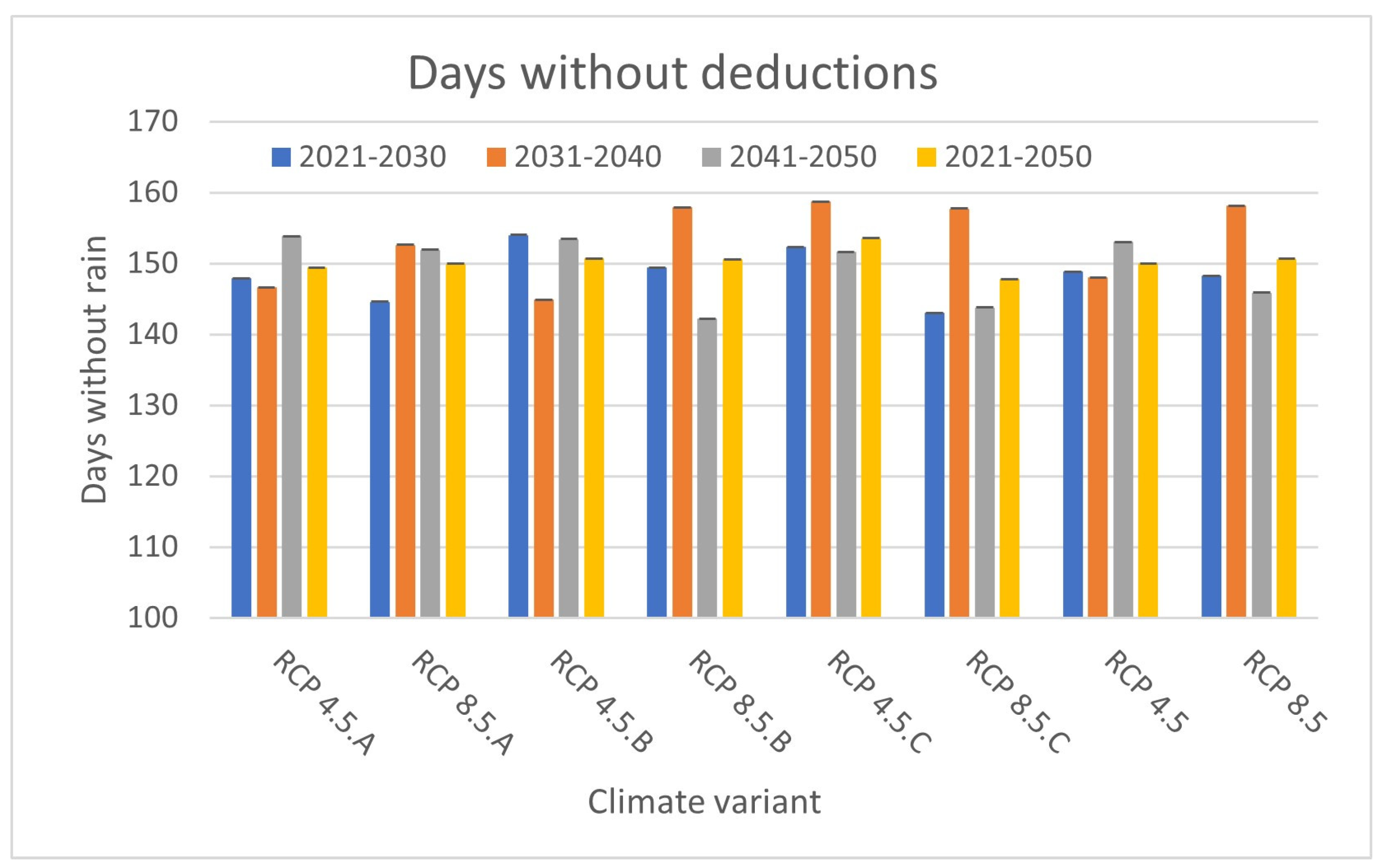
The annual average number of days without precipitation shows a clear downward trend in RCP 8.5.A. On the other hand, a clear upward trend is visible in RCP 4.5.B. In the other projections, the trend changes minimally over the next few years (Figure 6 and Figure 7).

The annual average number of days with a mean temperature above 5 °C in the coming decades will increase significantly for most forecasts, with the exception of RCP 4.5.A, where the trend will be downward.

The mean seasonal precipitation totals for the Vistula catchment in the 2013–2018 simulation years change compared to the individual climate change projections in 2021–2030, 2031–2040, and 2041–2050 (

Table 4. Comparison of precipitation for different seasons during the SWAT simulation period (2013–2018) with climate projections (RCP 4.5.A, RCP 4.5.B, RCP 4.5.C, RCP 8.5.A, RCP 8.5.B, and RCP 8.5.C) for the years 2021–2030, 2031–2040, and 2041–2050 in the Vistula River basin. Shaded dark red figures indicate a large percentage decrease in rainfall, and shaded light red figures indicate a small percentage decrease in rainfall. Shaded dark blue numerals indicate a large percentage increase in precipitation, and shaded light blue numerals indicate a small percentage increase in precipitation (own study).

Climate Scenario		RCP 4.5			RCP 8.5
Climate Projection	Model 2013–2018	RCP 4.5.A	RCP 4.5.B	RCP 4.5.C	RCP 8.5.A	RCP 8.5.B	RCP 8.5.C
Season		Average seasonal precipitation [mm]
Time interval	2021–2030
DJF	105	101	115	118	105	105	121
		−4%	+10%	+12%	+1%	0%	+16%
MAM	155	154	159	155	155	149	179
		−1%	+2%	0%	0%	−4%	+15%
JJA	198	276	263	240	267	250	200
		+39%	+33%	+21%	+35%	+26%	+1%
SON	166	166	164	151	136	167	173
		0%	−1%	−9%	−18%	0%	+4%
Average annual	624	697	702	664	663	671	673
		+12%	+12%	+6%	+6%	+8%	+8%
Time interval	2031–2040
DJF	105	117	116	118	89	113	124
		+11%	+10%	+13%	−15%	+7%	+18%
MAM	155	162	136	168	166	128	180
		+4%	−12%	+8%	+7%	−18%	+16%
JJA	198	283	254	251	241	247	213
		+43%	+28%	+27%	+22%	+25%	+8%
SON	166	159	133	187	137	146	138
		−4%	−20%	+13%	−17%	−12%	−17%
Average annual	624	720	639	724	633	634	655
		+15%	+2%	+16%	+1%	+2%	+5%
Time interval	2041–2050
DJF	105	105	117	116	110	116	153
		0%	+11%	+11%	+5%	+11%	+46%
MAM	155	156	158	167	201	184	178
		0%	+2%	+8%	+29%	+19%	+15%
JJA	198	256	221	217	253	246	220
		+29%	+12%	+9%	+28%	+24%	+11%
SON	166	153	148	169	166	172	212
		−8%	−11%	+2%	0%	+4%	+28%
Average annual	624	669	644	669	730	718	763
		+7%	+3%	+7%	+17%	+15%	+22%

). These changes are particularly evident in the JJA (June, July, and August) season, where an increase in precipitation is observed in all projections. For most projections, an increase in seasonal average precipitation is also seen in DJF (December, January, and February) and MAM (March, April, and May). The exception is the SON (September, October, November) season, where reductions in rainfall occur most frequently, up to 20%. For the RCP 4.5.C, RCP 8.5.B, and RCP 8.5.C projections, the seasonal mean precipitation is higher in most seasons than in the 2013–2018 simulation years.

The average annual precipitation for all projections in 2021–2030, 2031–2040, and 2041–2050 will be up to 22% higher (projection RCP 8.5.C—2041–2050) compared to the simulation years 2013–2018.

The average seasonal temperature patterns within the Vistula catchment during the 2013–2018 simulation years also exhibit changes when compared to the individual climate change projections for 2021–2030, 2031–2040, and 2041–2050 (

Table 5. Comparison of temperature for different seasons during the SWAT simulation period (2013–2018) with climate projections (RCP 4.5.A, RCP 4.5.B, RCP 4.5.C, RCP 8.5.A, RCP 8.5.B, and RCP 8.5.C) for the years 2021–2030, 2031–2040, and 2041–2050 in the Vistula River basin. Shaded dark red digits indicate a large percentage increase in temperature, and shaded light red digits indicate a small percentage increase in temperature. Shaded dark green digits indicate a large percentage decrease in temperature, and shaded light green digits indicate a small percentage decrease in temperature (own study).

Climate Scenario		RCP 4.5			RCP 8.5
Climate Projection	Model 2013–2018	RCP 4.5.A	RCP 4.5.B	RCP 4.5.C	RCP 8.5.A	RCP 8.5.B	RCP 8.5.C
Season		Average seasonal temperature distribution [°C]
Time interval	2021–2030
DJF	−0.2	0.6	−0.5	−1.7	−1.2	−0.3	−0.8
		+0.7	−0.4	−1.5	−1.0	−0.2	−0.7
MAM	8.9	10.1	7.5	9.3	10.2	9.1	8.6
		+1.2	−1.4	+0.4	+1.3	+0.2	−0.3
JJA	18.6	18.3	18.3	18.8	17.9	18.8	18.4
		−0.3	−0.3	+0.2	−0.7	+0.2	−0.2
SON	9.3	8.6	9.4	8.6	9.4	9.3	9.4
		−0.7	+0.1	−0.7	+0.1	0.0	+0.1
Average annual	9.2	9.4	8.7	8.8	9.1	9.2	8.9
		+0.2	−0.5	−0.4	−0.1	0.0	−0.3
Time interval	2031–2040
DJF	−0.2	−1.6	0.1	0.8	−0.2	0.5	1.5
		−1.4	+0.3	+0.9	−0.1	+0.7	+1.7
MAM	8.9	9.1	8.7	9.4	10.3	9.5	10.0
		+0.2	−0.2	+0.5	+1.4	+0.6	+1.1
JJA	18.6	18.7	19.0	18.6	18.4	19.4	19.5
		+0.1	+0.4	0.0	−0.2	+0.8	+0.9
SON	9.3	8.9	9.6	9.0	9.7	9.6	10.3
		−0.4	+0.3	−0.3	+0.4	+0.3	+1.0
Average annual	9.2	8.8	9.3	9.4	9.5	9.8	10.3
		−0.4	+0.2	+0.3	+0.4	+0.6	+1.2
Time interval	2041–2050
DJF	−0.2	−0.9	0.6	−0.1	−0.5	0.6	1.2
		−0.8	+0.8	+0.1	−0.3	+0.8	+1.4
MAM	8.9	10.0	9.2	9.0	10.0	9.0	9.9
		+1.1	+0.3	+0.1	+1.1	+0.1	+1.0
JJA	18.6	18.8	19.1	19.2	18.5	19.1	19.2
		+0.2	+0.4	+0.5	−0.1	+0.5	+0.6
SON	9.3	9.1	9.5	9.6	9.5	10.1	10.0
		−0.2	+0.2	+0.3	+0.2	+0.8	+0.7
Average annual	9.2	9.2	9.6	9.4	9.4	9.7	10.1
		+0.1	+0.4	+0.3	+0.2	+0.5	+0.9

). These changes are particularly pronounced in 2031–2040 and 2041–2050, where, for most seasons in all projections, the seasonal mean temperature will be higher than in the SWAT 2013–2018 simulation period. The highest increases (up to 1.4 °C) in temperature are recorded for the MAM season for all decades. The highest increases in annual mean temperature (up to 1.2 °C) are recorded for RCP 8.5.B and RCP 8.5.C projections for 2031–2040 and 2041–2050 compared to the simulation period (2013–2018).

The average annual temperature for most climate projections for 2021–2030 will fall to as low as 8.7 °C (RCP 4.5.B) compared to the 2013–2018 simulation period (9.2 °C). In contrast, for all projections in 2031–2040 and 2041–2050, the average annual temperature will increase to as much as 10.3 °C (RCP 8.5.C).

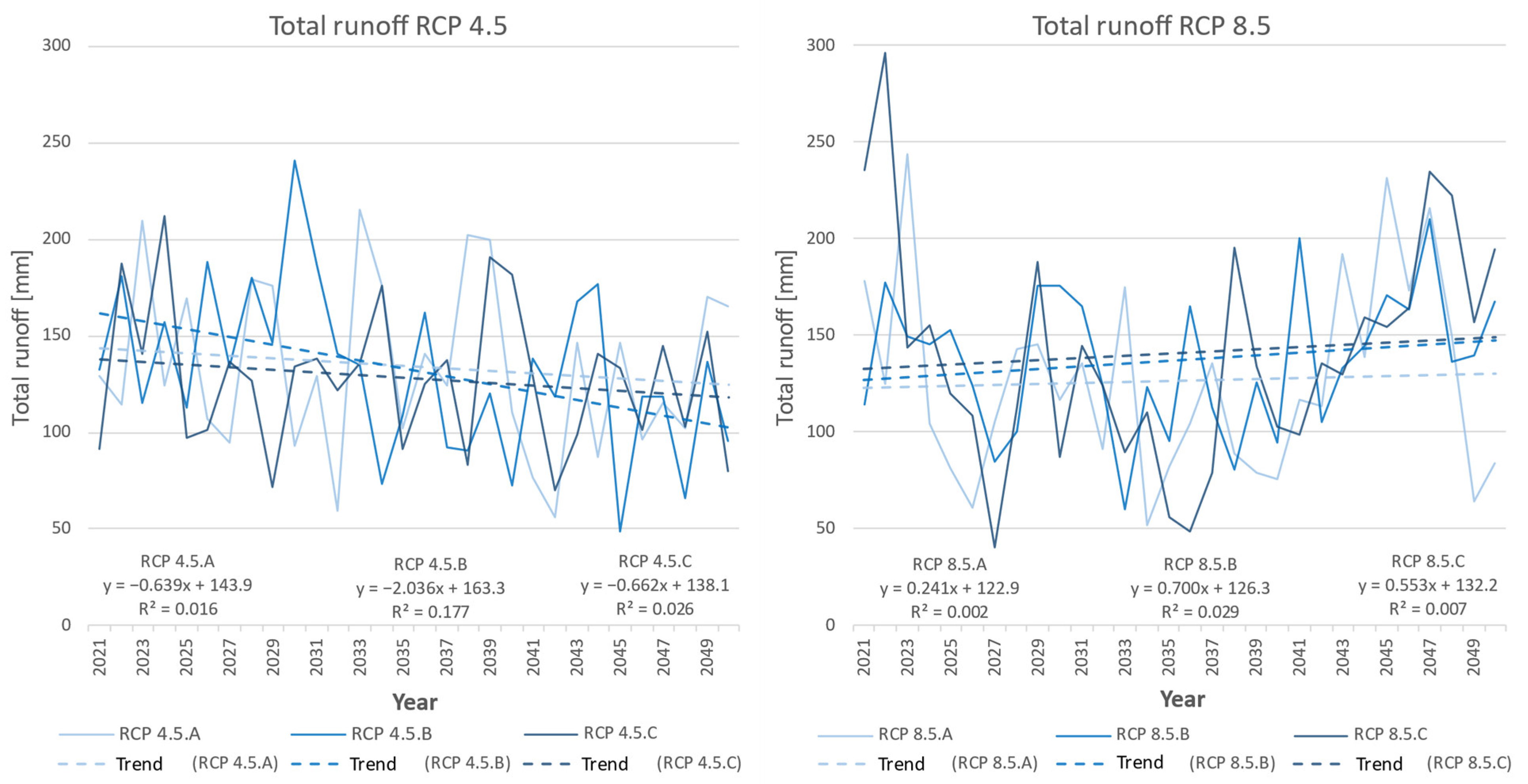
In all projections for the RCP 8.5 scenario, the average annual total runoff will trend upwards (Figure 8). The trend in annual total runoff will be similar.

The seasonal average total runoff for the Vistula catchment is expected to be higher for the majority of climate change projections in 2021–2030, 2031–2040, and 2041–2050 when compared to the simulation years of 2013–2018 (

Table 6. Comparison of total runoff for different seasons during the SWAT simulation period (2013–2018) with climate projections (RCP 4.5.A, RCP 4.5.B, RCP 4.5.C, RCP 8.5.A, RCP 8.5.B, and RCP 8.5.C) for the years 2021–2030, 2031–2040, and 2041–2050 in the Vistula River basin. Shaded dark red digits indicate a large percentage decrease in total runoff, and shaded light red digits indicate a small percentage decrease in total runoff. Shaded dark blue digits indicate a large percentage increase in total runoff, and shaded light blue digits indicate a small percentage increase in total runoff (own study).

Climate Scenario		RCP 4.5			RCP 8.5
Climate Projection	Model 2013–2018	RCP 4.5.A	RCP 4.5.B	RCP 4.5.C	RCP 8.5.A	RCP 8.5.B	RCP 8.5.C
Season		Average seasonal total runoff [mm]
Time interval	2021–2030
DJF	34	35	38	31	26	36	39
		+2%	+13%	−8%	−23%	+6%	+14%
MAM	34	31	47	43	36	40	50
		−10%	+36%	+25%	+4%	+17%	+45%
JJA	25	42	47	35	43	40	33
		+68%	+90%	+42%	+73%	+60%	+33%
SON	23	33	26	20	26	24	27
		+44%	+16%	−10%	+13%	+7%	+19%
Average annual	116	140	159	130	130	140	149
		+21%	+37%	+12%	+13%	+21%	+28%
Time interval	2031–2040
DJF	34	34	29	37	21	30	27
		0%	−13%	+10%	−38%	−11%	−22%
MAM	34	37	36	36	27	30	34
		+8%	+4%	+5%	−20%	−12%	−2%
JJA	25	48	32	34	33	36	31
		+93%	+29%	+38%	+31%	+47%	+25%
SON	23	27	21	30	21	18	17
		+18%	−8%	+34%	−9%	−21%	−25%
Average annual	116	146	118	138	102	115	108
		+26%	+2%	+19%	−12%	−1%	−6%
Time interval	2041–2050
DJF	34	29	28	32	37	33	52
		−15%	−17%	−4%	+10%	−2%	+53%
MAM	34	29	38	35	41	48	45
		−15%	+11%	+2%	+20%	+39%	+31%
JJA	25	34	29	28	38	45	30
		+37%	+18%	+14%	+54%	+83%	+21%
SON	23	24	23	19	31	30	38
		+7%	+1%	−14%	+37%	+34%	+68%
Average annual	116	116	118	115	148	157	165
		0%	+2%	0%	+28%	+36%	+42%

). The exception is the DJF season in 2041–2050, where, for most projections, the total runoff will be lower. In contrast, for the JJA season for all decades, the total runoff will be higher by up to 93% compared to the SWAT 2013–2018 simulation.

The average annual total runoff for most projections in the following decades (2021–2030, 2031–2040, 2041–2050) will increase up to 159 mm (RCP 4.5.B—2021–2030) compared to the 2013–2018 simulation period—116 mm.

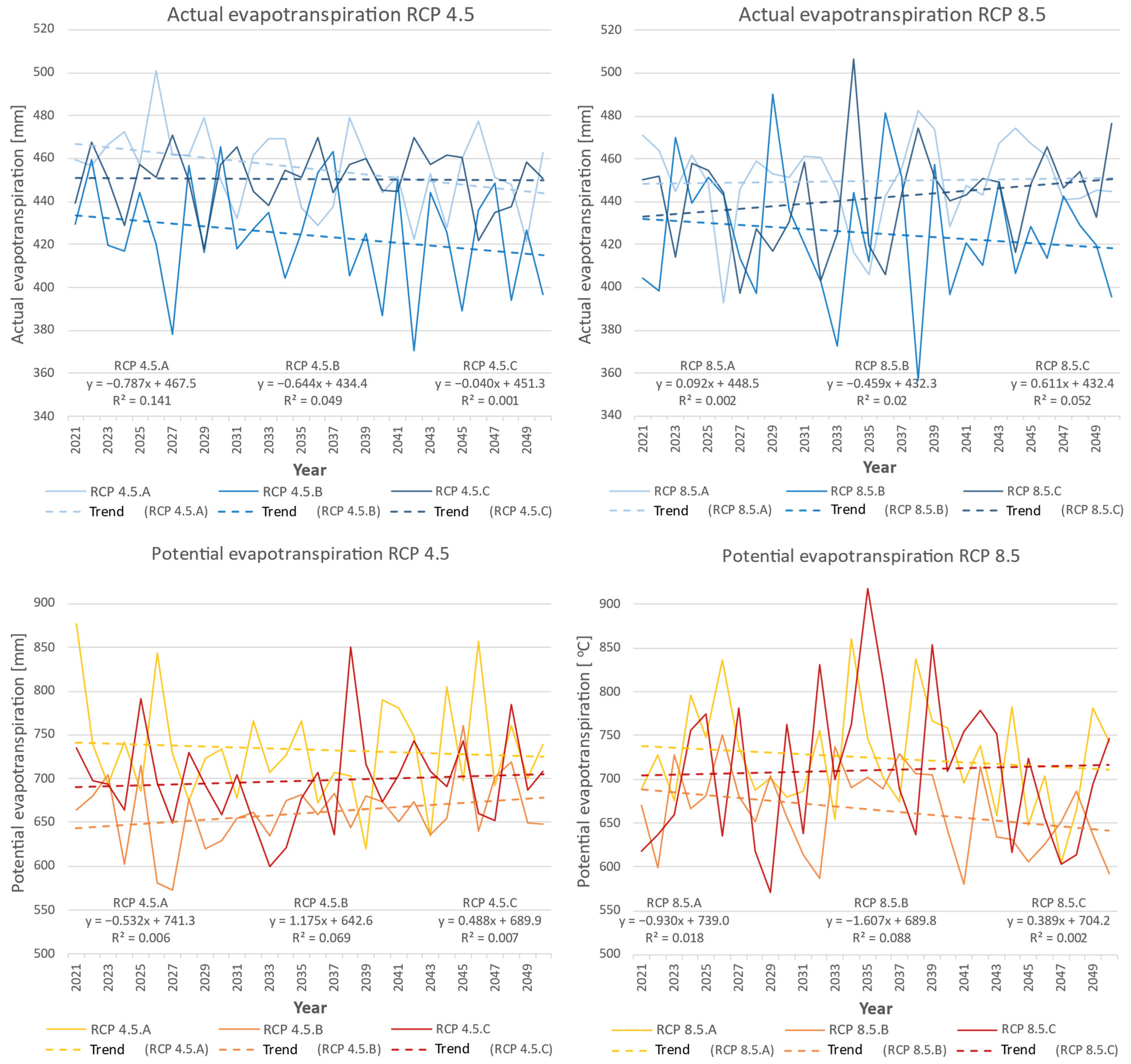
The trend line for the annual average of potential evapotranspiration in the climate change scenarios RCP 4.5.A, RCP 8.5.A, and RCP 8.5.B is expected to show a slight decrease in the upcoming decades (Figure 9). Conversely, in the climate change scenarios RCP 4.5.C, RCP 8.5.C, and RCP 4.5.B, the annual average of potential evapotranspiration is projected to increase in the future decades.

The trend in the annual average sum of actual evapotranspiration from 2020 to 2050 changes marginally across all projections.

Seasonal mean current evapotranspiration increases for most projections in all seasons compared to the 2013–2018 simulation period, with the highest increases occurring in the DJF and SON seasons (

Table 7. Comparison of actual evapotranspiration for different seasons during the SWAT simulation period (2013–2018) with climate projections (RCP 4.5.A, RCP 4.5.B, RCP 4.5.C, RCP 8.5.A, RCP 8.5.B, and RCP 8.5.C) for the years 2021–2030, 2031–2040, and 2041–2050 in the Vistula River basin. Shaded dark red digits indicate a large percentage decrease in actual evapotranspiration, and shaded light red digits indicate a small percentage decrease in actual evapotranspiration. Shaded dark blue digits indicate a large percentage increase in actual evapotranspiration, and shaded light blue digits indicate a small percentage increase in actual evapotranspiration (own study).

Climate Scenario		RCP 4.5			RCP 8.5
Climate Projection	Model 2013–2018	RCP 4.5.A	RCP 4.5.B	RCP 4.5.C	RCP 8.5.A	RCP 8.5.B	RCP 8.5.C
Season		Average seasonal actual evapotranspiration [mm]
Time interval	2021–2030
DJF	17	28	23	26	22	24	26
		+69%	+39%	+54%	+30%	+44%	+54%
MAM	119	136	119	121	131	122	125
		+14%	0%	+1%	+10%	+2%	+4%
JJA	209	224	213	226	220	216	210
		+7%	+2%	+8%	+5%	+3%	0%
SON	56	78	76	77	76	73	74
		+39%	+34%	+36%	+36%	+29%	+31%
Average annual	401	467	431	449	449	434	434
		+16%	+7%	+12%	+12%	+8%	+8%
Time interval	2031–2040
DJF	17	23	21	31	25	25	30
		+38%	+27%	+84%	+48%	+51%	+80%
MAM	119	131	120	126	132	117	129
		+9%	0%	+5%	+11%	−2%	+8%
JJA	209	221	207	220	215	206	214
		+6%	−1%	+5%	+3%	−1%	+2%
SON	56	77	76	76	75	71	70
		+38%	+36%	+35%	+34%	+26%	+24%
Average annual	401	452	424	453	447	420	443
		+13%	+6%	+13%	+11%	+5%	+10%
Time interval	2041–2050
DJF	17	22	23	27	23	22	31
		+33%	+35%	+59%	+39%	+29%	+83%
MAM	119	130	126	123	135	120	129
		+9%	+5%	+3%	+13%	+1%	+8%
JJA	209	219	200	222	217	206	212
		+5%	−4%	+6%	+4%	−1%	+2%
SON	56	76	70	78	78	74	77
		+35%	+24%	+39%	+39%	+31%	+37%
Average annual	401	448	418	450	453	422	448
		+11%	+4%	+12%	+13%	+5%	+12%

).

The average annual actual evapotranspiration for all projections in 2021–2030, 2031–2040, and 2041–2050 will increase up to 467 mm (RCP 4.5.A—2021–2030) compared to the 2013–2018 simulation period of 401 mm.

For potential evapotranspiration as well, the seasonal mean totals are anticipated to increase in most projections across all seasons when compared to the 2013–2018 simulation period, with the most significant increases occurring in the DJF and SON seasons. (

Table 8. Comparison of potential evapotranspiration for different seasons during the SWAT simulation period (2013–2018) with climate projections (RCP 4.5.A, RCP 4.5.B, RCP 4.5.C, RCP 8.5.A, RCP 8.5.B, and RCP 8.5.C) for the years 2021–2030, 2031–2040, and 2041–2050 in the Vistula River basin. Shaded dark red digits indicate a large percentage decrease in potential evapotranspiration, and shaded light red digits indicate a small percentage decrease in potential evapotranspiration. Shaded dark blue digits indicate a large percentage increase in potential evapotranspiration, and shaded light blue digits indicate a small percentage increase in potential evapotranspiration (own study).

Climate Scenario		RCP 4.5			RCP 8.5
Climate Projection	Model 2013–2018	RCP 4.5.A	RCP 4.5.B	RCP 4.5.C	RCP 8.5.A	RCP 8.5.B	RCP 8.5.C
Season		Average seasonal potential evapotranspiration [mm]
Time interval	2021–2030
DJF	20	39	30	33	29	33	33
		+92%	+45%	+63%	+42%	+60%	+61%
MAM	189	241	188	204	234	207	189
		+28%	0%	+8%	+24%	+10%	0%
JJA	326	349	320	352	343	336	351
		+7%	−2%	+8%	+5%	+3%	+8%
SON	81	115	107	112	122	103	109
		+42%	+32%	+38%	+50%	+27%	+35%
Average annual	616	744	644	701	728	679	681
		+21%	+5%	+14%	+18%	+10%	+11%
Time interval	2031–2040
DJF	20	30	27	38	35	33	39
		+46%	+32%	+87%	+73%	+60%	+93%
MAM	189	226	207	202	234	211	210
		+19%	+9%	+7%	+24%	+12%	+11%
JJA	326	344	323	338	347	330	374
		+6%	−1%	+4%	+7%	+1%	+15%
SON	81	114	108	106	128	106	132
		+40%	+33%	+30%	+58%	+31%	+63%
Average annual	616	714	665	684	744	680	755
		+16%	+8%	+11%	+21%	+10%	+23%
Time interval	2041–2050
DJF	20	30	29	34	29	27	38
		+48%	+42%	+66%	+44%	+32%	+87%
MAM	189	236	213	194	218	188	198
		+25%	+12%	+2%	+15%	0%	+5%
JJA	326	361	329	359	340	318	345
		+11%	+1%	+10%	+4%	−2%	+6%
SON	81	114	103	122	115	103	113
		+41%	+27%	+51%	+42%	+27%	+39%
Average annual	616	741	673	708	702	636	694
		+20%	+9%	+15%	+14%	+3%	+13%

).

The average annual potential evapotranspiration for all projections in 2021–2030, 2031–2040, and 2041–2050 will increase up to 755 mm (RCP 8.5.C—2031–2040) compared to the 2013–2018 simulation period—616 mm.

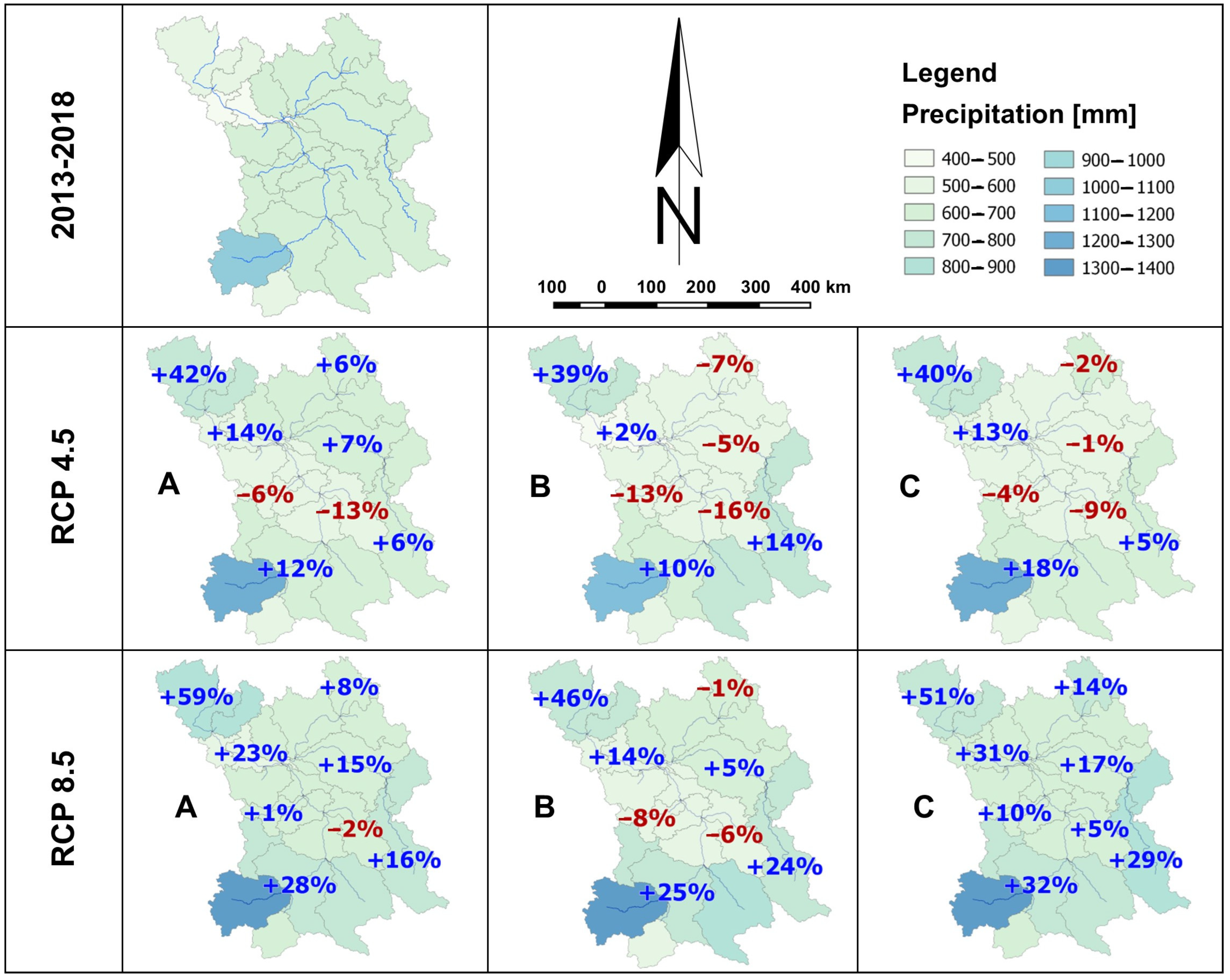
When analysing the spatial distribution of changes in mean annual precipitation across the 23 sub-catchments from the 2013–2018 simulation period to the 2041–2050 period (Figure 10) in the individual climate projections of RCP 4.5 and RCP 8.5 in the Northwest, South, and East regions, precipitation is expected to increase by several tens of percent. Increased average annual precipitation in most sub-basins between 2041 and 2050 will occur in the climate projections and RCP 8.5.B for the RCP 8.5 scenario. On the other hand, for all projections in the RCP 4.5.B scenario between 2041 and 2050, precipitation in the central region of the Vistula basin will be reduced by up to 16 percent.

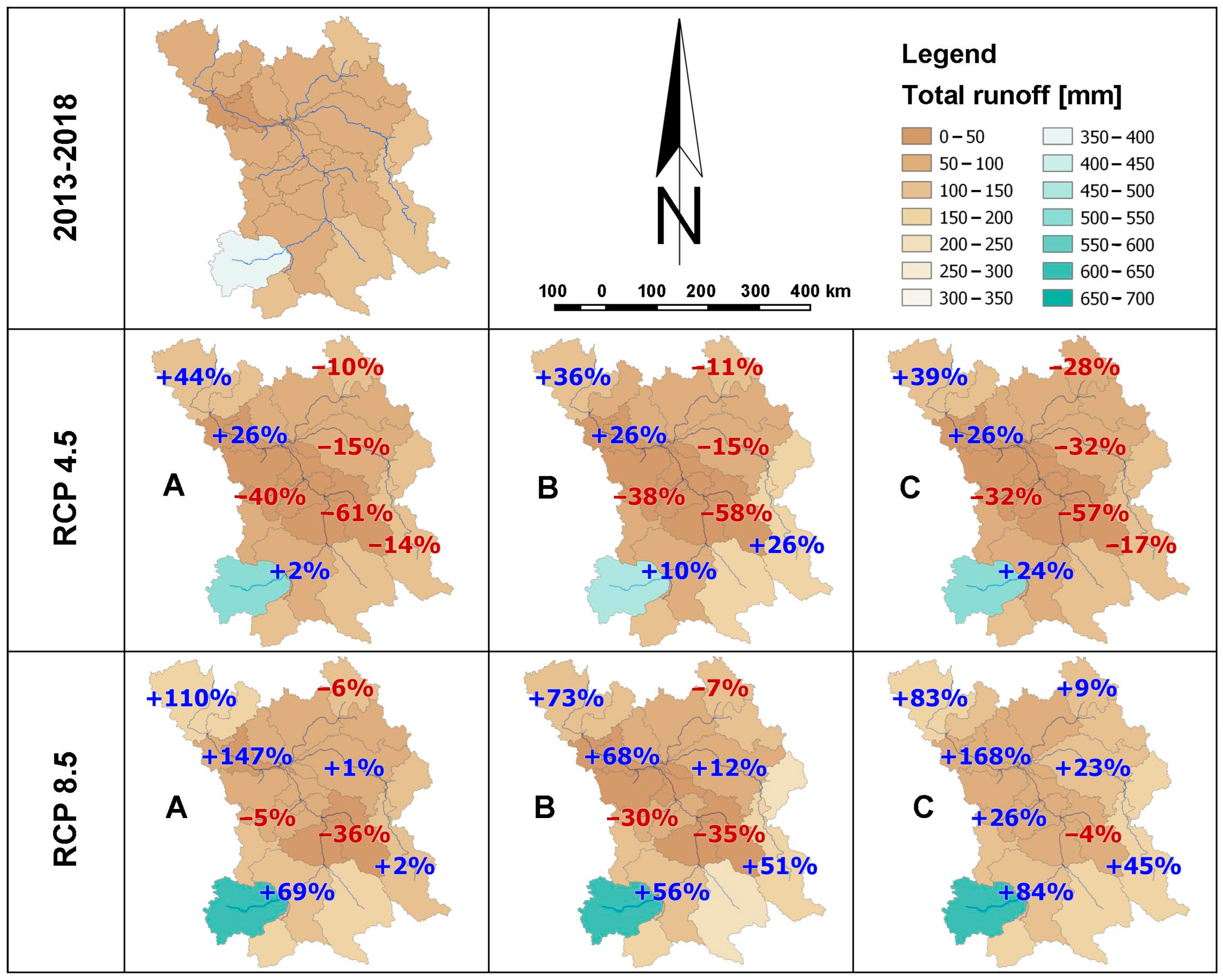
Annual mean total runoff totals over the 2013–2018 SWAT simulation period will be lower in most regions in the coming decades for most climate projections, with the exception of projection RCP 8.5.C (Figure 11). Larger annual mean total runoff totals can be found in the Northwest and South regions.

6. Discussion

The objective of this paper is to examine the hydrology of the Vistula catchment within the climate projections for 2020–2050, considering the climate change scenarios RCP 4.5 and RCP 8.5, and to evaluate it in light of the existing body of knowledge concerning research spanning both the European continent and smaller regional catchments.

The climate projection for Poland shows increased monthly precipitation values in winter and summer for the RCP 4.5 scenario for 2021–2030 compared to 2011–2020 [57]. In contrast, in spring, average monthly precipitation is lower than in 2011–2020. In the RCP 8.5 scenario for 2021–2030, average monthly precipitation changes slightly in most months compared to 2011–2020, while in autumn months, average monthly precipitation is higher in 2021–2030 [57]. In the article, all climate projections for 2021–2030 for the RCP 4.5 and RCP 8.5 scenarios are characterised by higher precipitation in winter (DJF) and summer (JJA) compared to 2013–2018. In autumn (SON), precipitation will be lower for most projections for 2021–2030. The same will be true for spring (MAM). For RCP 8.5.C projections for 2021–2030, most projections predict higher precipitation in winter, spring, summer, and autumn (Table 4).

The climate projection for the RCP 4.5 scenario for 2041–2050 shows increased monthly precipitation values in winter, summer, and autumn. In contrast, the spring months show lower average monthly precipitation compared to 2011–2020. For the RCP 8.5 scenario for 2041–2050, all months show increased average monthly precipitation compared to 2011–2020 [57]. In the paper, all climate projections for 2041–2050 for the RCP 4.5 scenario are characterised by higher average seasonal precipitation in summer (JJA) compared to 2013–2018. In autumn (SON), precipitation will be lower for RCP 4.5.A and RCP 4.5.B projections. In winter (DJA) and spring (MAM), precipitation will be higher for most projections. For RCP 8.5.A, RCP 8.5.B, RCP 8.5.C projections between 2041 and 2050, most projections predict higher precipitation in winter, spring, summer, and autumn (Table 4).

Changes in mean annual precipitation and total runoff were also considered in a publication on runoff in the Oder and Vistula catchments [20]. The publication shows that when comparing the 1971–2000 simulation period with the 2021–2050 period for RCP 4.5 and RCP 8.5 scenarios, there is an increase in mean annual precipitation and mean annual total runoff. In this paper, mean annual total runoff and mean annual precipitation tend to increase for most projections compared to the 2013–2018 simulation years.

The occurrence of drought in Poland has been an increasingly frequent and intense phenomenon in recent years, especially since 2006 [7]. It is a serious economic problem for the whole country. Drought causes large crop losses, reducing farmers’ income and thus increasing the price of food products [8]. The drought in 2015 had a very negative impact on agricultural crops. It occurred among all monitored crops [60]. The very hot and dry summer resulted in a hydrological drought in addition to heavy agricultural losses [61]. A partial water shortage also occurred in 2016 [62]. On the other hand, in 2017, no agricultural drought occurred in Poland in most reporting periods (9 out of 14 reports) [63]. Analysing 2018 from January to September, it can be concluded that it was a year characterised by high air temperatures (April, May, June, July, and August). In April and May, large differences were found in terms of precipitation. June was characterised by very low precipitation (except in the southern part of Poland). July, on the other hand, was characterised by high rainfall (except in the southern part of Poland). August was exceptionally warm this year, with varied precipitation [64]. The persistent precipitation deficiency from mid-April onwards, combined with high air temperatures and considerable sunshine, resulting in increased evaporation, caused droughts from April to September over large areas of Poland [37].

As per the National Oceanic and Atmospheric Administration (NOAA), 2017 ranked as the second-hottest year globally in recorded meteorological history (since 1880) [65]. Climate change will also affect Poland in the future. Analysis of climate scenarios for 2021–2050 shows that the growing season in Poland, defined by the number of days with an average daily air temperature higher than 5 °C in the 2021–2050 perspective, will be longer than in 1971–2000 by 16 days. The predicted higher temperature during the growing season would significantly accelerate the development of plants [57]. The trend in the annual average number of days with a mean temperature above 5 °C between 2020 and 2050 for most climate projections will increase, with the exception of the projection for scenario RCP 4.5.A (Figure 8).

Changes in the sum of mean annual precipitation in Poland between the control period 1971–2000 and the period 2021–2050 were compared for the RCP 4.5 scenario [66]. The publication shows that the sum of mean annual precipitation between the control period 1971–2000 and the period 2021–2050 will increase by 6.4%. For the Vistula basin, the sum of mean annual precipitation will increase between 2021 and 2050 for all climate projections compared to the simulation years 2013–2018.

In a publication on the Oder and Vistula catchments [19], the application of the SWAT model to simulate the water balance and natural flow of watercourses in the Vistula and Oder catchments from 1984 to 2013 is presented, followed by the results in the form of the concepts blue water flow, green water flow, and green water storage [67,68]. Blue water flow is the sum of ‘water yield’ and ‘deep aquifer recharge.’ Green water flow is the actual evapotranspiration, while green water storage is the soil water content [19]. Average results for the Vistula basin from 1984 to 2013 show blue water flow at 188 mm, green water flow at 521 mm, and green water retention at 211 mm. Results obtained for this article (2013–2018): blue water flow 234 mm, green water flow 402 mm, green water storage 171 mm. 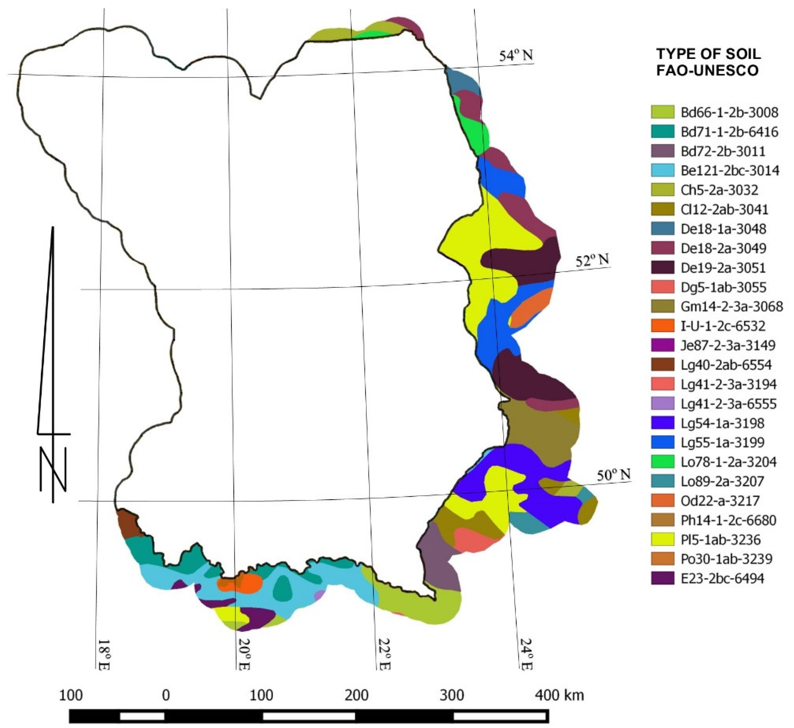The values obtained [19] were compared with the results of publications on the SWAT hydrological model for Europe [22] from 1973 to 2006. Blue water flow for Poland ranges from 50 to 200 mm, green water flow from 390 to 430 mm, and green water storage from 100 to 190 mm. The discrepancies in the results are probably due to the lower resolution of the HWSD 1: 1,000,000 and IUNG-PIB 1: 500,000 soil maps, which were introduced into the SWAT model in the article on the Vistula and Odra regions [19]. In this publication, the soil map IUNG-PIB 1: 100,000 was mainly used. While preparing the soil data, we took into account that the available water-holding capacity values are applicable to the soils in the Vistula River basin. These values were derived from a study conducted in 2013 by researchers from the Department of Soil Science, Erosion, and Soil Protection at IUNG-PIB in Puławy [69].

An examination of publications regarding the influence of climate change on the water resources of three Ukrainian catchments was conducted utilising the SWIM model [70]. One of the catchments studied is the Bug River. The study area of the Bug catchment included its part located in Ukraine, which is also included in the area of the present study [71]. Studies have shown an increase in precipitation, especially in spring and winter, and an increase in temperature under most climate change scenarios, which is also confirmed in this article.

Consistent findings regarding increased precipitation and temperature for climate change scenarios between 2071 and 2100 were achieved in studies of three Estonian catchments employing the SWAT model [72] and two catchments in Poland [10].

The study for the Neajlov River (southeastern part of Romania) with a catchment area of 3720 km² used output data from three GCMs (CNRM, MPR, and ICHEC) under two future climate projections (RCP 4.5 and RCP 8.5) in SWAT, which cover the periods 2021–2050 and 2071–2100 [73]. The projected changes in temperature and precipitation will be most noticeable during the growing season, leading to increased water stress. Different climate change scenarios, such as RCP 4.5 and RCP 8.5, exhibit diverse impacts on the hydrological cycle. In both short- and long-term perspectives, projected changes in temperature and precipitation will affect soil water content and streamflow, particularly in the lower watershed areas. For RCP 4.5, a moderate increase in SW is anticipated in the short term, but in the long term, a decline is expected, while RCP 8.5 indicates more significant reductions in both short- and long-term periods. This finding underscores the need to consider this diverse response to climate change when planning adaptive strategies related to water resources, with particular attention to lower watershed areas that appear more sensitive to these changes [73].

In a study conducted for the Manning River catchment in eastern Australia, hydrological responses to climate change were examined using the Xinanjiang (XAJ) model and downscaled climate data from 28 global climate models (GCMs) under RCP 8.5 scenarios [74].

The results show a slight decrease in annual precipitation and runoff between 2021 and 2060, followed by an increase between 2061 and 2100. While annual actual evapotranspiration is projected to increase slightly, soil moisture content is expected to decrease in the future. Changes in rainfall mainly affect future changes in seasonal and annual runoff, actual evapotranspiration, and soil moisture, with temperature changes playing a lesser role. The 28 GCM team predicts increased monthly and seasonal variability in water resources, characterised by higher values of high runoff and lower values of low runoff [74].

In a study conducted in the Gediz watershed in Turkey, downscaled general circulation model (GCM) data for monthly precipitation were utilised, employing representative concentration pathways (RCP). Projections were based on output data from 12 GCMs for the period 2015–2050. The findings indicate a significant decreasing trend in precipitation for the RCP 8.5 scenario, while it is less pronounced for the RCP 4.5 and RCP 6.0 scenarios [75]. This is an example of the impact of different climate change projection scenarios on the hydrological cycle.

The climate analysis for 1970–2004 reveals a statistically significant rise in total evapotranspiration throughout the growing season. Additionally, the years 2021–2030 and 2041–2050 exhibit an increase in potential evapotranspiration during the growing season (Table 7) [76].

The actual evapotranspiration, potential evapotranspiration, mean annual precipitation, and mean annual total runoff were also compared with the results of a publication on actual evapotranspiration in Europe [77]. Mean annual evapotranspiration, mean annual precipitation, and mean annual total outflow cover the years 2002–2014. For the Vistula basin, the mean annual actual evapotranspiration is in the range of 300–500 mm, the mean annual precipitation in the aforementioned publication is in the range of 500–700 mm, and the mean annual total outflow is in the range of 100–200 mm. The mean annual potential evapotranspiration covers the period 2002–2012 and is in the range of 650–750 mm. Similar results for potential evapotranspiration are included in a publication on the impact of climate change on Europe [78].

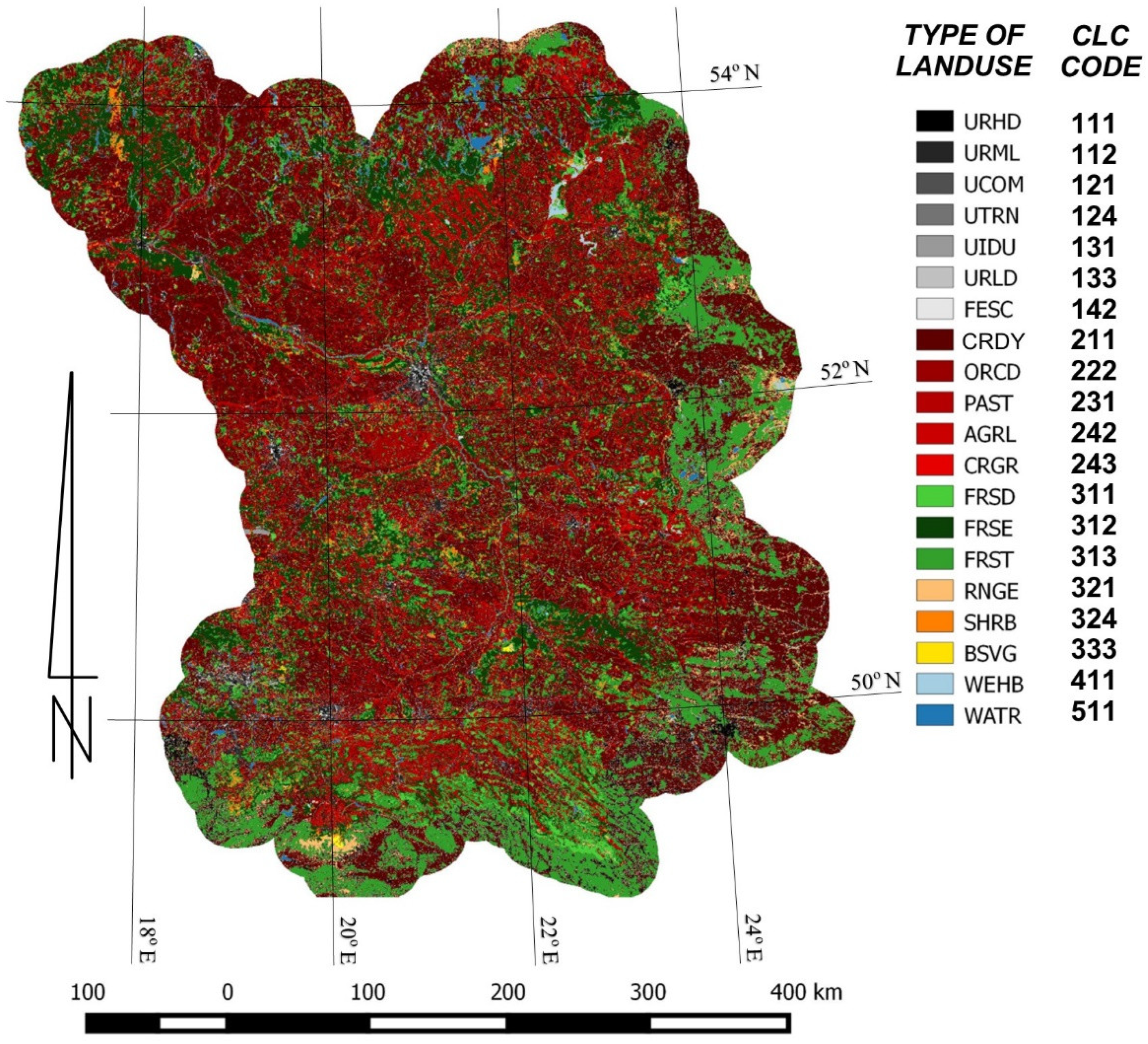
In conclusion, there are some differences in the results, but explaining these would require an extensive analysis of other potential factors influencing the spatial variability of the runoff response, such as land cover, soil, and hydrogeology. Such an analysis could be carried out in future studies.

7. Summary

Most climate change projections for the RCP 4.5 and RCP 8.5 scenarios show a trend of increasing temperature and precipitation in the coming decades. For most of the projections, the number of days with an average temperature above 5 °C will be higher, indicating that the growing season will become longer in the future. However, there are no clear results on how precipitation-free periods will develop in the future, as the number of days without precipitation varies from forecast to forecast.

For most of the projections analysed, the distribution of seasonal mean temperature in 2021–2030, 2031–2040, and 2041–2050, relative to the 2013–2018 period, indicates higher temperatures in the MAM season.

The average annual temperature for most climate projections for 2021–2030 will fall to as low as 8.7 °C (RCP 4.5.B) compared to the 2013–2018 simulation period (9.2 °C). In contrast, for all projections in 2031–2040 and 2041–2050, the average annual temperature will increase to as much as 10.3 °C (RCP 8.5.C).

A change in the seasonal distribution of rainfall is also to be expected. For most of the projections for 2021–2030, 2031–2040, and 2041–2050, precipitation is expected to increase in the JJA season compared to the 2013–2018 period. On an annual basis, precipitation is expected to be higher in the Northwest, South, and East regions by up to several tens of percent. In contrast, the amount of precipitation will decrease in the Central Vistula region by up to 17 percent for all projections in the RCP 4.5 scenario and for RCP 8.5.A and RCP 8.5.B projections in the RCP 4.5 scenario from 2041 to 2050. For most sub-catchments, increased annual precipitation is projected from 2041 to 2050 for climate projections RCP 8.5.C and RCP 8.5.C.

The average annual precipitation for all projections in 2021–2030, 2031–2040, and 2041–2050 will be higher by up to 22% (763 mm) (RCP 8.5.C for 2041–2050) compared to the 2013–2018 simulation years (624 mm). The trend of current evapotranspiration and potential evapotranspiration will differ between the 2020 and 2050 projections. The trend line of the average annual sum of potential evapotranspiration in projections RCP 8.5.A and RCP 8.5.B will decrease slightly in the coming decades. On the other hand, for the RCP 4.5.C and RCP 8.5.C projections and the RCP 4.5.B scenarios, the average annual sum of potential evapotranspiration increases in the coming decades.

The average annual actual evapotranspiration for all projections in 2021–2030, 2031–2040, and 2041–2050 will increase up to 467 mm (RCP 4.5.A—2021–2030) compared to the 2013–2018 simulation period of 401 mm.

The average annual potential evapotranspiration for all projections in 2021–2030, 2031–2040, and 2041–2050 will increase up to 755 mm (RCP 8.5.C—2031–2040) compared to the 2013–2018 simulation period—616 mm.

The trend of average annual evapotranspiration totals between 2020 and 2050 in all projections changes slightly.

In most climate projections, seasonal average evapotranspiration and potential evapotranspiration totals will be higher compared to the 2013–2018 model simulation period.

The average annual total runoff in all projections for the RCP 4.5 scenario will decrease between 2020 and 2050. On the other hand, in all projections for the RCP 8.5 scenario, the average annual total runoff will trend upward.

The average annual total runoff for most projections in the following decades (2021–2030, 2031–2040, and 2041–2050) will increase up to 159 mm (RCP 4.5.B—2021–2030) compared to the 2013–2018 simulation period—116 mm.

The average annual total runoff over the 2013–2018 simulation period will be lower in most regions in the coming decades for most climate projections, with the exception of RCP 8.5.A. A larger average annual total runoff can be found in the Northwest and South regions. All of the above changes in the individual components of the water balance may adversely affect crop vegetation in 2020–2050. The trend of increased temperatures and reduced precipitation may lead to long-term climate change as well as increased extreme events. Increased seasonal mean evapotranspiration and changes in soil water content may disrupt the vegetation of crops grown in Poland at every stage of growth, from sowing to harvest. The trend of an increase in average annual total runoff for the RCP 8.5 scenario and changes in the periods of the year when runoff will be higher may exacerbate erosion phenomena. Changes in the water balance between 2020 and 2050 will also depend on the particular Vistula catchment region.

This study contributes to a better understanding of the impact of climate change on hydrological processes at the watershed scale. Furthermore, the methodology applied in this research can be applied in other regions and consider additional factors such as land use and land cover changes to assess the influence of climate change on hydrological processes. It can provide support in formulating and implementing effective water resource management plans to minimise the impact of future climate changes on watershed-scale water resources.

References

1. Poskrobko, B.; Poskrobko, T.; Skiba, K. Ochrona Biosfery; Wydawnictwo Ekonomiczne: Warsaw, Poland, 2007. [Google Scholar]
2. Kowalik, P.; Scalenghe, R. Water Need of Energy Crops—One of the Environmental Problems of Poland. In Environmental Engineering III; CRC Press: Boca Raton, FL, USA, 2010; pp. 473–477. [Google Scholar]
3. Khatri, N.; Tyagi, S. Influences of natural and anthropogenic factors on surface and groundwater quality in rural and urban areas. Front. Life Sci. 2014, 8, 23–39. [Google Scholar] [CrossRef]
4. Główny Urząd Statystyczny. Zasoby Słodkiej Wody w Polsce—Raport 2020—Polska na Drodze Zrównoważonego Rozwoju; Główny Urząd Statystyczny: Warsaw, Poland, 2021. [Google Scholar]
5. Madej, P.; Konieczny, R.; Grela, J.; Korol, R. Stan i Wykorzystanie Zasobów wód Powierzchniowych Polski Monografia; Instytut Meteorologii i Gospodarki Wodnej, Warszawa: Kraków, Poland, 1996. [Google Scholar]
6. Kundzewicz, Z.W.; Kozyra, J. Ograniczanie wpływu zagrożeń klimatycznych w odniesieniu do rolnictwa i obszarów wiejskich. Pol. J. Agron. 2011, 7, 68–81. [Google Scholar]
7. Doroszewski, A.; Jóźwicki, T.; Wróblewska, E.; Kozyra, J. Susza Rolnicza w Polsce w Latach 1961–2010; Wydawnictwo IUNG PIB: Puławy, Poland, 2014. [Google Scholar]
8. Doroszewski, A.; Jadczyszyn, J.; Kozyra, J.; Pudełko, R.; Stuczyński, T.; Mizak, K.; Łopatka, A.; Koza, P.; Górski, T.; Wróblewska, E. Podstawy systemu monitoringu suszy rolniczej. Woda Sr. Obsz. Wiej. 2012, 12, 77–91. [Google Scholar]
9. Aydinalp, C.; Cresser, M. The Effects of Global Climate Change on Agriculture. Am. Eurasian J. Agric. Environ. Sci. 2008, 3, 672–676. [Google Scholar]
10. Marcinkowski, P.; Piniewski, M.; Kardel, I.; Szcześniak, M.; Benestad, R.; Srinivasan, R.; Ignar, S.; Okruszko, T. Effect of Climate Change on Hydrology, Sediment and Nutrient Losses in Two Lowland Catchments in Poland. Water 2017, 9, 156. [Google Scholar] [CrossRef]
11. Gudowicz, J. Modelowanie transportu materiału zawieszonego w dorzeczu Parsęty z uwzględnieniem zróżnicowanych rozdzielczości danych przestrzennych. Landf. Anal. 2015, 30, 57–64. [Google Scholar] [CrossRef]
12. Gudowicz, J.; Zwoliński, Z. Kształtowanie się odpływu rzecznego w dorzeczu Parsęty w świetle modelowania hydrologicznego = Shaping of river outflow in the Parsęta basin in the light of hydrological modelling. Przegląd Geogr. 2017, 89, 45–66. [Google Scholar] [CrossRef]
13. Gudowicz, J. Wpływ jakości danych przestrzennych na wyniki modelowania obiegu wody w dorzeczu Parsęty. Rocz. Geomatyki 2020, 14, 437–446. [Google Scholar]
14. Orlińska-Woźniak, P.; Szalińska, E.; Wilk, P. Do Land Use Changes Balance out Sediment Yields under Climate Change Predictions on the Sub-Basin Scale? The Carpathian Basin as an Example. Water 2020, 12, 1499. [Google Scholar] [CrossRef]
15. Brzozowski, J.; Miatkowski, Z.; Sliwinski, D.; Smarzynska, K.; Smietanka, M. Application of SWAT model to small agricultural catchment in Poland. J. Water Land Dev. 2011, 15, 157–166. [Google Scholar] [CrossRef]
16. Smarzyńska, K.; Miatkowski, Z. Calibration and validation of SWAT model for estimating water balance and nitrogen losses in a small agricultural watershed in central Poland. J. Water Land Dev. 2016, 29, 31–47. [Google Scholar] [CrossRef]
17. Miatkowski, Z.; Smarzyńska, K. Surface water resources of small agricultural watershed in the Kujawy region, central Poland. J. Water Land Dev. 2017, 33, 131–140. [Google Scholar] [CrossRef]
18. Ostojski, M.S.; Niedbala, J.; Orlinska-Wozniak, P.; Wilk, P.; Gębala, J. Soil and Water Assessment Tool Model Calibration Results for Different Catchment Sizes in Poland. J. Environ. Qual. 2014, 43, 132–144. [Google Scholar] [CrossRef] [PubMed]
19. Piniewski, M.; Szcześniak, M.; Kardel, I.; Berezowski, T.; Okruszko, T.; Srinivasan, R.; Schuler, D.V.; Kundzewicz, Z.W. Hydrological modelling of the Vistula and Odra river basins using SWAT. Hydrol. Sci. J. 2017, 62, 1266–1289. [Google Scholar] [CrossRef]
20. Piniewski, M.; Szcześniak, M.; Huang, S.; Kundzewicz, Z.W. Projections of runoff in the Vistula and the Odra river basins with the help of the SWAT model. Hydrol. Res. 2018, 49, 303–317. [Google Scholar] [CrossRef]
21. Piniewski, M.; Szcześniak, M.; Kardel, I. CHASE-PL—Future Hydrology Data Set: Projections of Water Balance and Streamflow for the Vistula and Odra Basins, Poland. Data 2017, 2, 14. [Google Scholar] [CrossRef]
22. Abbaspour, K.C.; Rouholahnejad, E.; Vaghefi, S.; Srinivasan, R.; Yang, H.; Kløve, B. A continental-scale hydrology and water quality model for Europe: Calibration and uncertainty of a high-resolution large-scale SWAT model. J. Hydrol. 2015, 524, 733–752. [Google Scholar] [CrossRef]
23. Dynowska, I.; Gilewska, S.; Kostrowicki, A.S.; Kozarski, J.; Paszyński, L. Geografia Polski Środowisko Przyrodnicze; Wydawnictwo Naukowe PWN SA, Warszawa: Warsaw, Poland, 1999. [Google Scholar]
24. Kubiak-Wójcicka, K. Flow Characteristics of the Vistula River at the Tczew Gauging Station in 1951–2010 Based on Flashiness Index. In Water Resources and Wetlands: 4th International Conference, Tulcea, Romania, 5–9 September 2018; Conference Proceedings; Gâştescu, P., Bretcan, P., Eds.; Romanian Limnogeographical Association: Târgovişte, Romania, 2018; pp. 119–129. [Google Scholar]
25. Kubiak-Wójcicka, K.; Bąk, B. Monitoring of meteorological and hydrological droughts in the Vistula basin (Poland). Environ. Monit. Assess. 2018, 190, 691. [Google Scholar] [CrossRef]
26. Tomczyl, A.M.; Bednorz, E. Atlas Klimatu Polski (1991–2020); Bogucki Wydawnictwo Naukowe: Poznań, Poland, 2022. [Google Scholar]
27. Arnold, J.; Kiniry, J.; Srinivasan, R.; Williams, J.; Haney, E.; Neitsch, S. Soil & Water Assessment Tool: Input/Output Documentation Version 2012; TR-439, 1–650; Texas Water Resources Institute: College Station, TX, USA, 2012. [Google Scholar]
28. QGIS. Quantum, GIS 3.10.13 Coruna; GIS Cloud: Zagreb, Croatia, 2020. [Google Scholar]
29. Winchell, M.; Srinivasan, R. SWAT Editor for SWAT 2012—Documentation; Blackland Research Center: Temple, TX, USA, 2012. [Google Scholar]
30. Abbaspour, K.C. SWAT-CUP 2012, SWAT Calibration and Uncertainty Programs—A User Manual; Eawag: Dübendorf, Switzerland, 2015. [Google Scholar]
31. CODGiK. Centralny Ośrodek Dokumentacji Geodezyjnej I Kartograficznej. Przegląd Geod. 2013, 69, 18–20. [Google Scholar]
32. MPHP. Komputerowa Mapa Podziału Hydrograficznego. 2017. Available online: https://danepubliczne.gov.pl/dataset?q=zlewnia&sort=metadata_modified+desc (accessed on 4 June 2018).
33. FAO/UNESCO. Digital Soil Map of the World F and AO of the UNV 3. 6 DSMW; Food and Agriculture Organization: Rome, Italy, 2003. [Google Scholar]
34. FAO—Unesco Soil Map of the World 1:5,000,000 Volume V Europe. Available online: https://www.fao.org/3/as354e/as354e.pdf (accessed on 15 July 2019).
35. SMGP. Szczegółowa Mapa Geologiczna Polski; Państwowy Instytut Geologiczny: Warszawa, Poland, 2006. [Google Scholar]
36. CLC. Corin Land Cover—CLC 2018; Główny Inspektorat Ochrony Środowiska: Warszawa, Poland, 2018. [Google Scholar]
37. IMGW. Instytut Meteorologii i Gospodarki Wodnej PIB. 2019. Available online: http://danepubliczne.imgw.pl/data/dane_pomiarowo_obserwacyjne/ (accessed on 3 March 2019).
38. USDA. United States Department of Agriculture. 1996. Available online: https://www.usda.gov/ (accessed on 1 December 2020).
39. Polskie Towarzystwo Gleboznawcze (PTG). Genetyczna klasyfikacja gleby Polski. Pol. Rocz. Glebozn. 1956, 7, 1–108. [Google Scholar]
40. Polskie Towarzystwo Gleboznawcze (PTG). Systematyka Gleb Polski. Rocz. Glebozn. 1989, 40, 132–133. [Google Scholar]
41. Polskie Towarzystwo Gleboznawcze (PTG). Classification of grain size in soils and mineral formations. Rocz. Glebozn. 2008, 60, 5–16. [Google Scholar]
42. Stępień, M.; Bodecka, E.; Gozdowski, D.; Wijata, M.; Groszyk, J.; Studnicki, M.; Sobczyński, G.; Rozbicki, J.; Samborski, S. Zgodność pomiędzy grupami granulometrycznymi określonymi według normy BN-78/9180-11 a grupami granulometrycznymi według PTG 2008 i klasami uziarnienia USDA. Soil Sci. Annu. 2018, 69, 223–233. [Google Scholar] [CrossRef]
43. Kabała, C.; Charzyński, P.; Chodorowski, J.; Drewnik, M.; Glina, B.; Greinert, A.; Hulisz, P.; Jankowski, M.; Jonczak, J.; Łabaz, B.; et al. Polish Soil Classification, 6th edition—Principles, classification scheme and correlations. Soil Sci. Annu. 2019, 70, 71–97. [Google Scholar] [CrossRef]
44. Batjes, N. IPCC Default Soil Classes Derived from the Harmonized World Soil Data Base (Version 1.1); Wageningen University & Research: Wageningen, The Netherlands, 2010. [Google Scholar]
45. Badora, D.; Wawer, R.; Nierobca, A.; Krol-Badziak, A.; Kozyra, J.; Jurga, B.; Nowocien, E. Modelling the Hydrology of an Upland Catchment of Bystra River in 2050 Climate Using RCP 4.5 and RCP 8.5 Emission Scenario Forecasts. Agriculture 2022, 12, 403. [Google Scholar] [CrossRef]
46. Essenfelder, A.H. SWAT Weather Database: A Quick Guide Version: V.0.18.03. 2018. Available online: https://doi:10.13140/RG.2.1.4329.1927 (accessed on 3 March 2020).
47. KPOŚK. Krajowy Program Oczyszczania Ścieków Komunalnych. 2017. Available online: https://www.kzgw.gov.pl/index.php/pl/materialy-informacyjne/programy/krajowy-program-oczyszczania-sciekow-komunalnych (accessed on 3 March 2020).
48. Abbaspour, K.C. SWAT-CUP Tutorial (2): Introduction to SWAT-CUP Program; Parameter Estimator (SPE), Program 2w2e GmbH. 2020. Available online: https://www.youtube.com/watch?v=nNsDPhOI7cc (accessed on 15 June 2023).
49. Arnold, J.G.; Moriasi, D.N.; Gassman, P.W.; Abbaspour, K.C.; White, M.J.; Srinivasan, R.; Santhi, C.; Harmel, R.D.; van Griensven, A.; Van Liew, M.W.; et al. SWAT: Model Use, Calibration, and Validation. Trans. ASABE 2012, 55, 1491–1508. [Google Scholar] [CrossRef]
50. Kouchi, D.H.; Esmaili, K.; Faridhosseini, A.; Sanaeinejad, S.H.; Khalili, D.; Abbaspour, K.C. Sensitivity of Calibrated Parameters and Water Resource Estimates on Different Objective Functions and Optimization Algorithms. Water 2017, 9, 384. [Google Scholar] [CrossRef]
51. Thomson, A.M.; Calvin, K.V.; Smith, S.J.; Kyle, G.P.; Volke, A.; Patel, P.; Delgado-Arias, S.; Bond-Lamberty, B.; Wise, M.A.; Clarke, L.E.; et al. RCP4.5: A pathway for stabilization of radiative forcing by 2100. Clim. Chang. 2011, 109, 77–94. [Google Scholar] [CrossRef]
52. Hennemuth, T.I.; Jacob, D.; Keup-Thiel, E. Guidance for EURO-CORDEX Climate Projections Data Use. Version1 0-201708. 2017. Available online: https://www.euro-cordex.net/imperia/md/content/csc/cordex/euro-cordex-guidelines-version1.0-2017.08.pdf (accessed on 13 January 2020).
53. Jacob, D.; Petersen, J.; Eggert, B.; Alias, A.; Christensen, O.B.; Bouwer, L.M.; Braun, A.; Colette, A.; Déqué, M.; Georgievski, G.; et al. EURO-CORDEX: New high-resolution climate change projections for European impact research. Reg. Environ. Chang. 2014, 14, 563–578. [Google Scholar] [CrossRef]
54. Yang, W.; Andréasson, J.; Graham, L.P.; Olsson, J.; Rosberg, J.; Wetterhall, F. Distribution-based scaling to improve usability of regional climate model projections for hydrological climate change impacts studies. Hydrol. Res. 2010, 41, 211–229. [Google Scholar] [CrossRef]
55. Landelius, T.; Dahlgren, P.; Gollvik, S.; Jansson, A.; Olsson, E. A high-resolution regional reanalysis for Europe. Part 2: 2D analysis of surface temperature, precipitation and wind. Q. J. R. Meteorol. Soc. 2016, 142, 2132–2142. [Google Scholar] [CrossRef]
56. Schulzweida, U.; Kornblueh, L.; Quast, R. CDO User’s Guide. Climate Data Operators Version 1.5.9. 2012. Available online: http://www.idris.fr/media/ada/cdo.pdf (accessed on 3 March 2022).
57. KLIMADA. 2.0 KLIMADA 2.0—Baza Wiedzy o Zmianach Klimatu, Scenariusze Zmian Klimatu. 2019. Available online: https://klimada2.ios.gov.pl (accessed on 5 February 2022).
58. PIK. Potsdam Institute for Climate Impact. 2012. Available online: https://www.pik-potsdam.de/~mmalte/rcps/ (accessed on 10 August 2022).
59. Meinshausen, M.; Smith, S.J.; Calvin, K.; Daniel, J.S.; Kainuma, M.L.; Lamarque, J.F.; Matsumoto, K.; Montzka, S.A.; Raper, S.C.; Riahi, K.; et al. The RCP greenhouse gas concentrations and their extensions from 1765 to 2300. Clim. Chang. 2011, 109, 213–241. [Google Scholar] [CrossRef]
60. Doroszewski, A. Agricultural Drought in Poland in 2015 Conference 24 February 2016 Warsaw. Warsaw. 2016. Available online: http://gwppl.org/data/uploads/prezentacje/4.%20Susza%20rolnicza_ADoroszewski.pdf (accessed on 12 February 2023).
61. IUNG-PIB. 2015—Message of Drought Occurrence in Poland; IUNG-PIB: Puławy, Poland, 2015. [Google Scholar]
62. IUNG-PIB. 2016—Message of Drought Occurrence in Poland; IUNG-PIB: Puławy, Poland, 2016. [Google Scholar]
63. IUNG-PIB. 2017—Message of Drought Occurrence in Poland; IUNG-PIB: Puławy, Poland, 2017. [Google Scholar]
64. IUNG-PIB. 2018—Drought Occurrence Announcement in Poland; IUNG-PIB: Puławy, Poland, 2018. [Google Scholar]
65. NOAA. National Oceanic and Atmospheric Administration, Global Summary Information—January 2018. 2018. Available online: https://www.ncdc.noaa.gov/sotc/global/201713 (accessed on 15 June 2021).
66. Mezghani, A.; Dobler, A.; Haugen, J.E.; Benestad, R.E.; Parding, K.M.; Piniewski, M.; Kardel, I.; Kundzewicz, Z.W. CHASE-PL Climate Projection dataset over Poland–bias adjustment of EURO-CORDEX simulations. Earth Syst. Sci. Data 2017, 9, 905–925. [Google Scholar] [CrossRef]
67. Falkenmark, M.; Rockström, J. The New Blue and Green Water Paradigm: Breaking New Ground for Water Resources Planning and Management. J. Water Resour. Plan. Manag. 2006, 132, 129–132. [Google Scholar] [CrossRef]
68. Schuol, J.; Abbaspour, K.C.; Yang, H.; Srinivasan, R.; Zehnder, A.J.B. Modeling blue and green water availability in Africa. Water Resour. Res. 2008, 44, 212–221. [Google Scholar] [CrossRef]
69. IUNG-PIB. Ocena Retencji Wody w Glebie i Zagrożenia Suszą w Oparciu o Bilans Wodny dla Obszaru Województwa Dolnośląskiego; IUNG-PIB: Puławy, Poland, 2013. [Google Scholar]
70. Krysanova, V.; Wechsung, F.; Arnold, J.; Srinivasan, R.; Williams, J. PIK Report Nr. 69 “SWIM (Soil and Water Integrated Model), User Manual”; Potsdam Institute for Climate Impact Research: Potsdam, Germany, 2000. [Google Scholar]
71. Didovets, I.; Lobanova, A.; Bronstert, A.; Snizhko, S.; Maule, C.F.; Krysanova, V. Assessment of Climate Change Impacts on Water Resources in Three Representative Ukrainian Catchments Using Eco-Hydrological Modelling. Water 2017, 9, 204. [Google Scholar] [CrossRef]
72. Tamm, O.; Luhamaa, A.; Tamm, T. Modeling future changes in the North-Estonian hydropower production by using SWAT. Hydrol. Res. 2015, 47, 835–846. [Google Scholar] [CrossRef]
73. Danielescu, S.; Adamescu, M.C.; Cheval, S.; Dumitrescu, A.; Cazacu, C.; Borcan, M.; Postolache, C. Climate Change Impacts on Hydrological Processes in a South-Eastern European Catchment. Water 2022, 14, 2325. [Google Scholar] [CrossRef]
74. Fengyun, Z. The effects of no-tillage practice on soil physical properties. Afr. J. Biotechnol. 2011, 10, 17645–17650. [Google Scholar] [CrossRef]
75. Okkan, U.; Kirdemir, U. Downscaling of monthly precipitation using CMIP5 climate models operated under RCPs. Meteorol. Appl. 2016, 23, 514–528. [Google Scholar] [CrossRef]
76. Łabędzki, L.; Bąk, B.; Kanecka-Geszke, E. Wielkość i zmienność ewapotranspiracji wskaźnikowej według Penmana-Monteitha w okresie wegetacyjnym w latach 1970–2004 w wybranych rejonach Polski. Woda Sr. Obsz. Wiej. 2012, 2, 159–170. [Google Scholar]
77. Stisen, S.; Soltani, M.; Mendiguren, G.; Langkilde, H.; Garcia, M.; Koch, J. Spatial Patterns in Actual Evapotranspiration Climatologies for Europe. Remote. Sens. 2021, 13, 2410. [Google Scholar] [CrossRef]
78. Teuling, A.J.; de Badts, E.A.G.; Jansen, F.A.; Fuchs, R.; Buitink, J.; van Dijke, A.J.H.; Sterling, S.M. Climate change, reforestation/afforestation, and urbanization impacts on evapotranspiration and streamflow in Europe. Hydrol. Earth Syst. Sci. 2019, 23, 3631–3652. [Google Scholar] [CrossRef]
Figure 1. The Vistula River basin, including the primary Vistula tributaries and their respective catchment areas, was delineated (own study).
Water 15 04168 g001
Figure 2. Distribution of soil types entered into the SWAT model with a breakdown by FAO-UNESCO soil types for areas outside Poland (own study).
Water 15 04168 g002
Figure 3. Distribution of land cover types of the Vistula River basin (own study).
Water 15 04168 g003
Figure 4. A total of 95 ppu plot and observed stream flow during calibration and validation (own study).
Water 15 04168 g004
Figure 5. Annual precipitation and annual temperature in the Vistula catchment from 2000 to 2050 for individual climate projections in the RCP 4.5 and RCP 8.5 scenarios with trend lines (own study).
Water 15 04168 g005
Figure 6. The annual sum of rainless days and the annual sum of days with temperatures exceeding 5 °C in the Vistula River basin for the years 2020–2050 for each climate projection in the RCP 4.5 and RCP 8.5 scenarios (own study).
Water 15 04168 g006
Figure 7. Annual sum of rain–free days in the Vistula River basin in 2021–2050 and the periods 2021–2030, 2031–2040, and 2041–2050 for individual climate projections in the RCP 4.5 and RCP 8.5 scenarios (own study).
Water 15 04168 g007
Figure 8. Average annual total runoff in the Vistula River basin from 2020 to 2050 for specific climate projections in the RCP 4.5 and RCP 8.5 scenarios, including trend lines (own study).
Water 15 04168 g008
Figure 9. Average annual actual and potential evapotranspiration in the Vistula catchment from 2020 to 2050 for specific climate projections in the RCP 4.5 and RCP 8.5 scenarios, including trend lines (own study).
Water 15 04168 g009
Figure 10. Comparing the mean precipitation across 23 sub-catchments during the SWAT simulation periods of 2013–2018 and 2040–2050, considering the various climate projections within the RCP 4.5 and RCP 8.5 scenarios, where (A, B, C) represent climate models (own study).
Water 15 04168 g010
Figure 11. Comparing the mean total runoff across 23 sub-catchments during the SWAT simulation periods of 2013–2018 and 2040–2050, considering the various climate projections within the RCP 4.5 and RCP 8.5 scenarios, where (A, B, C) represent climate models (own study).
Water 15 04168 g011