Fragility Analysis for Water-Retaining Structures Resting on Spatially Random Soil

Abstract

The maintenance of water-retaining structures involves evaluating their performance against current and future operating water levels. Fragility curves are commonly used for this purpose, as they indicate the conditional probability of failure for various load conditions and accurately characterize a structure’s performance. Monte Carlo simulation (MCS) can be used to determine the fragility curve of water-retaining structures by calculating the probability of failure as the water level changes. However, performing repetitive MCS involves extensive calculations, thus making it inefficient for practical applications. Therefore, it is essential to develop efficient methods that require a minimum number of MCS runs to estimate the fragility curve. This study proposed two methods to estimate the fragility curves of water-retaining structures, thereby allowing for the assessment of failure probabilities related to important quantities such as the steady-state seepage rate, exit gradient, and uplift force, which make them suitable for practical applications. The fragility curves obtained using the proposed methods are valuable for risk assessment, design, and decision-making purposes, as they offer information to evaluate the performance of the water-retaining structure under various water level conditions.

1. Introduction

Due to recent climate change, there have been extreme floods that have exceeded the design criteria for water-retaining structures, thereby threatening safety. As a result, there has been a demand for developing technologies that can cope with such situations.

Effective asset management of flood defense infrastructure, such as dams, barrages, and embankments, necessitates a thorough evaluation of their performance against expected loads [1,2,3]. Fragility curves are frequently utilized for this purpose, as they represent the conditional probability of failure for various load conditions and can accurately characterize the performance of a structure [4,5]. Fragility curves have been extensively utilized in earthquake engineering to evaluate the performance of structures against maximum ground accelerations. Compared to point estimates, fragility curves provide a broader range of information about a structure’s reliability by offering continuous reliability information in the form of a curve or function [6,7]. Consequently, their application has been gaining increasing momentum in the field of risk assessment for various damage states of geotechnical structures, such as slopes, dams, and embankments (e.g., [1,5,7,8,9,10,11]). To evaluate the reliability of a levee within a probabilistic framework, fragility curves are employed for specific mechanisms as functions of conditioning loads, such as water level or water discharge [8,12,13,14,15].

The probabilistic analysis method is useful for evaluating the reliability and fragility of hydraulic structures because it can quantitatively consider the uncertainty and spatial variability of soil hydraulic conductivity in the analysis and design of seepage stability. Several researchers have conducted studies on probabilistic seepage analysis, which considered the spatial variability of soil properties [16,17,18,19,20,21,22,23,24,25,26]. Concerning seepage flow underneath a retaining structure, Griffiths and Fenton [27,28] considered the effect of spatial variability of hydraulic conductivity by combining the finite element method with the random field theory. Hekmatzadeh et al. [23] investigated the influence of uncertainty in the soil properties, earthquake coefficients, and sediment characteristics in the stability of a diversion dam against piping and sliding. Johari and Heydari [24] developed a method for reliability analysis of the steady state seepage using stochastic the Scaled Boundary Finite-Element Method to consider the spatial variability of the permeability. Robbins et al. [29] presented an application of the Random Finite Element Method (RFEM) to the simulation of backward erosion piping in order to quantitatively assess how spatial variability in soil properties influences pipe progression.

Within the framework of the random field theory, the hydraulic conductivity is expressed by a large number of random variables to represent the spatial variability. Therefore, the application of probabilistic analysis techniques such as the First-Order Reliability Method (FORM), the First-Order Second-Moment (FOSM) method, and more advanced techniques including artificial neural network and genetic algorithm for seepage analysis has not been reported. As a result, Monte Carlo simulation (MCS) has been exclusively employed for all probabilistic seepage analyses that consider the spatial variability of the hydraulic conductivity. Cho [30] proposed a procedure for determining the fragility curve from repetitive MCS and developed the fragility curve of the water-retaining structure depending on the location of the cutoff wall installed for seepage control. However, performing repetitive MCS requires extensive calculations, which makes it inefficient for practical applications. Therefore, developing efficient methods that require a minimum number of MCS runs to estimate the fragility curve is essential. This study proposed such methods to develop fragility curves for water-retaining structures founded on spatially random soil, making them suitable for practical applications. The failure probabilities needed for establishing the fragility curves rely on analyses utilizing stochastic seepage analysis. This approach considers the spatial variability of soil permeability, as outlined by Cho [31].

2. Methodology

2.1. Probabilistic Seepage Analysis

Assuming that water is incompressible, the differential equation expressing the two-dimensional steady-state flow through the soil is obtained from the continuity equation and Darcy’s law, as follows:

$$\frac{\partial }{\partial x}\left(k_x\frac{\partial h}{\partial x}\right)+\frac{\partial }{\partial y}\left(k_y\frac{\partial h}{\partial y}\right)=0,$$

(1)

where $h$ is the total head, and $k_x$ and $k_y$ are the hydraulic conductivity in the $x$ and $y$ directions, respectively.

In this study, the finite element method (FEM) was used for a two-dimensional steady-state seepage analysis that estimated the total head at nodes across the solution domain.

After discretization of Equation (1) in space with the Galerkin weighted residual method, a set of finite element equations can be obtained as:

$${\mathit{K}}_c\mathsf{\Phi }=\mathit{Q},$$

(2)

where ${\mathit{K}}_c$ is the global conductivity matrix, $\mathsf{\Phi }$ is the vector of nodal hydraulic head values, and $\mathit{Q}$ is the vector of nodal flow rates.

The global conductivity matrix ${\mathit{K}}_c$ is an assembly of the element conductivity matrices of the entire seepage domain. The element conductivity matrix is given as:

$${\mathit{k}}_c={\int }_{v_e}^{}{\left[\mathit{B}\right]}^T\left[\mathit{k}\right]\left[\mathit{B}\right]dv,$$

(3)

where $v_e$ is the domain of the element, $\left[\mathit{B}\right]$ is derived from the shape function, and $\left[\mathit{k}\right]$ is defined as:

$$\left[\mathit{k}\right]=\left[\begin{array}{cc}{k}_x& 0\\ 0& k_y\end{array}\right].$$

(4)

Additional seepage-related quantities, such as exit gradients, seepage rates, and uplift forces, were calculated based on the nodal head values. The exit gradient represented the rate of head change at the exit point immediately downstream of the water-retaining structure. The seepage rate was defined as the quantity of water that passed through the soil foundation per unit time.

Soil is a material that exhibits spatial variability, even in a homogeneous layer, due to depositional conditions and differing loading histories. This spatial variability is a major contributor to soil uncertainty [32]. The spatial variability of soil properties can be explained by the correlation structure within the theoretical framework of the random field model [33]. The autocorrelation distance is used to indicate the spatial extent over which the soil properties display a strong correlation.

A Gaussian random field is defined completely by the mean, variance, and autocorrelation function. In this study, an exponential autocorrelation function was used, and different autocorrelation distances in the vertical and horizontal directions were used as follows:

$$\rho \left(x,y\right)=\mathrm{e}\mathrm{x}\mathrm{p}\left(-\frac{\left|x-x^{\prime }\right|}{l_h}-\frac{\left|y-y^{\prime }\right|}{l_v}\right),$$

(5)

where $l_h$ and $l_v$ are the autocorrelation distances in the horizontal and vertical directions, respectively.

In this study, the RFEM was utilized to incorporate the soil spatial variability represented as random fields. The RFEM conducts multiple finite element analyses, with each analysis originating from a realization of the soil properties treated as a multidimensional random field [34]. The hydraulic conductivity, which is a soil characteristic related to seepage, should be modeled as a random field to represent spatial variability. Since the FEM utilized for seepage analysis has discontinuous characteristics, the random field of the hydraulic conductivity must be expressed with a finite number of random variables. This process is called the discretization of the random field. In this study, the Karhunen-Loève expansion method was used to discretize the two-dimensional random field of the hydraulic conductivity. Cho [31] provided a comprehensive procedure for the discretization of random fields.

The problem of probabilistic seepage analysis is formulated as a vector of random variables $\mathit{X}$ representing the seepage characteristics of the soil. The limit state function $g\left(\mathit{X}\right)$ defining the boundary between the safe state and failure state in the design variable space is determined by these random variables [31]. Subsequently, the failure probability is expressed as a multidimensional integral equation performed on the failure region:

$$P_f=P\left[g\left(\mathit{X}\right)\le 0\right]={\int }_{g\left(\mathit{X}\right)\le 0}^{}{f}_{\mathit{X}}\left(\mathit{X}\right)d\mathit{X},$$

(6)

where $f_{\mathit{X}}\left(\mathit{X}\right)$ represents the joint probability density function, and the integral is carried out over the failure domain. Failure does not necessarily imply the complete collapse of a structure, but rather a state that fails to meet the required performance criteria. Thus, the probability of failure is determined by calculating the probability of exceeding a given limit state. In an MCS, a series of random fields that match the probability distribution and correlation structure of the hydraulic conductivity is generated, and the limit state function for each generated random field is calculated. By repeating this process a sufficient number of times, the failure probability can be estimated accurately.

In the seepage problem, the limit state function that defines failure according to various failure modes related to piping, uplift force, and seepage rate can be defined in the following manner:

$$g\left(\mathit{X}\right)=s_{crit}-s\left(\mathit{X}\right),$$

(7)

where $s_{crit}$ is a critical value that causes failure for each failure mode, and $s\left(\mathit{X}\right)$ is a response value calculated by seepage analysis. That is, the limit state functions for piping, uplift force, and seepage rate are defined as follows:

$$g\left(\mathit{X}\right)=i_{crit}-i_e\left(\mathit{X}\right)\mathrm{f}\mathrm{o}\mathrm{r}\mathrm{p}\mathrm{i}\mathrm{p}\mathrm{i}\mathrm{n}\mathrm{g},$$

(7a)

$$g\left(\mathit{X}\right)=F_{cr}-F\left(\mathit{X}\right)\mathrm{f}\mathrm{o}\mathrm{r}\mathrm{u}\mathrm{p}\mathrm{l}\mathrm{i}\mathrm{f}\mathrm{t}\mathrm{f}\mathrm{o}\mathrm{r}\mathrm{c}\mathrm{e},$$

(7b)

$$g\left(\mathit{X}\right)=Q_{cr}-Q\left(\mathit{X}\right)\mathrm{f}\mathrm{o}\mathrm{r}\mathrm{s}\mathrm{e}\mathrm{e}\mathrm{p}\mathrm{a}\mathrm{g}\mathrm{e}\mathrm{r}\mathrm{a}\mathrm{t}\mathrm{e},$$

(7c)

where $i_{crit}$ is the critical hydraulic gradient, $F_{cr}$ is the critical uplift force, $Q_{cr}$ is the critical seepage rate, $i_e\left(\mathit{X}\right)$ is the exit hydraulic gradient, $F\left(\mathit{X}\right)$ is the uplift force, and $Q\left(\mathit{X}\right)$ is the seepage rate calculated by seepage analysis.

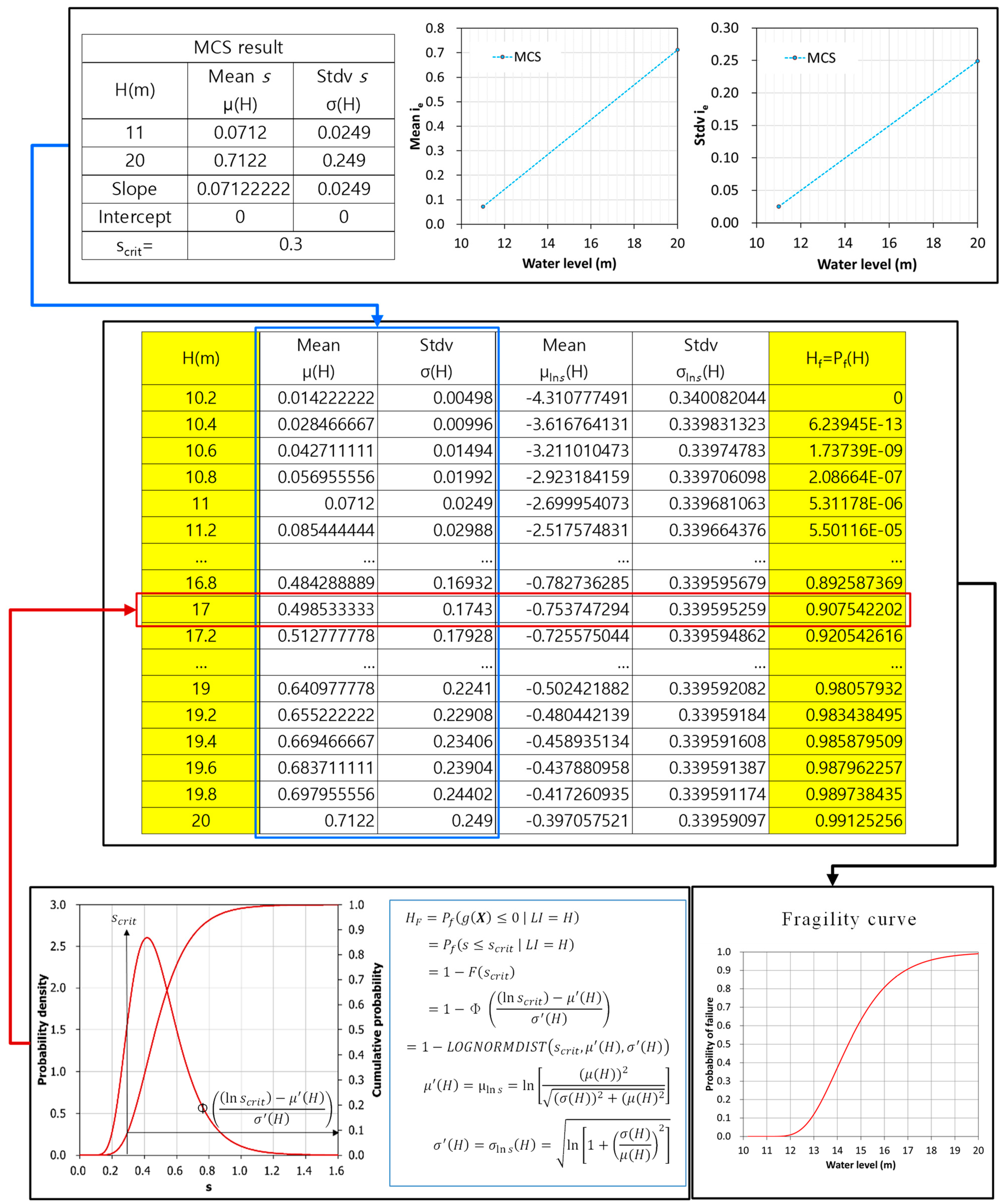
2.2. Fragility Curve

Fragility curves can be developed using various methods, including field observations of damage, structural analyses, and expert judgment [35]. In this study, analytical fragility curves were derived from steady-state seepage analysis. The fragility of a structure at a given load intensity was obtained from the results of MCS. Since the main load variable that governs the stability of water-retaining structures is the hydraulic head difference between the upstream and downstream sides of the structure that causes seepage, fragility curves were developed according to the water level upstream of the structure $H$.

$$P_f\left(H\right)=P\left(g\right(\mathit{X})\le \left.0\right|LI=H),$$

(8)

Equation (8) represents the conditional cumulative probability of a given loading condition over a range. The fragility curve represents the resistance of a water-retaining structure to a water level, but it does not account for the probability of a specific water level occurrence. Therefore, to calculate the final failure probability, the prepared fragility curve must be combined with the probability model for the water level [8].

In this study, two methods were proposed to develop fragility curves for water-retaining structures by reducing the number of time-consuming and computationally intensive MCS operations.

2.2.1. Method A

Once the parameters of the probability distribution function (PDF) for any two water levels are estimated, the parameters of $s$ at any other water level can be easily calculated using linear equations without requiring any additional MCS. If the parameters of the PDF of $s$ for a given water level are known, the failure probability $P_f$ can be calculated. By repeating this process and increasing the water level $H$, a fragility curve can be created. The fragility curve obtained using Method A is piecewise linear, but $P_f$ can be calculated by incrementing the water level to the desired level of precision, allowing for a smooth fragility curve to be easily created. Figure 1 shows a schematic representation of the fragility curve creation procedure using Method A.

A random variable $s$ is completely described if its probability distribution is specified. The parameters of the distribution are often derived as functions of the measures of central tendency and variability, or they may be the parameters themselves. The most common measures of central tendency and variability are the mean and the standard deviation, respectively [34].

The appropriate PDF of the exit hydraulic gradient, uplift force, and seepage rate obtained from the MCS results for seepage beneath a water-retaining structure can be selected from probability distribution fitting. Then the failure probability is calculated as follows:

$$P_f=P\left(s_{crit}\le s\right)=1-CDF\left(s_{crit}\right),$$

(9)

where $CDF\left(·\right)$ is the cumulative distribution function (CDF) of the selected PDF.

Spreadsheet software Excel provides cumulative probability distribution functions for various probability distributions, so Equation (9) can be easily calculated.

For explanatory purposes, assume that the random variable $s$ follows a lognormal distribution. When a continuous random variable $s$ with a mean of $\mu$ and a standard deviation of $\sigma$ follows a lognormal distribution where $0\le s\le +\mathrm{\infty }$, $\ln s$ follows a normal distribution with a mean of ${\mu }^{\prime }=\ln \left[\frac{{\mu }^2}{\sqrt{{\sigma }^2+{\mu }^2}}\right]$ and a standard deviation of ${\sigma }^{\prime }=\sqrt{\ln \left[1+{\left(\frac{\sigma }{\mu }\right)}^2\right]}$. The CDF is expressed as:

$$CDF\left(s\right)=\mathsf{\Phi }\left(\frac{\left(\ln s\right)-{\mu }^{\prime }}{{\sigma }^{\prime }}\right),$$

(10)

where Φ is the standard normal CDF.

As shown in Figure 1, Equation (9) can be easily computed using the LOGNORMDIST function in Excel. When the water level $H$ changes, the mean $\mu$ and the standard deviation $\sigma$ of the random variable $s$ change.

In the case of the flow rate, a normalized flow rate $\overline{Q}$ is defined for a given total head difference between the upstream and downstream sides, $∆H_1$:

$$\overline{Q}=\frac{Q(∆H_1)}{{\mu }_k{∆H}_1},$$

(11)

where ${\mu }_k$ is the mean hydraulic conductivity.

Since $\overline{Q}$ is equivalent to the “shape factor” of the problem, namely the ratio of the number of flow channels divided by the number of equipotential drops (n_f/n_d) that would be observed in a carefully drawn flow net [28,34], $\overline{Q}$ is determined regardless of $∆H$.

Then, the flow rate through the soil at any $∆H$ is obtained from Equation (11) as:

$$Q(∆H)={\mu }_k∆H\overline{Q},$$

(12)

which will have the same distribution as $\overline{Q}$ except with mean and standard deviation:

$${\mu }_Q(∆H)={\mu }_k∆H{\mu }_{\overline{Q}},$$

(13)

$${\sigma }_Q(∆H)={\mu }_k∆H{\sigma }_{\overline{Q}},$$

(14)

For the uplift force on the base of the dam, $F$, a nondimensional uplift force $\overline{F}$ is defined as:

$$\overline{F}=\frac{F(∆H_1)}{{\gamma }_w{∆H}_{1}L},$$

(15)

where ${\gamma }_w$ is the unit weight of water, $L$ is the length of the base of the structure.

Similarly, the distribution of $F(∆H)$ is the same as the distribution of $\overline{F}$ except with mean and standard deviation:

$${\mu }_F(∆H)=L{\gamma }_w∆H{\mu }_{\overline{F}},$$

(16)

$${\sigma }_F(∆H)=L{\gamma }_w∆H{\sigma }_{\overline{F}},$$

(17)

The exit gradient $i_e$ is defined as the first derivative of the total head with respect to length at the exit points. Therefore, the value of $i_e(∆H)$ is proportional to the head difference $H$ as:

$${\mu }_{i_e}(∆H)=(\frac{∆H}{{∆H}_1}){\mu }_{\overline{i_e}},$$

(18)

$${\sigma }_{i_e}(∆H)=(\frac{∆H}{{∆H}_1}){\sigma }_{\overline{i_e}},$$

(19)

where ${\mu }_{\overline{i_e}}$ and ${\sigma }_{\overline{i_e}}$ are the mean and standard deviation of exit gradient for ${∆H}_1$, respectively.

Once the mean and standard deviation of seepage output, the parameters of the PDF, are evaluated for one or two water levels from the MCS, the probability distribution is specified. The mean and standard deviation of random variable $s$, which represents the seepage behavior through the soil beneath a water-retaining structure, are directly proportional to the water head difference between the upstream and downstream faces (Equations (13), (14), (16)–(19)).

2.2.2. Method B

The lognormal CDF is the most common form of a seismic fragility function, although it is not universal [6]. In this study, fragility curves were created for a water-retaining structure by assuming a lognormal CDF. The equation for the lognormal CDF is as follows [11,36]:

$$P_f\left(H\right)=P(s_{crit}\le s\left|LI\right.=H)=\mathsf{\Phi }\left(\frac{\ln (H/\theta )}{\beta }\right),$$

(20)

where $P(·)$ represents the probability that a water level with $LI=H$ will cause the structure to fail. $\theta$ is the median of the fragility function (i.e., the water level with 50% probability of failure), and $\beta$ is the standard deviation of ln (LI). Equation (20) implies that the LI values of water levels causing failure of a given water-retaining structure are lognormally distributed. To calibrate Equation (20) for a given water-retaining structure, it is necessary to estimate $\theta$ and $\beta$ from the MCS results. One way to estimate $\theta$ and $\beta$ is to use the maximum likelihood method, which involves finding the values of $\theta$ and $\beta$ that have the highest likelihood of producing the observed data from MCS. The maximum likelihood fragility function fitting procedure has been implemented in both Excel and MATLAB 2012b and is available at http://purl.stanford.edu/sw589ts9300 (accessed on 27 November 2023) [36]. To use the software tools, users only need to provide observed data, and the software will numerically estimate the fragility function parameters. Baker [36] discussed the applicability of statistical inference to fragility function fitting, identified approaches for different data collection strategies, and illustrated how one might fit fragility functions by using an approach that minimizes the required number of analyses.

The lognormal distribution can effectively capture the right skewed nature of many natural phenomena, where the majority of data points are concentrated towards lower values, and fewer data points extend into higher values. This phenomenon is often observed in scenarios involving damage or failure probabilities, where extreme values are less likely. However, it is crucial to emphasize that the selection of the lognormal distribution should be justified based on the specific characteristics of the data and the underlying physical processes being modeled. In some instances, alternative probability distributions may be more appropriate, and the choice should be made carefully through thorough data analysis and consideration of domain knowledge [6]. Jeon and Jung [37] and Bodda et al. [38] employed the lognormal cumulative distribution function to develop fragility functions for the water-retaining structure located in Korea, relying on the results of the seepage analysis.

3. Fragility Curve for Seepage through the Soil Foundation of the Water-Retaining Structure

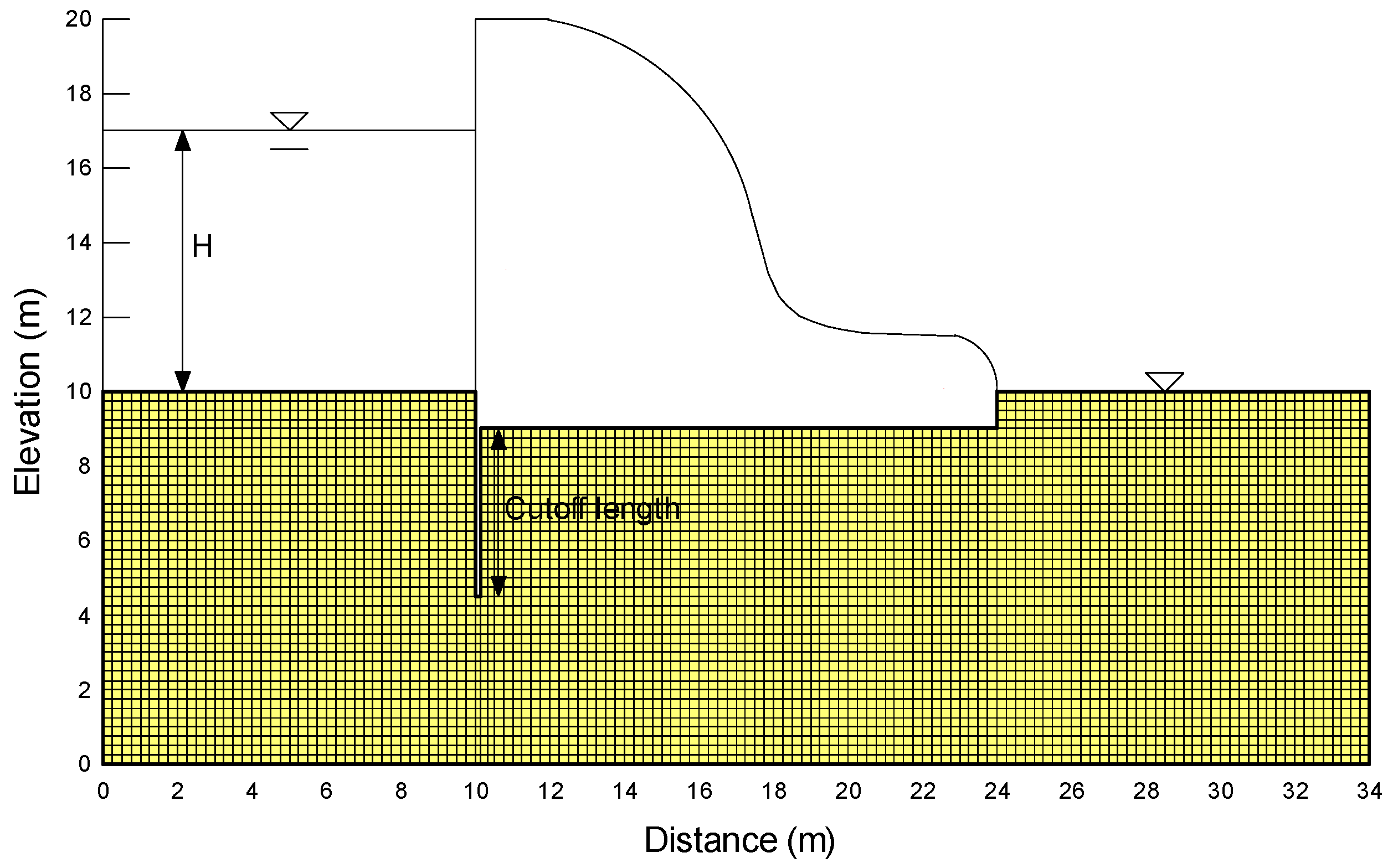
3.1. Soil Properties and Analysis Conditions

Many hydraulic infrastructures have been installed and operated in Korea for the purposes of water utilization and flood control. Notably, as a component of the 2008 Four Major Rivers Project, several barrages were established, which have subsequently faced safety issues such as water leakage, piping, and uplift pressure. Maintenance of these hydraulic structures requires evaluating their performance.

In order to consider the seepage behavior through the foundation soil of the water-retaining structure, an analysis model was constructed with a cutoff wall installed on the upstream side of the foundation, as shown in Figure 2. The water level $H$ of the upstream face can vary from 10 m to 20 m, i.e., the top elevation of the structure. The analysis model was constructed by referring to the case of an actual water-retaining structure located in Korea, which was dealt with by Jeon and Jung [37] and Bodda et al. [38].

Table 1. Statistical properties of soil parameters used for seepage analysis (lognormal distribution).

Parameter	${\mathit{\mu }}_{\mathit{k}}$(m/s)	${\mathit{C}\mathit{O}\mathit{V}}_{\mathit{k}}$	Autocorrelation Distance (m)
K	$1\times {10}^{-5}$	0.3, 0.5, 0.7, 1.0	$l_h=20$ $l_v=2$

summarizes the statistical properties of the soil parameters. The hydraulic conductivity $k$ was assumed to be characterized statistically by a lognormal distribution defined by a mean ${\mu }_k$ and a standard deviation ${\sigma }_k$ [39,40,41]. ${\mu }_k$ and ${\sigma }_k$ depend on the type of soil. Most of the riverbed materials in Korea are sandy soil (SP or SM in USCS). The selected ${\mu }_k$ (Table 1) is in the range of sandy soils. A generic range of the coefficient of variation (COV) for hydraulic conductivity, as suggested in the literature [42], is typically reported to be 68~90%, and this range was considered in this study. Since the directionality of the permeability characteristics is already considered by applying different autocorrelation distances in the vertical and horizontal directions, the hydraulic conductivity is assumed to be isotropic at any specific location. According to the results of a literature review by El-Ramly et al. [43], the autocorrelation distance is within a range of 10~40m in the horizontal direction, while in the vertical direction, it ranges from 1 to 3 m. As an illustration, an exponential autocorrelation structure with $l_h$ = 20 m and $l_v$ = 2 m was used.

3.2. Stochastic Simulations

The fragility curve can be developed by performing a series of Monte Carlo simulations while changing the water level at the upstream face of the water-retaining structure. A series of analyses were conducted using the generated random fields for each water level. Following the simulations, the mean and standard deviation of the output quantities were estimated. The main output quantities from each realization were the total seepage rate through the system $Q$, the exit hydraulic gradient $i_e$, and the uplift force $F$. The uplift force on the base of the water-retaining structure can be obtained by integrating the hydraulic pressure distribution along the base of the structure [27,31]. Accurate statistical responses were obtained from 10,000 sets of random fields that were generated for each case on the basis of the statistical information presented in Table 1.

In order to obtain the fragility curve directly from the MCS, seepage analysis must be performed based on 10,000 sets of random field realizations for each water level. Therefore, the computational workload increases proportionally to the number of water levels required to calculate the failure probability on the curve.

The case with ${COV}_k=0.5$, $l_h=20\mathrm{m}$, and $l_v=2\mathrm{m}$ for soil foundation was considered as a base set.

Figure 3 displays the histogram of MCS results for $Q$, $i_e$, and $F$ when $H$ is 17 m. In addition, the figure presents the results of fitting the MCS outcomes to a lognormal distribution, which includes the PDF and the CDF. The good match between the MCS results and the lognormal distribution is evident from these graphs. Previous research [23,24,34] has also shown that fitted lognormal distributions are well-suited to matching histograms of simulated seepage results. The adoption of a lognormal distribution for seepage results is based on the assumption that the hydraulic conductivity follows a lognormal probability distribution. The suggested fitting (Method B) employing a lognormal probability function may be affected by both the shape of the stochastic distribution of soil parameters and the stochastic distribution of outcomes. Of course, even if the seepage results do not follow a lognormal distribution, the method proposed in this study can still be applied as long as the seepage results can be represented by a probability distribution function.

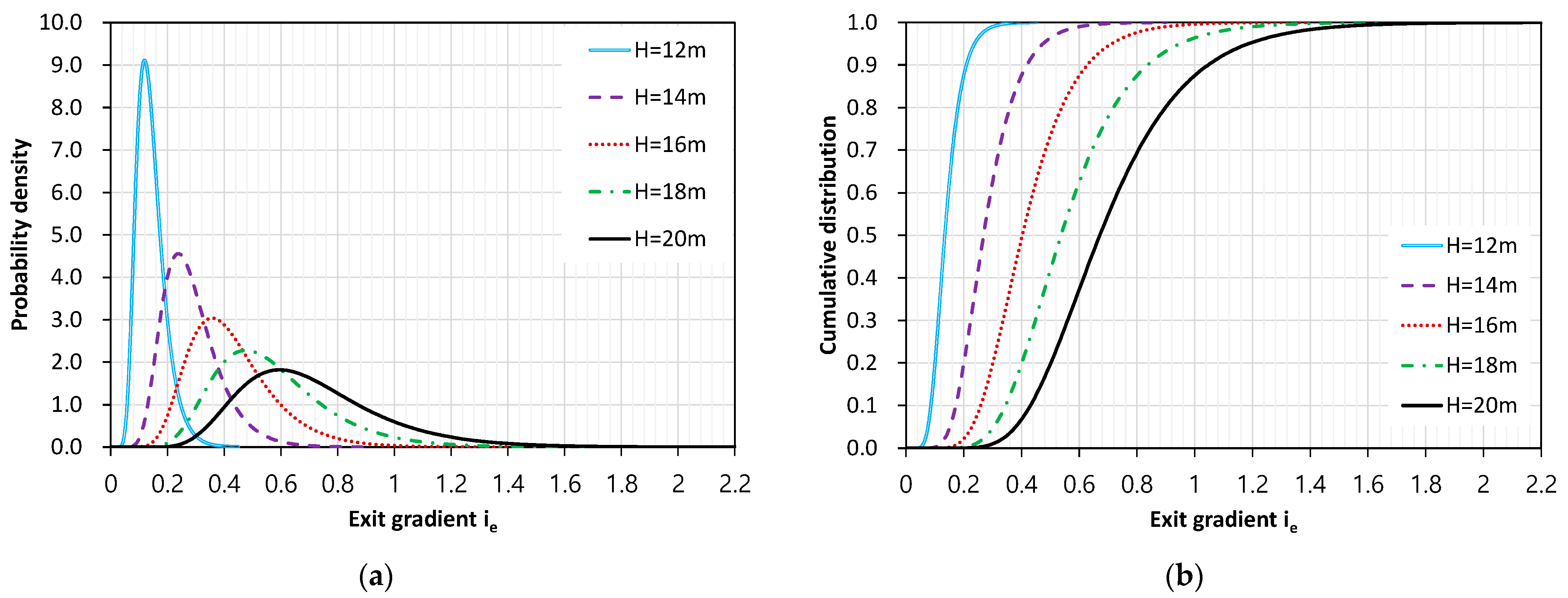
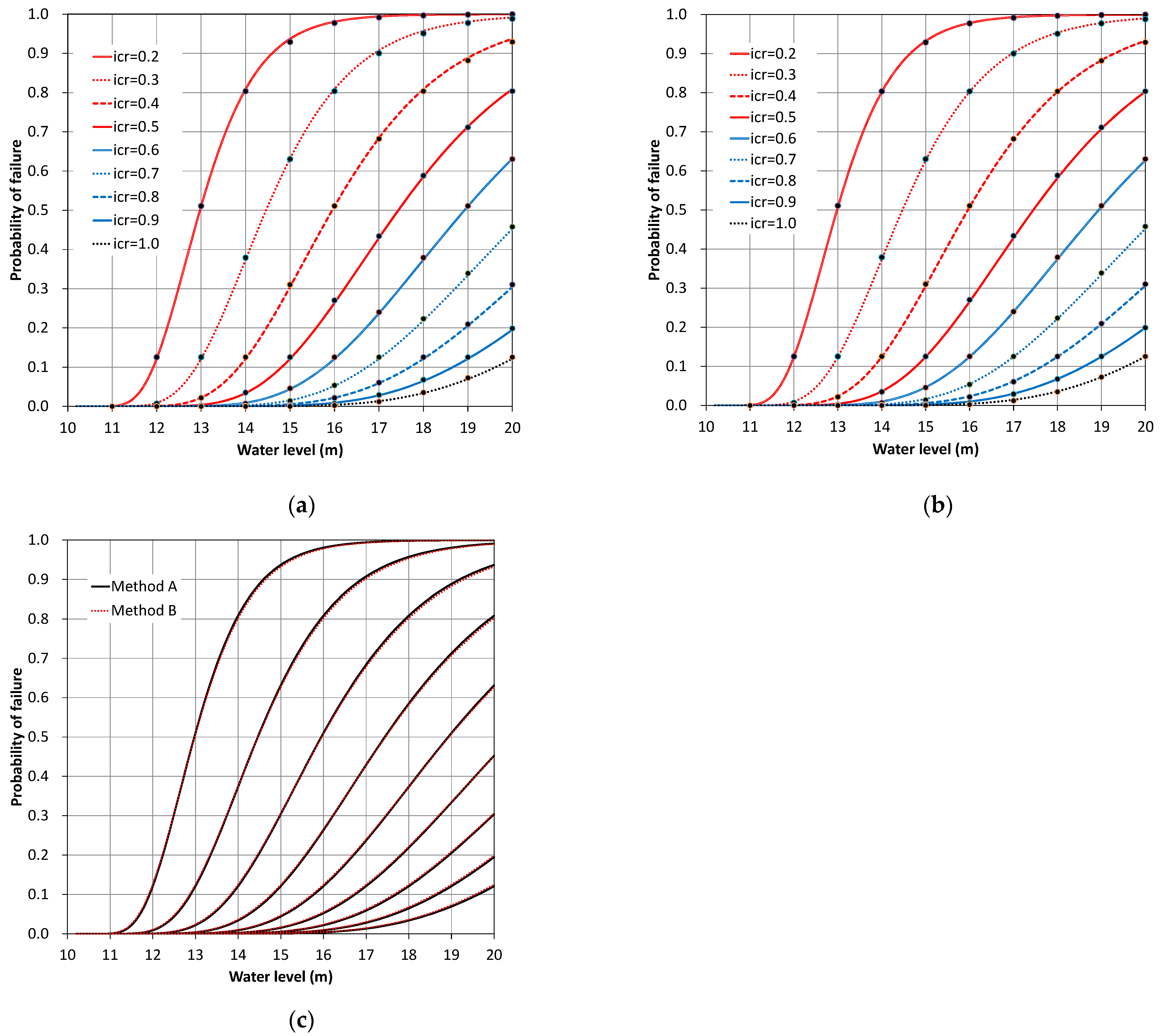
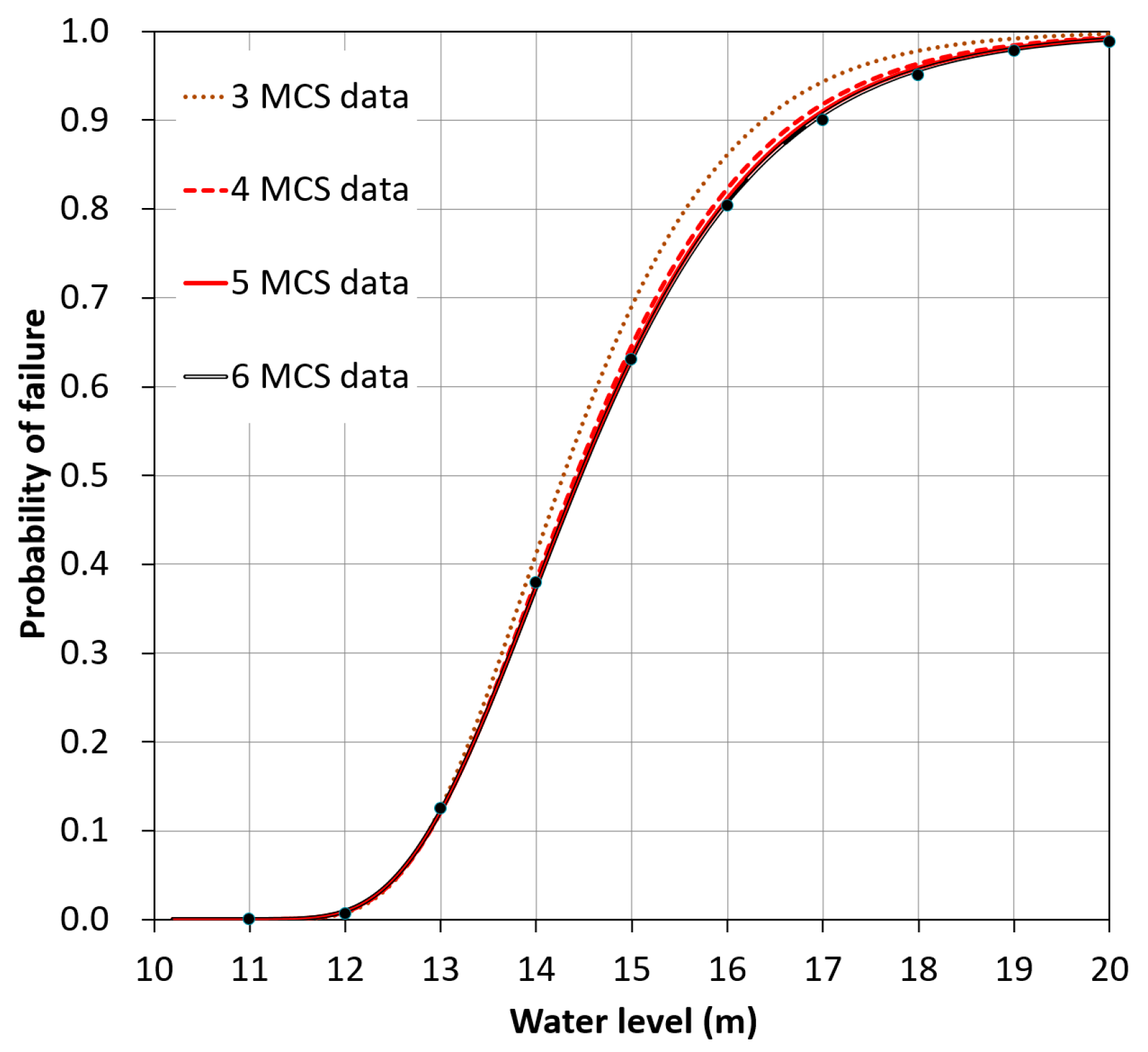
3.2.1. Fragility for Piping

Figure 4 displays the PDF and CDF of $i_e$. These were fitted from the MCS results for various water levels under the base set condition. As the water level increases, the $i_e$ also increases, causing the range of $i_e$ on the horizontal axis to shift to the right. In addition, the shape of the PDF becomes lower and wider as the water level increases. The PDF shows a lognormal distribution with a longer tail on the right side of its peak, indicating positive skewness.

Figure 5 illustrates the mean, standard deviation, and COV of $i_e$ estimated from both the MCS and fitted PDF with respect to the water level. As for the mean value, estimates obtained from the fitted lognormal distribution were consistent with those obtained from the MCS. There was a slight difference in the standard deviation as the water level increased, but the difference was not significant. As shown in Figure 5a,b, the estimated mean and standard deviation of $i_e$ increased proportionally with the water level. As the mean increased, the standard deviation also increased, resulting in a wider distribution that shifted to the right, as depicted in Figure 4a. To measure the dispersion of a probability distribution around the mean using the standard deviation, the effect of the mean must be removed. Therefore, the COV ($=\sigma /\mu$) was calculated from the mean and standard deviation, as shown in Figure 5c. The COV remained constant across all water levels, indicating that it was not influenced by the changing water levels. The COV obtained by the lognormal fit was only slightly higher than that obtained from the MCS. Root Mean Square Error (RMSE) was shown to indicate the quality of the lognormal fit to the MCS results.

The proposed methods were used to obtain the fragility curves for piping, as shown in Figure 6. These curves provide insights into the fragility of piping under different water levels. In Equation (7a), the limit state for piping is determined by the critical hydraulic gradient of soil. For most soils, the critical hydraulic gradient is around unity, and a high factor of safety against piping is usually advised for design purposes. Therefore, for illustrative purposes, a wide range of values for $i_{crit}$ was considered, as shown in Figure 6.

Figure 6a shows the fragility curve obtained using Method A, where the dots represent the failure probability calculated directly from the MCS. It is evident that the fragility curve obtained using Method A is in good agreement with that obtained from the MCS. However, calculating the failure probability directly from the MCS requires performing 10,000 seepage analyses for each water leve l, which can be time-consuming and requires significant computational resources. As a result, creating a smooth fragility curve with a small water level interval can be a time-intensive process that is proportional to the number of water levels.

On the other hand, since the value of $i_e$ is proportional to the head difference, the failure probability can be easily calculated from the ${\mu }_{i_e}\left(H\right)$ and ${\sigma }_{i_e}\left(H\right)$ corresponding to a specific water level $H$ by using Method A. In this study, the mean and standard deviation for $H=11\mathrm{m}$ and $H=20\mathrm{m}$ were estimated using the MCS. Then, ${\mu }_{i_e}\left(H\right)$ and ${\sigma }_{i_e}\left(H\right)$ for other water levels were linearly interpolated with a water level increment of $∆H=0.2\mathrm{m}$.

Figure 6b displays the fragility curves obtained through Method B. The dots in the figure represent the data obtained from MCS, which were used to fit the fragility function. The figure suggests that the lognormal CDF can effectively model the fragility of the water-retaining structure. Method B was used to calibrate Equation (20) from the MCS results for the piping failure mode, and the estimated $\theta$ and $\beta$ are summarized in

Table 2. Estimated $\theta$ and $\beta$ from the MCS results to calibrate Equation (20) for the piping failure mode of the water-retaining structure (Method B).

$i_{crit}$	0.2	0.3	0.4	0.5	0.6	0.7	0.8	0.9	1.0
$\theta$	2.981	4.470	5.960	7.450	8.940	10.427	11.913	13.392	14.862
$\beta$	0.346	0.346	0.346	0.346	0.346	0.346	0.346	0.345	0.345

.

Figure 6c illustrates a comparison between the fragility curves derived from Method A and Method B, indicating a strong agreement between the two results.

Method B is computationally efficient as it can estimate the fragility curve for the entire range of water levels based on a small dataset. Figure 7 illustrates the results of developing a fragility curve using 3, 4, 5, and 6 data points from the lowest water level among the 10 indicated by dots, considering the case of $i_{crit}=0.3$. From the figure, it is evident that even with a limited number of data points from only low water levels, the curve for the entire water level range is well-estimated.

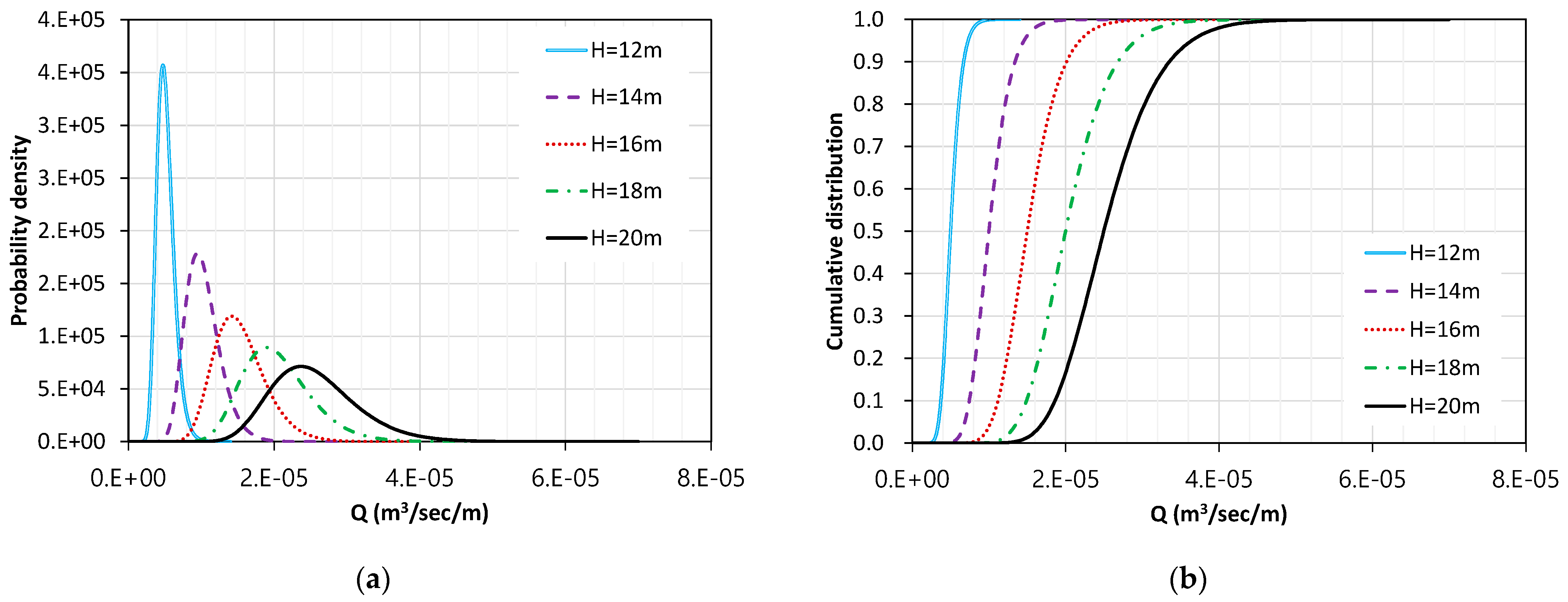
3.2.2. Fragility for Seepage Rate

Figure 8 illustrates the PDF and CDF of the lognormal distribution fitted to the seepage rate for different water levels. As the water level rises, the seepage rate also increases, which alters the distribution range on the horizontal axis. The PDF can be described as a lognormal distribution and has positive skewness. This is similar to the case of the exit hydraulic gradient. With the increase in the water level, the shape of the seepage rate PDF becomes flatter and wider.

Figure 9 displays the estimated mean, standard deviation, and COV values of the seepage rate with respect to the water level. The mean and standard deviation values estimated through the MCS were consistent with those obtained from the fitted lognormal distribution. As shown in Figure 9a,b, the mean and standard deviation of the seepage rate increased proportionally with the water level. The COV depicted in Figure 9c also remained constant, irrespective of the water level, but exhibited a smaller value compared to the COV of the exit hydraulic gradient. The allowable seepage rate is not clearly defined, as it depends on the purpose of water storage and the condition of the structure. However, failure may occur if the seepage rate exceeds a certain limit. An excessive seepage rate hinders the retention of available water, which reduces the benefits of constructing water-retaining structures. Therefore, the allowable seepage rate is prescribed and managed in terms of storage efficiency.

Figure 10 illustrates fragility curves based on different critical seepage rates. The dots on the graph represent failure probabilities calculated directly from MCS, indicating good agreement between the fragility curves generated by the proposed methods and the MCS results. When the critical seepage rate was 5 × 10⁻⁶ m³/s/m, the fragility curve had a steep slope, resulting in a significant increase in the probability of failure, even with a slight increase in water level (see Figure 10a,b). This suggests that the structure may experience reduced reliability, even with a small increase in the flood head. As the critical seepage rate increased, the fragility curve became less steep. For example, with a critical seepage rate of 2 × 10⁻⁵ m³/s/m, the probability of failure remained low, even when the water level reached 14 m. In addition, the degree of reduction in reliability due to the water level increase was small, even at higher water levels. Figure 10c compares the fragility curves obtained from Method A and Method B, showing that the two results are in good agreement.

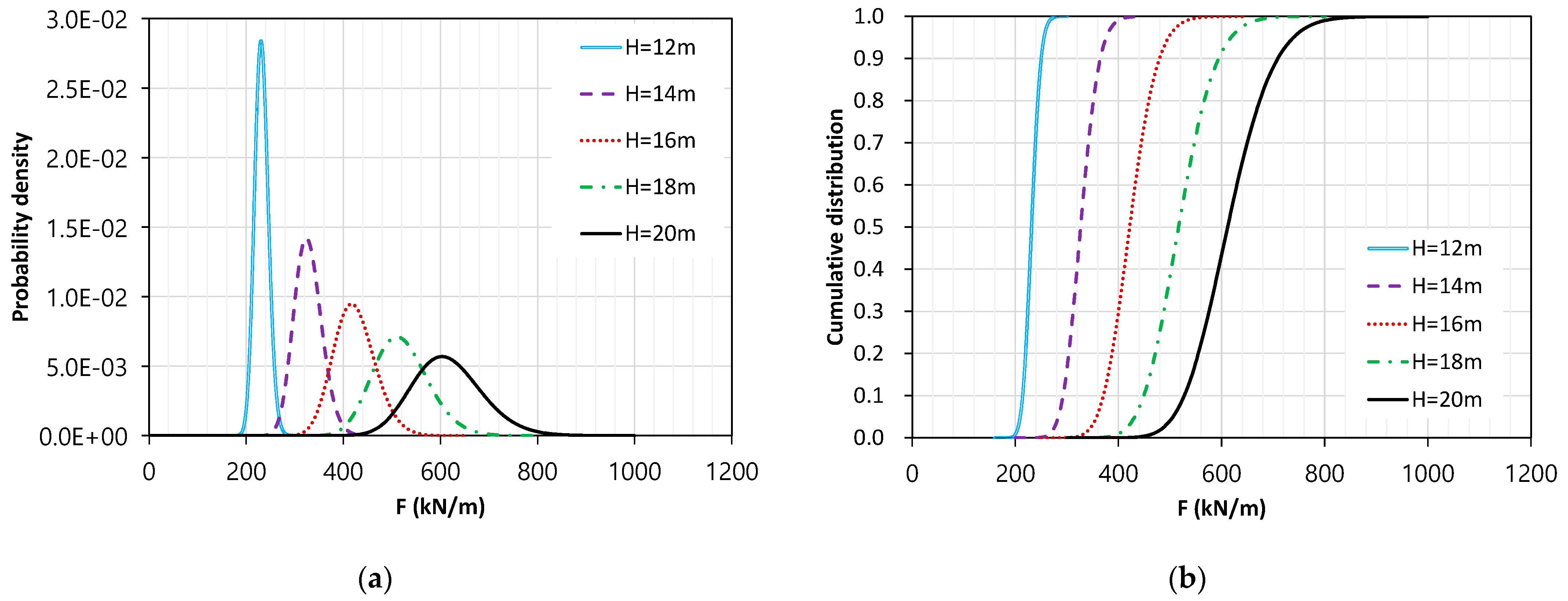
3.2.3. Fragility for Uplift Force

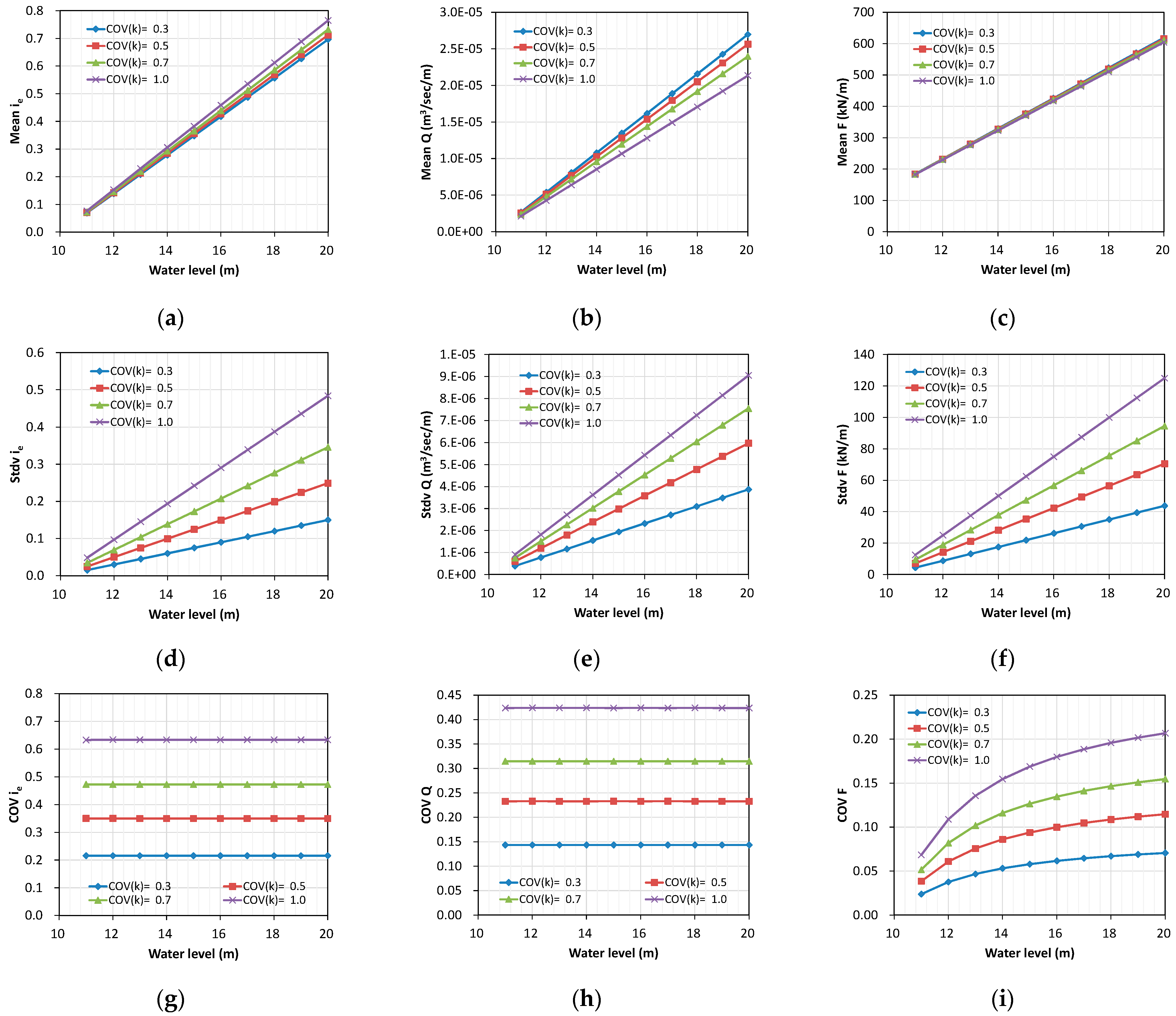
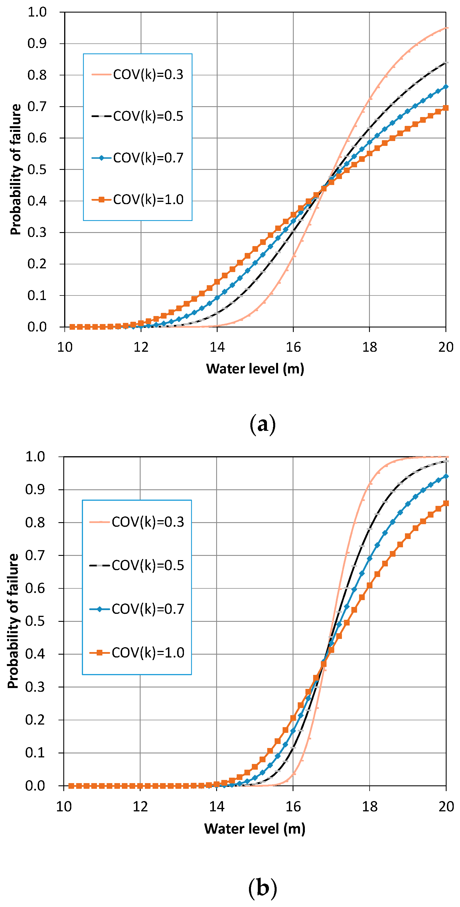
Figure 11 displays the fitted PDF and CDF of the uplift force acting on the structure’s base. As the water level rises, the uplift force also increases, resulting in a rightward shift of both the PDF and CDF on the horizontal axis. Although the probability distribution of the uplift force can be represented by a lognormal distribution, the PDF is relatively symmetrical, exhibiting a significantly smaller skewness coefficient compared to the cases of $i_e$ and $\mathrm{Q}$.

Figure 12a,b present the mean and standard deviation of the uplift force, respectively, with respect to the water level. These values can also be fitted with a straight line, making it easy to determine the mean and standard deviation for any other water level. While the COV of the uplift force is much lower than that of the exit hydraulic gradient and seepage rate (Figure 12c), it tends to increase as the water level rises. Unlike the exit hydraulic gradient and seepage rate, the COV of the uplift force did not change linearly with the water level. When the water level was at the bottom of the reservoir, where the head difference between the upstream and downstream faces was zero (i.e., $H=10\mathrm{m}$), the exit hydraulic gradient and seepage rate became zero. However, the uplift force acting on the structure’s base was not zero since the hydrostatic pressure persisted, even when $H=10\mathrm{m}$. In other words, the mean of the uplift force was not zero since the base of the structure was lower than the water level when $H=10\mathrm{m}$, resulting in the variation in COV ($=\sigma /\mu$) with the water level rising.

Figure 13 displays the fragility curve for the uplift force as the critical uplift force value is varied. Specifically, Figure 13a,b depict the fragility curves using Method A and Method B, respectively, demonstrating the effectiveness of both methods in developing the fragility curve for the uplift force. When the critical uplift force was small, the curve had a steep slope, indicating that a slight increase in water level could lead to a rapid rise in the failure probability. The failure probability eventually reached a value of 1.0 once the water level exceeded a certain threshold. Figure 13c compares the fragility curves obtained from Method A and Method B, showing that the two results match well.

3.3. Effect of ${COV}_k$ on the Fragility Curve

In this section, the effect of incorporating different values of ${COV}_k$ (i.e., the COV of hydraulic conductivity) was investigated, while the mean values of the hydraulic conductivity were fixed.

Figure 14 illustrates the results of estimating the mean and standard deviation of the seepage rate, exit hydraulic gradient, and uplift force by performing MCS while changing the ${COV}_k$. The figure shows that the ${COV}_k$ has a limited effect on the mean values, but the standard deviation is somewhat affected. Both the mean and standard deviation of the exit hydraulic gradient, seepage rate, and uplift force vary linearly with the water level.

Fragility curves can be developed for various potential damage states of a water-retaining structure not just for the structure’s failure state, by defining the undesirable limit state. For illustration purposes, the critical values used to define the limit state were selected as those the exit hydraulic gradient $i_{e\left(det\right)}$, uplift force $F_{\left(det\right)}$, and seepage rate $Q_{\left(det\right)}$ obtained from the deterministic analysis using the mean value of the hydraulic conductivity at $H=17\mathrm{m}$. This means that the prepared fragility curves represent the probability that the exit hydraulic gradient, uplift force, and seepage rate exceed the deterministic analysis values (when $H=17\mathrm{m}$) for each water level. Figure 15 shows the fragility curves for the piping, seepage rate, and uplift force developed using Method A. Figure 15 demonstrates that fragility curves can characterize the performance of structures that are challenging to predict intuitively because of the complexity of their behavior under various loading conditions.

The fluctuation range of soil variation also has a great influence on the fragility curve. Since there are various factors that affect the fragility curve, additional research is needed.

3.4. Effect of Variation in the Cutoff Length

In this section, the effect of variation in cutoff length on the fragility curve was examined for the basic condition while other conditions were fixed. The proposed Method A was applied to efficiently build fragility curves with minimal computation. Monte Carlo simulations were conducted for different cutoff lengths, considering two water levels: $H=11\mathrm{m}$ and $20\mathrm{m}$. Subsequently, the mean and standard deviation of the exit gradient, uplift force, and seepage rate were estimated. As anticipated, increasing the length of the cutoff resulted in a significant reduction in the mean values of the exit gradient, uplift force, and seepage rate. However, no significant variations were observed in the standard deviation of the exit gradient, uplift force, and seepage rate.

Figure 16 presents typical realizations of the hydraulic conductivity fields and their corresponding results from the seepage analysis when $H$ is 20 m. In the figures, lighter regions represent lower hydraulic conductivity values, while darker regions indicate higher hydraulic conductivity values.

The fragility curves presented in Figure 17 depict the impact of adjusting the cutoff length on piping, seepage rate, and uplift force. To maintain simplicity, the critical values used to define the limit state remain consistent with those employed in Section 3.3. The findings from Figure 17 demonstrate that adjusting the cutoff length can effectively enhance the water-retaining structure’s resistance against seepage, improving its overall performance.

4. Discussion

Fragility curves and fragility functions are both utilized in risk analysis to depict the relationship between a specific intensity measure and the possibility of a certain level of damage or failure for a structure. The term ‘fragility curve’ is often used interchangeably with ‘fragility function’, but they differ in mathematical form [6]. A fragility curve is a graphical representation of the relationship between a measure of intensity and the probability of exceeding a certain level of damage or failure. On the other hand, a fragility function is a mathematical equation that describes the probability of exceeding a certain level of damage or failure as a function of an intensity measure.

Both methods used in this study show the relationship between the water level and the failure probability of a water-retaining structure. However, Method A can be called a fragility curve because it is a graphical representation based on a set of discrete points. On the other hand, Method B can be called a fragility function because it is expressed in the form of an equation. From the perspective of computation only, Method A can be considered more efficient than Method B, as it only needs to perform the MCS for two water levels. On the other hand, Method B has the advantage of being expressed in the form of a function.

By utilizing the suggested methods, it becomes convenient to generate fragility curves for water-retaining structures, taking into account the length and placement of the cutoff wall. These prepared fragility curves are valuable for risk assessment, design, and decision-making purposes, as they offer information to evaluate the performance of the water-retaining structure under various water level conditions. Through the analysis of fragility curves, we can gain a deeper understanding of the potential consequences stemming from extreme flood scenarios and make well-informed decisions regarding measures for mitigation and emergency planning. Although this study is currently limited to research on seepage through soil beneath water-retaining structures, it will provide valuable insights to engineers interested in developing fragility curves through numerical analysis.

The 2D model used in this study implies that the out-of-plane spatial autocorrelation distance is infinite; thus, soil properties are constant in this direction. Compared with 2D analysis, 3D allows the flow greater freedom to avoid the low permeability zones. The influence of 3D is, therefore, to reduce the overall randomness of the results observed from one realization to the next. This was manifested in a reduced mean and standard deviation of the seepage results as compared with 2D. However, according to previous studies by Griffiths and Fenton [17,28] involving seepage through 2D and 3D random fields, the differences were not great and indicated that 2D studies in random soils will lead to conservative results while giving sufficient accuracy [17]. The 3D studies are considerably more intensive computationally than their 2D counterparts but had the modeling advantage of removing the requirement of planar flow. In addition, Griffiths and Fenton [17,28] showed that 3D seepage results can also be well represented by a lognormal distribution, so the method proposed in this study can be efficiently applied to 3D seepage models.

5. Summary and Conclusions

Extensive research has been conducted to accurately analyze probabilistic seepage underneath water-retaining structures, and highly advanced analysis models that consider the effect of stochastic soil permeability have been developed. However, systematic studies on the development of fragility curves using these analysis models are exceedingly rare. This study introduced two efficient methods to develop fragility curves of water-retaining structures, allowing for the assessment of failure probabilities related to important quantities such as steady-state seepage rates, exit gradients, and uplift forces. The following conclusions were drawn from the analyses:

1. The appropriate probability distribution function of the exit hydraulic gradient, uplift force, and seepage rate obtained from the MCS results for seepage through the soil beneath a water-retaining structure can be selected from probability distribution fitting. Once the mean and standard deviation of seepage output, the parameters of the PDF, are evaluated for one or two water levels from the MCS, the probability distribution is specified. Then, the mean and standard deviation can be evaluated for other water levels from the simple linear influence of the water head difference between the upstream and downstream faces on equations;

2. The fragility curves obtained using the proposed methods agreed well with the results from the MCS, demonstrating the effectiveness of these methods in predicting the performance of water-retaining structures. By utilizing these methods, it is possible to develop fragility curves with less computational effort by reducing the number of time-consuming and computationally intensive MCS operations. More importantly in terms of efficiency, these methods can provide continuous fragility information based on water levels with minimal effort;

3. Fragility curves can be developed for various potential damage states of a water-retaining structure, not just for the structure’s failure state, by defining an undesirable limit state as illustrated in this study. Therefore, fragility curves can serve as decision-making tools during disasters, which are essential for emergency preparedness for disaster reduction.

References

1. USACE. Risk-Based Analysis for Flood Damage Reduction Studies; Engineer Manual 1110-2-1619; US Army Corps of Engineers: Washington, DC, USA, 1996; Available online: https://apps.dtic.mil/sti/pdfs/ADA401763.pdf (accessed on 27 November 2023).
2. Simm, J.; Tarrant, O. Development of fragility curves to describe the performance of UK levee systems. In Proceedings of the Twenty-Sixth International Congress on Large Dams, Vienna, Austria, 1–7 July 2018. [Google Scholar]
3. Rossi, N.; Bačić, M.; Kovačević, M.S.; Librić, L. Development of fragility curves for piping and slope stability of river levees. Water 2021, 13, 738. [Google Scholar] [CrossRef]
4. Kennedy, R.P.; Cornell, C.A.; Campbell, R.D.; Kaplan, S.; Perla, H.F. Probabilistic seismic safety study of an existing nuclear power plant. Nucl. Eng. Des. 1980, 59, 315–338. [Google Scholar] [CrossRef]
5. Tsompanakis, Y.; Lagaros, N.D.; Psarropoulos, P.N.; Georgopoulos, E.C. Probabilistic seismic slope stability assessment of geostructures. Struct. Infrastruct. Eng. 2010, 6, 179–191. [Google Scholar] [CrossRef]
6. Porter, K. A Beginner’s Guide to Fragility, Vulnerability, and Risk; University of Colorado Boulder: Boulder, CO, USA, 2018; Available online: https://www.sparisk.com/pubs/Porter-beginners-guide.pdf (accessed on 27 November 2023).
7. Cho, S.E. Failure distribution analysis of shallow landslides under rainfall infiltration based on fragility curves. Landslides 2020, 17, 79–91. [Google Scholar] [CrossRef]
8. Vorogushyn, S.; Merz, B.; Apel, H. Development of dike fragility curves for piping and micro-instability breach mechanisms. Nat. Hazards Earth Syst. Sci. 2009, 19, 1383–1401. [Google Scholar] [CrossRef]
9. Wu, X.Z. Development of fragility functions for slope instability analysis. Landslides 2015, 12, 165–175. [Google Scholar] [CrossRef]
10. Martinović, K.; Reale, C.; Gavin, K. Fragility curves for rainfall-induced shallow landslides on transport networks. Can. Geotech. J. 2018, 55, 852–861. [Google Scholar] [CrossRef]
11. McKenna, G.; Argyroudis, S.A.; Winter, M.G.; Mitoulis, S.A. Multiple hazard fragility analysis for granular highway embankments: Moisture ingress and scour. Transp. Geotech. 2021, 26, 100431. [Google Scholar] [CrossRef]
12. Hall, J.W.; Dawson, R.J.; Sayers, P.B.; Rosu, C.; Chatterton, J.B.; Deakin, R. A methodology for national-scale flood risk assessment. Proc. Inst. Civ. Eng.-Water Marit. Eng. 2003, 156, 235–247. [Google Scholar] [CrossRef]
13. Dawson, R.J.; Hall, J.; Sayers, P.; Bates, P.; Rosu, C. Sampling-based flood risk analysis for fluvial dike systems. Stoch. Environ. Res. Risk Assess. 2005, 19, 388–402. [Google Scholar] [CrossRef]
14. Wojciechowska, K.; Pleijter, G.; Zethof, M.; Havinga, F.; Haaren, D.V.; Ter Horst, W. Application of fragility curves in operational flood risk assessment. In Proceedings of the 5th International Symposium on Geotechnical Safety and Risk, Rotterdam, The Netherlands, 13–16 October 2015; IOS Press: Amsterdam, The Netherlands, 2015; pp. 528–534. [Google Scholar] [CrossRef]
15. Mainguenaud, F.; Peyras, L.; Khan, U.T.; Carvajal, C.; Sharma, J.; Beullac, B. A probabilistic approach to levee reliability based on sliding, backward erosion and overflowing mechanisms: Application to an inspired Canadian case study. J. Flood Risk Manag. 2023, 16, e12921. [Google Scholar] [CrossRef]
16. Fenton, G.A.; Griffiths, D.V. Extreme hydraulic gradient statistics in stochastic earth dam. J. Geotech. Geoenviron. Eng. 1997, 123, 995–1000. [Google Scholar] [CrossRef]
17. Griffiths, D.V.; Fenton, G.A. Probabilistic analysis of exit gradients due to steady seepage. J. Geotech. Geoenviron. Eng. 1998, 124, 789–797. [Google Scholar] [CrossRef]
18. Srivastava, A.; Sivakumar Babu, G.L.; Haldar, S. Influence of spatial variability of permeability property on steady state seepage flow and slope stability analysis. Eng. Geol. 2010, 110, 93–101. [Google Scholar] [CrossRef]
19. Ahmed, A.A. Stochastic analysis of seepage under hydraulic structures resting on anisotropic heterogeneous soils. J. Geotech. Geoenviron. Eng. 2012, 139, 1001–1004. [Google Scholar] [CrossRef]
20. Cho, S.E. Probabilistic analysis of seepage that considers the spatial variability of permeability for an embankment on soil foundation. Eng. Geol. 2012, 133–134, 30–39. [Google Scholar] [CrossRef]
21. Liu, L.L.; Cheng, Y.M.; Jiang, S.H.; Zhang, S.H.; Wang, X.M.; Wu, Z.H. Effects of spatial autocorrelation structure of permeability on seepage through an embankment on a soil foundation. Comput. Geotech. 2017, 87, 62–75. [Google Scholar] [CrossRef]
22. Tan, X.; Wang, X.; Khoshnevisan, S.; Hou, X.; Zha, F. Seepage analysis of earth dams considering spatial variability of hydraulic parameters. Eng. Geol. 2017, 228, 260–269. [Google Scholar] [CrossRef]
23. Hekmatzadeh, A.A.; Zarei, F.; Johari, A.; Haghighi, A.T. Reliability analysis of stability against piping and sliding in diversion dams, considering four cutoff wall configurations. Comput. Geotech. 2018, 98, 217–231. [Google Scholar] [CrossRef]
24. Johari, A.; Heydari, A. Reliability analysis of seepage using an applicable procedure based on stochastic scaled boundary finite element method. Eng. Anal. Bound. Elem. 2018, 94, 44–59. [Google Scholar] [CrossRef]
25. Liu, K.; Vardon, P.J.; Hicks, M.A. Probabilistic analysis of seepage for internal stability of earth embankments. Environ. Geotech. 2019, 6, 294–306. [Google Scholar] [CrossRef]
26. Chi, F.; Breul, P.; Carvajal, C.; Peyras, L. Stochastic seepage analysis in embankment dams using different types of random fields. Comput. Geotech. 2023, 162, 105689. [Google Scholar] [CrossRef]
27. Griffiths, D.V.; Fenton, G.A. Seepage beneath water retaining structures founded on spatially random soil. Géotechnique 1993, 43, 577–587. [Google Scholar] [CrossRef]
28. Griffiths, D.V.; Fenton, G.A. Three-dimensional seepage through spatially random soil. J. Geotech. Geoenviron. Eng. 1997, 123, 153–160. [Google Scholar] [CrossRef]
29. Robbins, B.A.; Griffiths, D.V.; Fenton, G.A. Random finite element analysis of backward erosion piping. Comput. Geotech. 2021, 138, 104322. [Google Scholar] [CrossRef]
30. Cho, S.E. Probabilistic assessment of seepage stability of soil foundation under water retaining structures by fragility curves. J. Korean Geotech. Soc. 2021, 37, 41–54. [Google Scholar] [CrossRef]
31. Cho, S.E. Probabilistic seepage analysis by the finite element method considering spatial variability of soil permeability. J. Korean Geotech. Soc. 2011, 27, 93–104. [Google Scholar] [CrossRef]
32. Lacasse, S.; Nadim, F. Uncertainties in characterizing soil properties. In Proceedings of the Uncertainty 96, Madison, WI, USA, 31 July–3 August 1996; ASCE: Reston, VA, USA, 1996; pp. 49–75. [Google Scholar]
33. Vanmarcke, E.H. Random Fields: Analysis and Synthesis; World Scientific: Singapore, 1983. [Google Scholar]
34. Fenton, G.A.; Griffiths, D.V. Risk Assessment in Geotechnical Engineering; John Wiley & Sons: Hoboken, NJ, USA, 2008. [Google Scholar]
35. Kennedy, R.P.; Ravindra, M.K. Seismic fragilities for nuclear power plant risk studies. Nucl. Eng. Des. 1980, 79, 47–68. [Google Scholar] [CrossRef]
36. Baker, J.W. Efficient analytical fragility function fitting using dynamic structural analysis. Earthq. Spectra 2015, 31, 579–599. [Google Scholar] [CrossRef]
37. Jeon, O.H.; Jung, W.Y. Fragility analysis of weir structure subjected to flooding water damage. Int. J. Civ. Environ. Eng. 2018, 12, 75–80. Available online: https://publications.waset.org/10008936/pdf (accessed on 27 November 2023).
38. Bodda, S.S.; Gupta, A.; Ju, B.S.; Jung, W.Y. Fragility of a weir structure due to scouring. Comput. Eng. Phys. Model. 2020, 3, 1–15. [Google Scholar] [CrossRef]
39. Freeze, R.A. A stochastic-conceptual analysis of one-dimensional groundwater flow in nonuniform homogeneous media. Water Resour. Res. 1975, 11, 725–741. [Google Scholar] [CrossRef]
40. Hoeksema, R.J.; Kitanidis, P.K. Analysis of the spatial structure of properties of selected aquifers. Water Resour. Res. 1985, 21, 563–572. [Google Scholar] [CrossRef]
41. Sudicky, E.A. A natural gradient experiment on solute transport in a sand aquifer: Spatial variability of hydraulic conductivity and its role in the dispersion process. Water Resour. Res. 1986, 22, 2069–2083. [Google Scholar] [CrossRef]
42. Duncan, J.M. Factors of safety and reliability in geotechnical engineering. J. Geotech. Geoenviron. Eng. 2000, 126, 307–316. [Google Scholar] [CrossRef]
43. El-Ramly, H.; Morgenstern, N.R.; Cruden, D.M. Probabilistic stability analysis of a tailings dyke on presheared clay-shale. Can. Geotech. J. 2003, 40, 192–208. [Google Scholar] [CrossRef]
Figure 1. Procedures for fragility curve development by Method A.
Water 15 04165 g001
Figure 2. Finite element discretization of the soil beneath the water-retaining structure (modified from [31]).
Water 15 04165 g002
Figure 3. Results of the MCS ( C O V k = 0.5 , l h = 20   m , l v = 2   m , H = 17   m ), PDF, and CDF: (a) exit gradient; (b) seepage rate; (c) uplift force.
Water 15 04165 g003
Figure 4. Results of the MCS ( C O V k = 0.5 , l h = 20   m , l v = 2   m ): PDF and CDF of the exit gradient at different water levels: (a) PDF; (b) CDF.
Water 15 04165 g004
Figure 5. Variation in the estimated mean, standard deviation, and COV of the exit gradient with the water level ( C O V k = 0.5 , l h = 20   m , l v = 2   m ): (a) Variation in the mean of the exit gradient (RMSE = 3.0496 × 10⁻⁴); (b) Variation in the standard deviation of the exit gradient (RMSE = 3.354 × 10⁻³); (c) Variation in the COV of the exit gradient (RMSE = 7.2841 × 10⁻³).
Water 15 04165 g005
Figure 6. Fragility curves for piping with respect to varying critical hydraulic gradients ( C O V k = 0.5 , l h = 20   m , l v = 2   m ; dots are the MCS results): (a) Method A; (b) Method B; (c) Comparison of fragility curves obtained from Method A and Method B.
Water 15 04165 g006
Figure 7. Function fitting results by Method B according to the number of data ( i c r i t = 0.3).
Water 15 04165 g007
Figure 8. Results of the MCS ( C O V k = 0.5 , l h = 20   m , l v = 2   m ): the PDF and CDF of the seepage rate at different water levels: (a) PDF; (b) CDF.
Water 15 04165 g008
Figure 9. Variation in the estimated mean, standard deviation, and COV of the seepage rate with the water level ( C O V k = 0.5 , l h = 20   m , l v = 2   m ): (a) variation in the mean of the seepage rate (RMSE = 0.0); (b) variation in the standard deviation of the seepage rate (RMSE = 1.1836 × 10⁻⁹); (c) variation in the COV of the seepage rate (RMSE = 7.9706 × 10⁻⁵).
Water 15 04165 g009
Figure 10. Fragility curves for the seepage rate with respect to varying critical seepage rates ( C O V k = 0.5 , l h = 20   m , l v = 2   m ; dots are the MCS results): (a) Method A; (b) Method B; (c) Comparison of fragility curves obtained from Method A and Method B.
Water 15 04165 g010
Figure 11. Results of the MCS ( C O V k = 0.5 , l h = 20   m , l v = 2   m ): the PDF and CDF of the uplift force at different water levels: (a) PDF; (b) CDF.
Water 15 04165 g011
Figure 12. Variation in the estimated mean, standard deviation, and COV of the uplift force with the water level ( C O V k = 0.5 , l h = 20   m , l v = 2   m ): (a) Variation in the mean of uplift force (RMSE = 1.4511 × 10⁻²); (b) Variation in the standard deviation of uplift force (RMSE = 3.9815 × 10⁻¹); (c) Variation in the COV of uplift force (RMSE = 7.4303 × 10⁻⁴).
Water 15 04165 g012
Figure 13. Fragility curves for uplift with respect to varying critical uplift forces ( C O V k = 0.5 , l h = 20   m , l v = 2   m ; dots are the MCS results): (a) Method A; (b) Method B; (c) Comparison of fragility curves obtained from Method A and Method B.
Water 15 04165 g013
Figure 14. Influence of the C O V k on the estimated mean, standard deviation, and COV of exit gradient, seepage rate, and uplift force obtained from simulations (fixed l h = 20   m and l v = 2   m ); (a) mean of exit gradient; (b) mean of seepage rate; (c) mean of uplift force; (d) standard deviation of exit gradient; (e) standard deviation of seepage rate; (f) standard deviation of uplift force; (g) COV of exit gradient; (h) COV of seepage rate; (i) COV of uplift force.
Water 15 04165 g014
Figure 15. Fragility curves for the seepage with respect to varying C O V k (fixed l h = 20   m and l v = 2   m ): (a) fragility curves for the piping ( s c r i t = i e ( d e t ) = 0.48 ); (b) fragility curves for the uplift ( s c r i t = F ( d e t ) = 475   k N / m ); (c) fragility curves for the seepage rate ( s c r i t = Q ( d e t ) = 1.949 × 10 5   m 3 / s / m ).
Water 15 04165 g015aWater 15 04165 g015b
Figure 16. Typical realizations of the random field and the corresponding analysis results when H is 20 m (fixed C O V k = 0.5 , l h = 20   m and l v = 2   m ): (a) cutoff length = 0 m; (b) cutoff length = 1.5 m; (c) cutoff length = 3.0 m; (d) cutoff length = 4.5 m.
Water 15 04165 g016aWater 15 04165 g016b
Figure 17. Fragility curves for the seepage with respect to varying cutoff length (fixed C O V k = 0.5 , l h = 20   m and l v = 2   m ): (a) fragility curves for the piping ( i c r = 0.48 ); (b) fragility curves for the uplift ( F c r = 475   k N / m ); (c) fragility curves for the seepage rate ( Q c r = 1.949 × 10 5   m 3 / s / m ).
Water 15 04165 g017aWater 15 04165 g017b