1. Introduction
The increasing threat of drought resulting from climate change and abnormal weather has led to growing expectations for measures such as irrigation, embankment of intake stations, multipurpose dams, and water supply dams [
1,
2,
3] to ensure stable water supply in the Yeongsan and Seomjin river basins. To address long-term water shortages at the national level, the Ministry of Land, Transport, and Maritime Affairs (MLTM) has been established, which predicts demand and supply for all basins nationwide. However, the focus is mainly on national rivers and multipurpose dams, while local and small rivers are relatively underdeveloped [
4,
5,
6,
7].
Water demand forecasting plays a critical role in determining the production plan for clean water at water treatment plants, the operation plan for water pumps, and the operation plan for reservoirs. Proper utilization of the predicted water demand value can lead to cost reductions in operation, production, and transportation. On the other hand, if high-accuracy water demand prediction is not achieved, excessive water may be transferred from the water treatment plant to the reservoir, leading to inefficient pump operation and excessive power consumption. Furthermore, the water level in the reservoir may not be properly adjusted due to the excessive water supply, which can result in various problems [
6,
8,
9,
10,
11].
In the context of large-scale water supply management, it is important to have accurate water demand forecasts to plan pumping operations and optimize costs. Previous studies have compared the performance of the adaptive neuro-fuzzy inference system (ANFIS) and the auto-regressive (AR) model for water demand prediction, and found that the AR model provides better prediction results. Typically, AR models are used for short-term forecasting, where general trends and periodic patterns on an annual, weekly, and daily basis can be identified. However, the AR model is not suitable for predicting water demand with complex cycle components that are combined in various patterns. This has been highlighted in previous studies [
6,
12,
13,
14,
15].
To address these issues, Tabesh and Dini (2009) [
16] proposed a water demand prediction model that considers the influence of external factors such as weather and water level data. They applied an artificial neural network (ANN) model, which is a nonlinear model. Choi et al. (2009) [
17] suggested that an AI-based model, specifically a multi-layer perceptron, would be appropriate. Firat et al. (2010) [
18] applied generalized regression neural network (GRNN) and cascade correlation neural network (CCNN) isometric neural network models to predict water demand. More improved prediction results have been confirmed by comparing machine learning- and deep learning-based prediction models with AR models [
10,
19,
20,
21].
Since water demand forecasting is essential for optimal water resource management, many studies have applied and developed various methods for accurate forecasting. It is also necessary to study whether decision makers should quantitatively supply water demand. There is a need for research to support decision makers in determining how much water demand will be sufficient or insufficient and how much supply there will be in the future.
The current state of drought situation management in Korea can be grasped based on the standard manual for crisis management, ⌈Drought disaster⌋. And to detect signs related to a drought crisis or to assess the level of risk when a crisis is expected to occur, a crisis alert is issued. The four stages of crisis management are attention (blue) → caution (yellow) → alert (orange) → severe (red). In the case of a drought disaster, there are criteria for each level of crisis alert, and situation management takes this into consideration [
3,
10,
22]. However, the current quantitative standards for drought management are ambiguous, making it difficult for decision makers to make judgments.
The purpose of this study is to minimize drought damage through prompt and efficient response, in line with the goals of the Drought Disaster Crisis Management Basic Direction [
3,
4,
5,
6,
7,
10,
22]. A prediction model was developed using long short-term memory (LSTM) and deep neural network (DNN) models to enable decision makers to quantitatively supply water demand. To establish a quantitative standard, the probability density function (PDF) for the water demand data was calculated, along with the probability of including the random variable for the interval. Based on this, the cumulative distribution function (CDF) was used to calculate the probability that a given random variable is less than or equal to a specific value, and standards were established according to the drought crisis warning stage. Decision tree (DT) and random forest (RF) models were used to roughly estimate the supply scale of water demand in the near future based on the established criteria. In this way, water demand prediction is essential in terms of optimal water resource management and energy savings. Therefore, we attempted to apply machine learning and deep learning to accurately predict water damage. The model proposed in this study can be used to determine the amount of supply by predicting consumers’ water demand and to establish optimal operation plans. It can also significantly contribute to reducing power consumption and energy at the national level.
2. Methods and Materials
2.1. Study Area
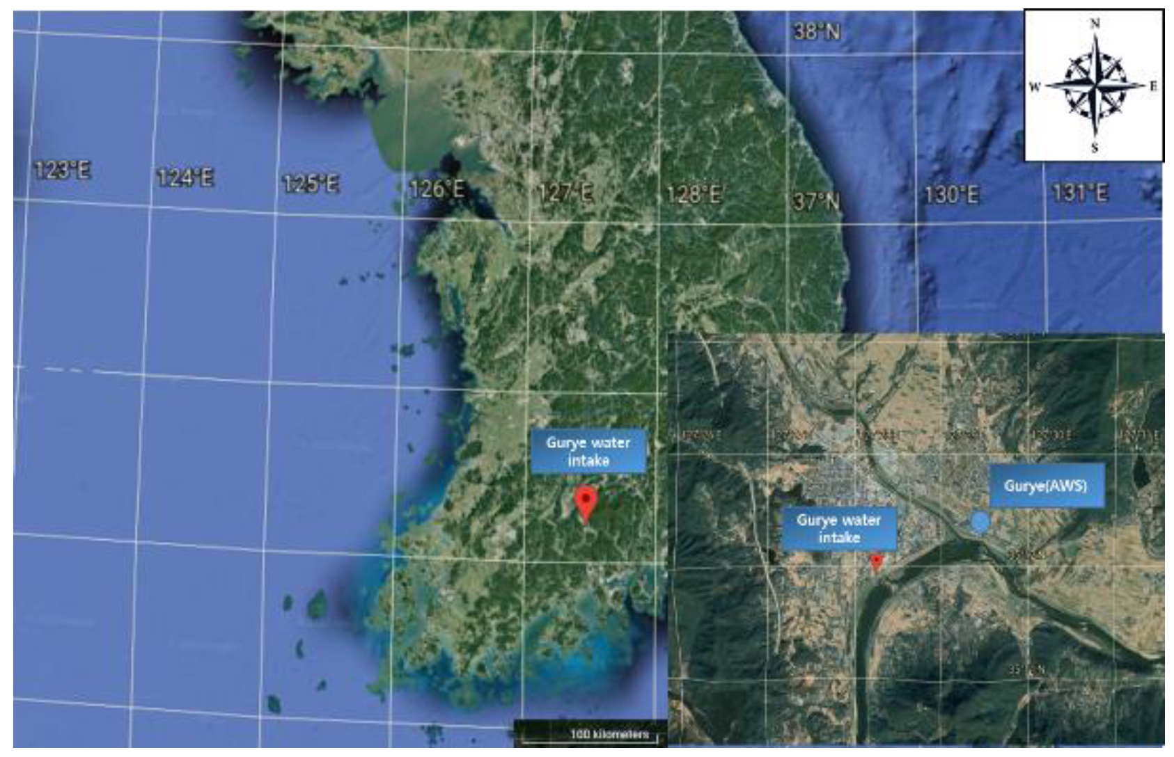
In the Seomjin river basin, Gokseong, Gurye, and Gwangyang occupy most of the area, and Suncheon, Hwasun, and Boseong make up some of it. The water quality of the Seomjin river is close to the first-class level at all points including Gurye, the representative point, and Namwon and Hadong. In addition, since water for agricultural use is supplied using a water conveyance tunnel, continuous monitoring of drought and water quality is an essential point. Gurye intake station has the distinction of being an intermediate point from the Seomjin river dam to the Seomjin river estuary and forms abundant flow as a confluence point of nearby small rivers. It is also an important facility that can respond to drought and water quality changes and stably supply high-quality water demand. The intake ability of Gurye intake station is 11,000 (m
3/day), the intake volume is 9098 (m
3/day), the water supply area is Gurye, and the population supply is 9881 people (
Figure 1).
Data from 1 January 2004 to 31 December 2021on independent variables such as water demand, average temperature, and minimum temperature were used.
Table 1 shows the basic statistics of dependent and independent variable data. Meteorological data and water demand data can be downloaded from the Meteorological Data Open Portal operated by the Korea Meteorological Administration (
https://data.kma.go.kr/cmmn/main.do, accessed on 31 December 2021).
2.2. Flow Chart of the Present Study’s Procedure
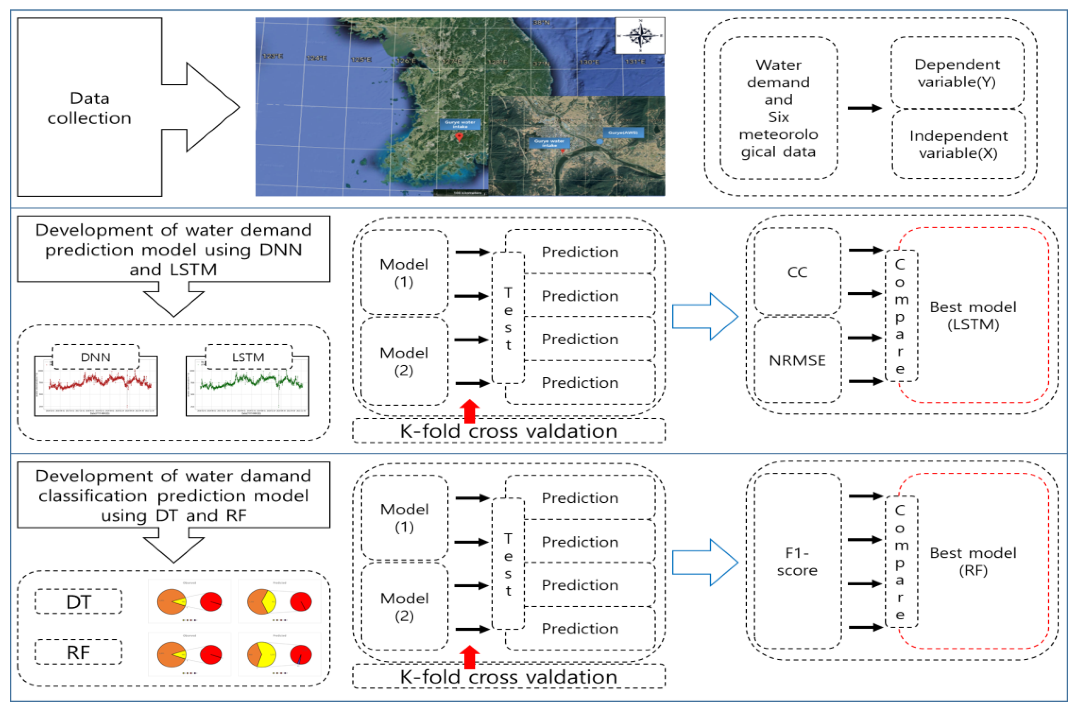
In this study, an AI-based water demand forecasting model was developed to quantitatively predict the water demand of Gurye intake station. Crisis Alert Levels (scale) were set using PDF and CDF, and an AI-based classification model was applied based on the set criteria. The flow of this study is explained in detail as follows (
Figure 2).
(1) Water demand data of Gurye intake station and 6 meteorological data were collected daily from 2004 to 2021 and used as dependent and independent variables of the AI-based water demand forecasting model. (2) Data from 2004 to 2015 were used for the learning period and data from 2016 to 2021 were used for the evaluation period. When developing the predictive model, LSTM and DNN models were utilized. The predictive accuracy of each model was evaluated using the correlation coefficient (CC) and normalized root mean square error (NRMSE). (3) Based on the water demand data of the Gurye intake station, a histogram was prepared to determine the frequency distribution. And, using PDF and CDF, quantitative risk warning standards were set. (4) To develop the water demand classification model, data from 2004 to 2015 were used for the learning period and data from 2016 to 2021 were used for the evaluation period. When developing the predictive model, DT and RF models were utilized. The predictive accuracy of each model was evaluated using the F1-score. (5) A random search method was applied according to new input data without using fixed learning data and parameters, and the K-fold cross-validation method was applied to prevent overfitting.
2.3. Long Short-Term Memory
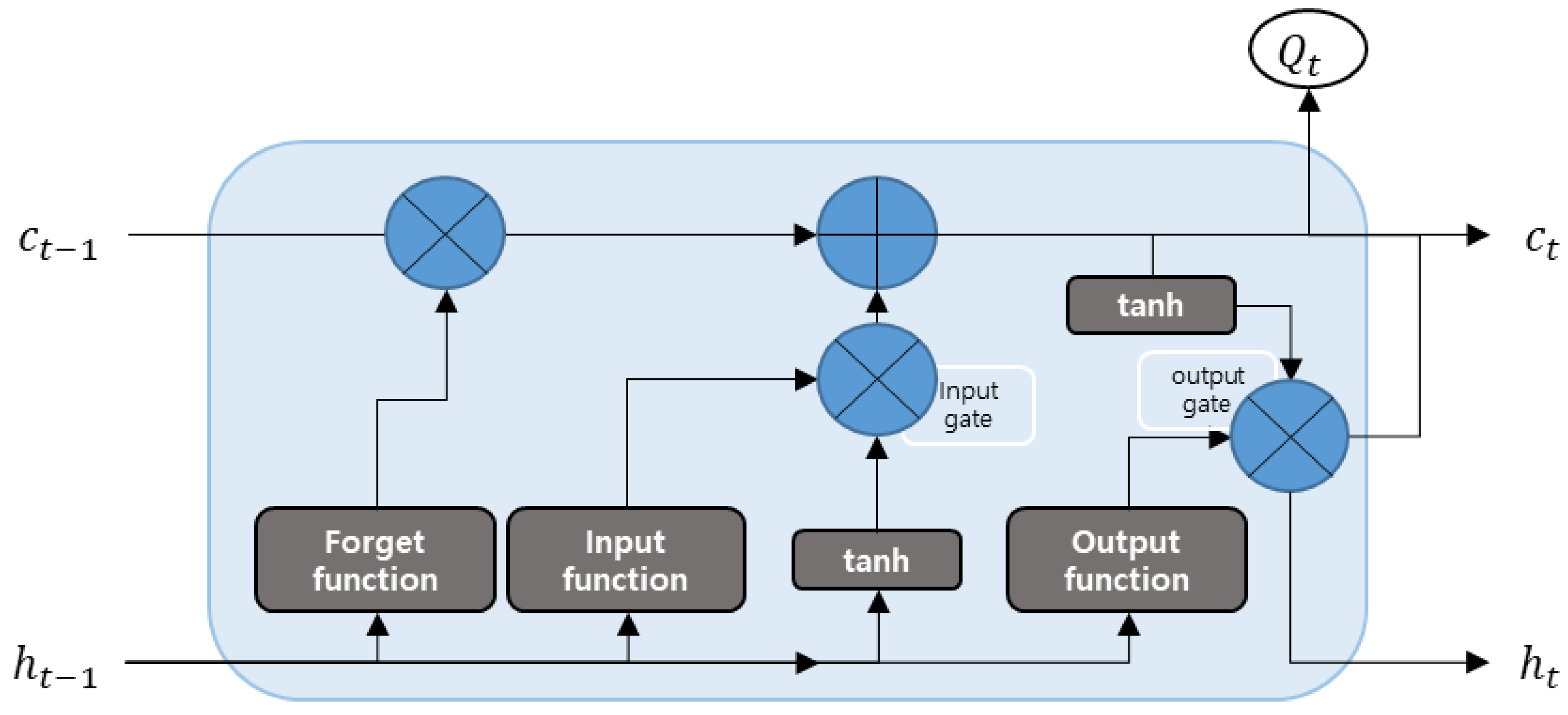
Long short-term memory (LSTM), developed by ameliorating the disadvantages of recurrent neural networks (RNNs), removes unnecessary memories by adding input gates (
), forget gates (
), and output gates (
) to memory cells in the hidden layer [
21,
23,
24,
25], erasing and deciding what to remember. These three gates have a sigmoid function in common. After passing the sigmoid function, a value between 0 and 1 comes out, and the gate is adjusted with these values. In summary, LSTM has a slightly more complex formula for calculating the hidden state than RNNs and adds a value called cell state. Compared to RNNs, LSTM shows excellent performance in processing long sequences of inputs (
Figure 3).
2.4. Deep Neural Network
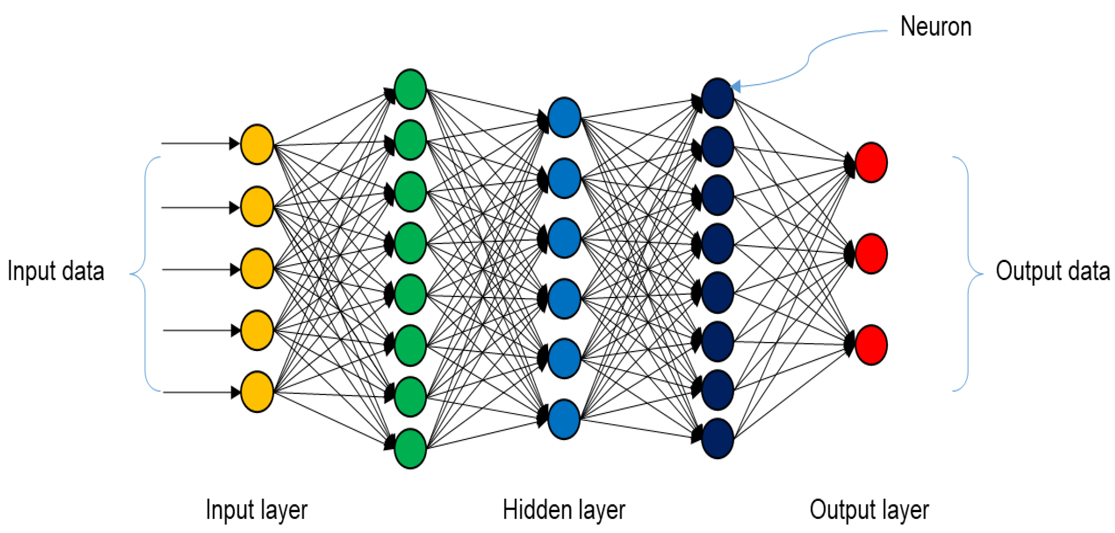
A deep neural network (DNN) is an artificial neural network (ANN) composed of several hidden layers between an input layer and an output layer. DNNs, like regular ANNs, can model complex non-linear relationships. DNNs have the advantage of being able to model complex data with fewer units (nodes) than similarly performed ANNs [
21,
25,
26,
27,
28]. The DNN is trained using a standard-error backpropagation algorithm, and the weights are updated through stochastic gradient descent. Deep neural networks are vulnerable to overfitting because the added layers allow modeling of rare dependencies in the training data. To overcome overfitting, dropout regularization has emerged as one of the regularization methods. In dropout regularization, some units of the hidden layers are randomly omitted during training. This method helps to solve rare dependencies that may occur in the training data (
Figure 4).
2.5. Probability Density Function and Cumulative Distribution Function
The law of probability is the basis for statistical characterization of repeated observations. The probability
of a specific event
is defined as the frequency at which the event will occur at the end of repeated trals [
29,
30,
31].
where
is the frequency of the event
,
is the number of attempts and is a sufficiently large value, and
is called the relative frequency or probability.
Both continuous and discrete random variables are characterized by the probability distribution of a specific value of each variable. The probability density function (PDF) is a function representing the distribution of a random variable. For the probability density function
and the interval
, the probability
that the random variable
is included in the interval is as follows.
A cumulative distribution function (CDF) is a function that gives the probability that a given random variable is less than or equal to a certain value. That is, the cumulative distribution function
means the probability that a certain variable
is not larger than a specific variable
.
Therefore, is a function that increases from 0 to 1 and divides into each class interval to indicate the data belonging to each interval.
2.6. Decision Tree
Decision tree (DT) is a model that derives rules to subdivide similar data and classify them by category by expressing data in a tree-like graph based on the rules of the data [
22,
32,
33,
34,
35]. DT is based on the downward induction method of dynamic programming, and the data separated from the upper node are subdivided into similar data by criteria. And, through iterative subdivision, it is repeated until the final classification by yield is completed. A decision tree consists of a root node, internal nodes, leaf nodes, and branches. Here, in all nodes except the end node, prediction results are derived by learning cases that are satisfied and unsatisfied through conditions based on classification criteria. Depending on the degree of pruning in the learning process of the model, prediction results can be built more accurately. The complexity parameter (Cp) determines the number of trees at which the error rate is lowest. That is, the accuracy of each parameter is identified for pruning, and the prediction result can be expressed based on the optimal parameter (
Figure 5).
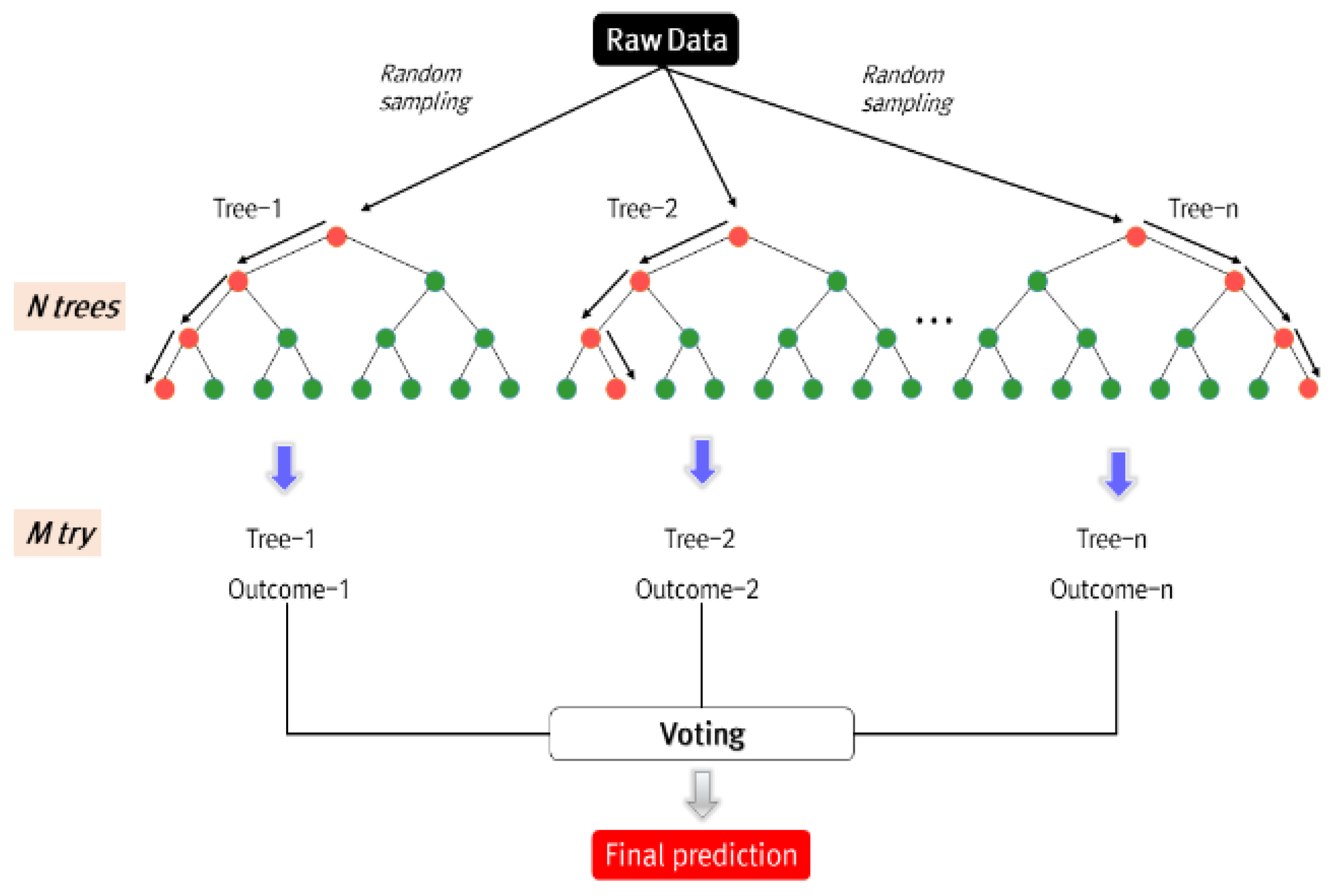
2.7. Random Forest
Random forest (RF) is an ensemble-based model and a classification model that adds voluntariness and the basic principle of bootstrap aggregation (bagging), which is a method of aggregating samples by learning bootstrap models several times in multiple decision tree models. Random forest has high accuracy among classification models [
22,
36,
37,
38,
39]. Random forest randomly extracts learning data based on the basic principle of bagging, independently constructs a decision tree, and generates a total of n-trees. Here, when deriving the output result, the decision tree is randomly determined so that the result can be derived. This is defined as the number of classifiers (mtry). In the learning process, the model is repeatedly trained to select the optimal parameters and derive the best prediction results (
Figure 6).
2.8. Evaluating the Predictive Power of the Model
Correlation analysis, which indicates the correlation between the observed data being measured at the station and the data predicted through the prediction model, is a method designed to quantitatively identify the relationship between two variables [
21,
25,
40].
where, in order to calculate the correlation, first, the deviations of
and
, that is,
and
for each
and
are calculated.
The square error divided by n is the mean square error (
MSE), and the square root of the error is the root mean square error (
RMSE). This is the normalized root mean square error (
NRMSE), which standardizes mean square error and root mean square error [
21,
25,
40,
41].
where
means the
-th actual value and
means the
-th simulated value.
The accuracy verification of the classification model is performed based on the confusion matrix (
Table 2). The confusion matrix is true positive (TP) when an observed value is predicted as 1 and the model result is 1, false negative (FN) when the observed value is predicted as 1 and the model result is 0, and the observed value is 0. Predicting the model output value as 1 is called false positive (FP), and when the observed value is 0, predicting the model output value as 0 is called true negative (TN) [
6,
15,
39].
Based on the calculated confusion matrix, accuracy, error rate, sensitivity, precision, and specificity can be calculated. The F1-score can be calculated as follows using precision and sensitivity, and
is generally marked as 1.
3. Results
3.1. Development of Water Demand Prediction Model Using DNN and LSTM Models
To effectively perform DNN model learning, we determined the optimal combination of learning rate, hidden layers, hidden nodes, optimizer, and activation for the prediction model. Similarly, to effectively perform LSTM model learning, we determined the optimal combination of activation, learning rate, epochs, optimizer, and loss for the prediction model. Additionally, by applying K-fold cross-validation to the dataset during the learning period, we observed an improvement in accuracy for a small dataset (
Table 3).
Table 4 shows the results of the evaluation of predictive power in the evaluation period from 2016 to 2021. The CC of the DNN model is 0.89 and the NRMSE is 12.42. The CC of the LSTM model is 0.95 and the NRMSE is 8.38.
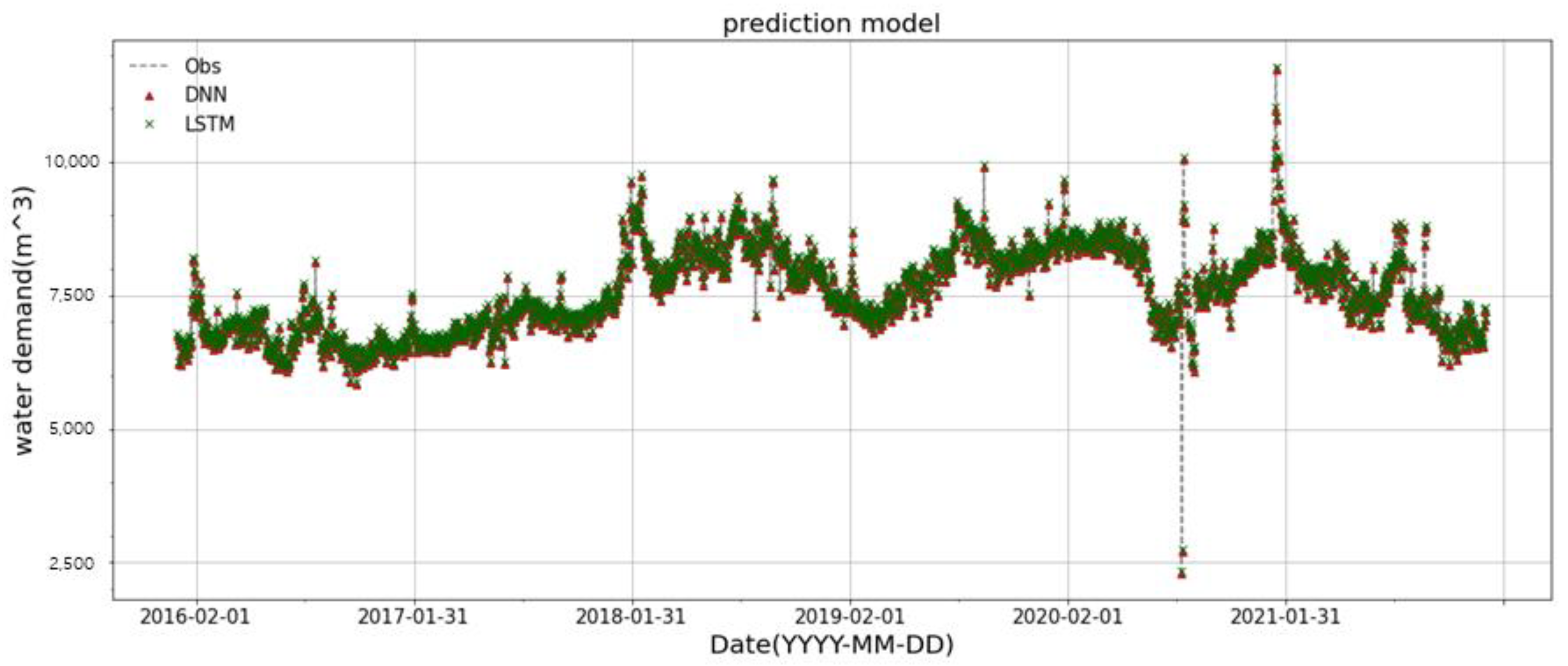
Figure 7 displays the water demand forecasted by the DNN and LSTM models, as well as the actual observed data at the Gurye intake station. The DNN model predicts the overall tendency of water damage well. However, the accuracy of predicting peak values, which are important in prediction, is low. On the other hand, the LSTM model performs better than the DNN model. It not only captures the overall water demand amount and variability well but also accurately predicts the time when the peak value occurs. In forecasting, it is important to predict the overall amount, but it is also important to determine how accurately the highest and lowest points and the peak values for each section are predicted.
Python-based software 3.12 was used, and the processing time was determined quickly within 30 min. A well-designed AI infrastructure leverages high-performance computing capabilities, such as GPUs or TPUs, to perform complex calculations in parallel. This allows machine learning algorithms to process enormous datasets swiftly, leading to faster model training and inference.
3.2. Setting of Crisis Alert Standards
The types of crises considered in managing drought situations include crop damage, a reduction in river maintenance flow, and groundwater depletion due to the shortage of domestic, agricultural, and industrial water. The development of these crises occurs in stages. The first stage is drought caused by a lack of precipitation due to climate change. The second stage is a shortage of domestic, agricultural, and industrial water, along with crop damage in some areas. The third stage involves the expansion of shortages in domestic, agricultural, and industrial water, as well as crop damage, to large-scale areas.
According to drought forecasting and warning standards, the criteria for attention (blue), caution (yellow), alert (orange), and serious (red) are as follows: The attention stage is reached when the water level of the river and water resource facility is lower than normal, necessitating preparation for drought in terms of domestic and industrial water. The caution stage is reached when the river maintenance flow is insufficient, or the dam (reservoir) needs to restrict the supply of water for river maintenance. In the alert stage, it becomes necessary to limit water supply due to the occurrence or anticipation of a partial shortage of domestic and industrial water. The serious stage is reached when the shortage of domestic and industrial water has expanded, and supply restrictions have occurred or are necessary in rivers and dams (reservoirs). Regarding domestic and industrial water, no quantitative risk warning standard has been set, so restrictions on actions at each stage are based on qualitative judgment.
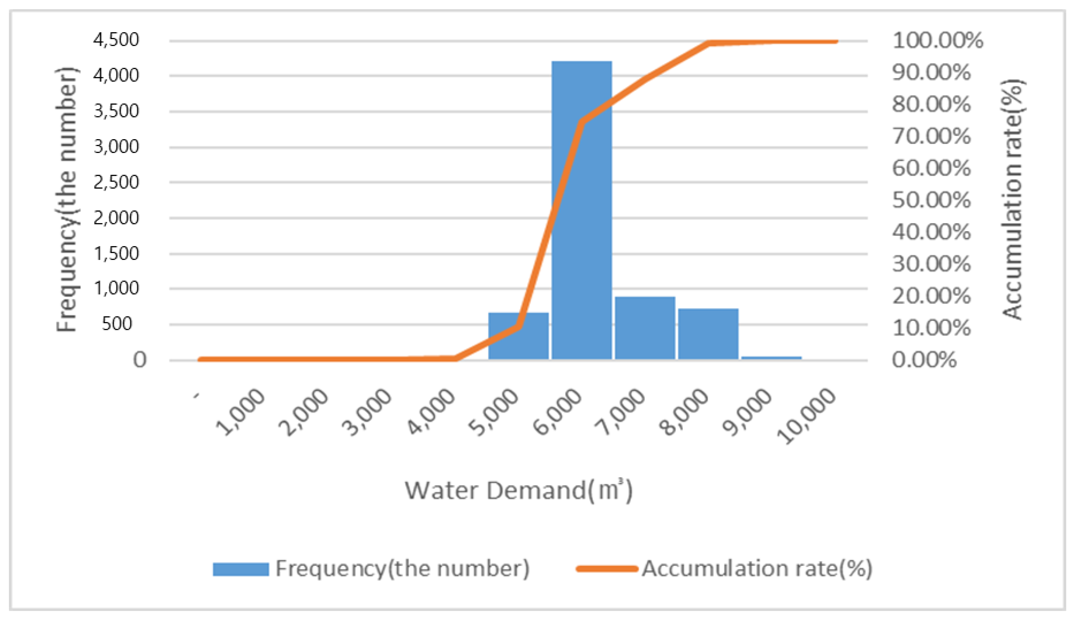
To establish a quantitative standard, a histogram was created to analyze the distribution of water demand data from the Gurye intake station between 2004 and 2021. The water demand at the Gurye intake station increased from 5000 to 6000, with the highest distribution of water demand being between 6000 and 7000 (
Table 5,
Figure 8).
According to the Guidelines for Comprehensive Water Demand Management Plan, the demand for water for living, industrial, and agricultural use is calculated based on 70% to 80% of the maximum daily water supply, which is determined by facility standards. The permitted amount for the Gurye intake station is 9098 (m3/day), which means 70% of the maximum daily water supply is 6368.6 (m3/day), and 80% is 7278.4 (m3/day).
In this study, the crisis warning standards for the Gurye intake station were established by referring to the drought forecasting and warning standards, the Guidelines for Comprehensive Water Demand Management Plan, and previous studies. Taking into account the permitted amount of the Gurye intake station and the maximum water supply per day, the standard for the serious level was set based on the maximum permitted amount of the Gurye intake station, with a standard value of 9098.0 (m
3/day). The standard for the alert stage was set at 75% of the daily maximum water supply, with a standard value of 6823.5 (m
3/day). The caution level was based on 50%, with a standard value of 4549.0 (m
3/day), and the attention level was based on 25%, with a reference value of 2274.5 (m
3/day). The crisis alert standards established in this study are presented in
Table 6 below.
3.3. Development of Water Demand Class Interval Classification Prediction Model
Classification is the process of predicting the dependent variable (class interval) that has the highest correlation with the independent variable. It is a method used to identify the class interval to which the data on water demand samples belong. Classification models can be divided into two categories. The first is the discriminant function model, which determines decision boundaries that divide data into different areas according to class intervals and calculates which intervals are distributed from these decision boundaries. The second is the stochastic model, which calculates the probability of distribution in the class interval for the input data. In this study, the DT and RF models were used to determine the scale of water demand in the near future.
The water demand at the Gurye intake station is affected by the water demand from the previous day, as well as the rainfall, maximum temperature, and average temperature of the surrounding rainfall stations. Taking these factors into account, we collected daily data on the observed water demand at the Gurye intake station and the rainfall, maximum temperature, and average temperature from the previous day at the rainfall stations from 2004 to 2021.
During the learning period, we applied K-fold cross-validation to 4383 data points from 2004 to 2015 and performed model learning and evaluation. Additionally, we used 2192 data points from 2016 to 2021 as the verification interval to assess the accuracy of the model. The DT model learns using one parameter, cp, which represents a parameter for tree pruning of the DT model. Tree pruning is a process that reduces overfitting of the DT and increases its generalizability. The results of the DT model according to the parameters are shown in
Table 7, and we developed the model by selecting the optimal parameters.
Table 8 and
Table 9 show the results of the water demand class interval model during the learning period using the DT model. The parameters of the DT model were optimized based on the input data, and we evaluated the predictive performance of the model.
Table 8 and
Table 9 also show the results of the evaluation period for the water demand class interval classification model using the DT model (
Figure 9).
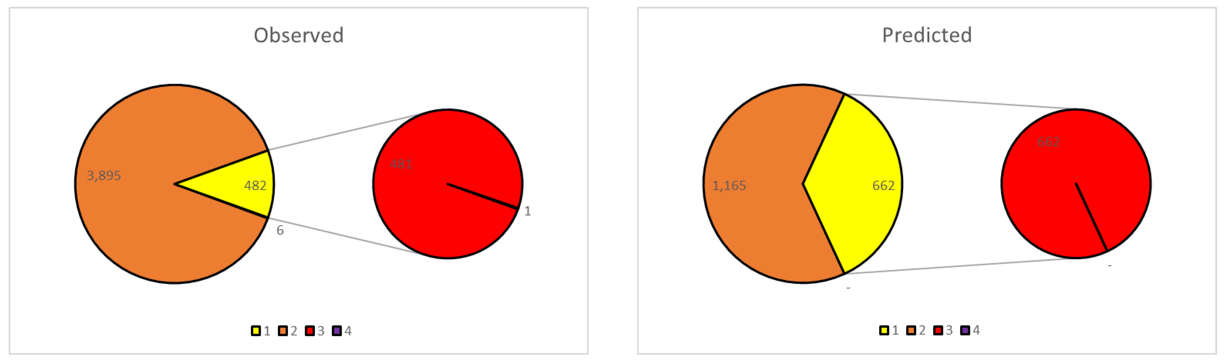
When examining the confusion matrix, we observed that Class 1, Class 2, Class 3, and Class 4 had low predictive power. Overall, the predictive power for all classes was found to be low, with an F1-score of 0.43 (
Table 10).
To determine the learning period, we performed learning and evaluation using K-fold cross-validation on 4383 data points from 2004 to 2015. Additionally, we used 2192 data points from 2016 to 2021 as the verification interval to assess the model’s accuracy. The RF model learns using a single parameter, mtry, which represents a candidate variable to be used in each tree among independent variables.
Table 11 shows the results obtained with different parameters of the RF model. The optimal parameters were selected to develop the model.
Table 12 and
Table 13 present the results of the water demand class intervals model’s learning and evaluation intervals using the RF model. We optimized the parameters of the RF model based on the input data and evaluated the model’s predictive performance. Specifically,
Table 12 shows the results of the learning interval, while
Table 13 displays the evaluation interval of the water demand class interval classification model using the RF model (
Figure 10).
Upon examining the confusion matrix, we found that Class 2, Class 3, and Class 4 exhibited high predictive power. Based on the predictive power evaluation for all classes, we observed that the F1-score was 0.88, indicating high predictive power (
Table 14).
4. Discussion
Water demand forecasting can help reduce the cost of maintaining adequate water supplies. With accurate forecasts, water providers can efficiently manage operations and supply quality water to consumers at a lower cost. When dealing with time-series forecasting problems, it is important to consider the characteristics of both linear and nonlinear models. Linear models can only recognize linear patterns in time-series data, whereas nonlinear models can accurately identify nonlinear relationships in time-series data. This highlights the importance of selecting appropriate input data and constructing a model that considers various situations rather than relying on fixed parameters [
6,
12,
13,
14,
15].
Using AI to predict water demand is an efficient method that relies on accumulated hydrological and meteorological data, especially in areas where obtaining data is difficult. However, models that use large input data or fixed parameters can face various problems and limitations that reduce their predictive power. Linear models, in particular, do not perform well with nonlinear data. Research has shown that AI-based predictive models can overcome these limitations and improve performance. Maximizing the strengths of each model and reducing errors caused by inappropriate input data can lead to more accurate results [
10,
19,
20,
21].
Predicting the scale of water demand in the near future is crucial for permanently expanding water supply and resolving demand management issues to reduce uncertainty. This requires approaching crisis management and implementing adaptive drought measures. At the risk management level, water demand management involves taking appropriate measures to prevent, prepare for, and respond to drought based on an understanding of drought forecasting and warning standards. Early warning to identify risks is crucial, and improving forecasting and warning capabilities should be a priority.
Drought forecasting and warning standards are currently established for weather drought (Meteorological Administration), water for living and industrial use (Ministry of Environment), and water for agriculture (Ministry of Agriculture, Food, and Livestock). Because weather forecasting and warning standards for drought and agricultural water are presented quantitatively, implementing step-by-step national action plans based on this information can be carried out with little uncertainty. However, the standard for forecasting and warning drought for living and industrial water has not been presented quantitatively, leading to relatively high uncertainty in implementing step-by-step national action guidelines based on qualitative judgment.
Water demand adaptive management involves driving near-future information through an iterative learning process in the presence of uncertainty. In this study, supply measures and demand management policies are approached at the level of adaptive management, and information is provided in advance to carry out management measures based on the best information with high speed and accuracy. Flexibility and promptness must be secured in the process of forming and implementing policies by utilizing this information.
5. Conclusions
Drought has serious social and environmental impacts, but it is widespread and occurs gradually. Accordingly, in order to prepare for and respond in advance to damage caused by drought, it is necessary to establish non-structural measures that can be applied flexibly according to the drought stage [
1,
2,
3]. Therefore, in this study, an AI model was applied to predict water demand in real time. Model accuracy was evaluated using data, with the LSTM model achieving a CC of 0.95 and an NRMSE of 8.38, indicating excellent performance [
3,
4,
5,
6,
7,
10,
22].
And standards for each stage of crisis warning were set. AI-based classification models, namely DT and RF models, were used to identify the scale of water demand based on the established standards. The water demand at the Gurye intake station is influenced by the water demand from the day before, and the accuracy of the model was evaluated by considering this influence. As a result of evaluating the accuracy of the model, the F1-score value of the RF model was 0.81, showing excellent performance.
Because water demand prediction is essential for optimal water resource management, many studies have applied and developed various methods for accurate prediction. However, rather than predicting the strategic value of water demand, research is needed to determine how much water demand is insufficient or sufficient in the short term.
Adaptive water demand management can be said to promote information about the near future through an iterative learning process in situations where uncertainty exists. This study focuses on supply and demand management policies and approaches them from an adaptive management perspective, providing advance information so that management measures can be carried out based on the best information quickly and accurately. This information should be utilized to ensure flexibility and speed in the process of policy formulation and implementation.
Author Contributions
Conceptualization, D.K.; Data curation, D.K.; Formal analysis, D.K. and H.N.; Investigation, D.K. and H.N.; Methodology, S.K. and S.C.; Project administration, H.N.; Resources, D.K. and H.N.; Software, D.K., S.K. and S.C.; Supervision, H.N.; Validation, D.K., S.K. and S.C.; Visualization, D.K. and H.N.; Writing—original draft, S.K. and S.C.; Writing—review and editing, H.N. All authors have read and agreed to the published version of the manuscript.
Funding
This work was supported by the Korea Environment Industry & Technology Institute (KEITI) through the Water Management Program for Drought (or Project), funded by Korea’s Ministry of Environment (MOE) (2022003610004).
Data Availability Statement
The data presented in this study are available on request from the corresponding author. The data are not publicly available because they relate to real commercial cases.
Conflicts of Interest
The authors declare no conflict of interest.
References
- Farhan, S.L.; Abdelmonem, M.G.; Nasar, Z.A. The urban transformation of traditional city centres: Holy Karbala as a case study. ArchNet-IJAR: Int. J. Archit. Res. 2018, 12, 53. [Google Scholar] [CrossRef]
- Banihabib, M.E.; Mousavi-Mirkalaei, P. Extended linear and non-linear auto-regressive models for forecasting the urban water consumption of a fast-growing city in an arid region. Sustain. Cities Soc. 2019, 48, 101585. [Google Scholar] [CrossRef]
- Jeong, G.; Kang, D.; Kim, T. Evaluation of hydropower dam water supply capacity (III): Development and application of drought operation rule for hydropower dams in Han river. J. Korea Water Resour. Assoc. 2022, 55, 531–543. [Google Scholar] [CrossRef]
- Zubaidi, S.L.; Kot, P.; Hashim, K.; Alkhaddar, R.; Abdellatif, M.; Muhsin, Y.R. Using LARS–WG model for prediction of temperature in Columbia City, USA. IOP Conf. Ser. Mater. Sci. Eng. 2019, 584, 012026. [Google Scholar] [CrossRef]
- Hashim, K.S.; Al-Saati, N.H.; Alquzweeni, S.S.; Zubaidi, S.L.; Kot, P.; Kraidi, L.; Hussein, A.; Alkhaddar, R.; Shaw, A.; Alwash, R. Decolourization of dye solutions by electrocoagulation: An investigation of the effect of operational parameters. IOP Conf. Ser. Mater. Sci. Eng. 2019, 584, 012024. [Google Scholar] [CrossRef]
- Kim, J.; Kim, D.; Wang, W.; Lee, H.; Lee, M.; Kim, H.S. Comparative analysis of linear model and deep learning algorithm for water usage prediction. J. Korea Water Resour. Assoc. 2021, 54, 1083–1093. [Google Scholar] [CrossRef]
- Jang, O.J.; Moon, Y.I.; Moon, H.T. Methodology for assessment and forecast of drought severity based on the water balance analysis. J. Korea Water Resour. Assoc. 2021, 54, 241–254. [Google Scholar] [CrossRef]
- Msiza, I.S.; Nelwamondo, F.V.; Marwala, T. Water demand forecasting using multi-layer perceptron and radial basis functions. In Proceedings of the 2007 International Joint Conference on Neural Networks, Orlando, FL, USA, 12–17 August 2007; pp. 13–18. [Google Scholar] [CrossRef]
- Global Water Intelligence; Yearbook IDA; Global Water Summit; Rate Card. Global Water Intelligence; Global Water Intelligence: Oxford, UK, 2011; Volume 12, pp. 1–72. [Google Scholar]
- Kwon, H.H.; Kim, M.J.; Kim, O.G. A development of water demand forecasting model based on Wavelet transform and Support vector machine. J. Korea Water Resour. Assoc. 2012, 45, 1187–1199. [Google Scholar] [CrossRef]
- Kusangaya, S.; Toucher, M.L.W.; van Garderen, E.A. Evaluation of uncertainty in capturing the spatial variability and magnitudes of extreme hydrological events for the uMngeni catchment, South Africa. J. Hydrol. 2018, 557, 931–946. [Google Scholar] [CrossRef]
- Koo, J.Y.; Yu, M.J.; Kim, S.G.; Shim, M.H.; Akira, K. Estimation of long-term water demand by principal component and cluster analysis and practical application. J. Korean Soc. Environ. Eng. 2005, 27, 870–876. [Google Scholar]
- Atsalakis, G.; Minoudaki, C. Daily irrigation water demand prediction using Adaptive Neuro-Fuzzy Inferences Systems (ANFIS). In Proceedings of the 3rd IASME/WSEAS International Conference on Energy, Environment, Ecosystems and Sustainable Development (EEESD’07), Agios Nikolaos, Crete Island, Greece, 24–26 July 2007; World Scientific and Engineering Academy and Society Press (WSEAS Press): Athens, Greece, 2007; pp. 368–373. [Google Scholar]
- Alvisi, S.; Franchini, M.; Marinelli, A. A short-term, pattern-based model for water-demand forecasting. J. Hydroinform. 2007, 9, 39–50. [Google Scholar] [CrossRef]
- Lee, H.; Kim, H.S.; Kim, S.; Kim, D.; Kim, J. Development of a method for urban flooding detection using unstructured data and deep learing. J. Korea Water Resour. Assoc. 2021, 54, 1233–1242. [Google Scholar] [CrossRef]
- Tabesh, M.; Dini, M. Fuzzy and neuro-fuzzy models for short-term water demand forecasting in Tehran. Iran. J. Sci. Technol. Trans. B Eng. 2009, 33, 61–77. [Google Scholar]
- Choi, G.S.; Yu, C.; Jin, R.M.; Yu, S.K.; Chun, M.G. Short-term water demand forecasting algorithm using AR model and MLP. J. Korean Inst. Intell. Syst. 2009, 19, 713–719. [Google Scholar] [CrossRef]
- Firat, M.; Turan, M.E.; Yurdusev, M.A. Comparative analysis of neural network techniques for predicting water consumption time series. J. Hydrol. 2010, 384, 46–51. [Google Scholar] [CrossRef]
- Altunkaynak, A.; Nigussie, T.A. Monthly water consumption prediction using season algorithm and wavelet transform–based models. J. Water Resour. Plan. Manag. 2017, 143, 04017011. [Google Scholar] [CrossRef]
- Choi, J.; Kim, J. Analysis of water consumption data from smart water meter using machine learning and deep learning algorithms. J. Inst. Electron. Inf. Eng. 2018, 55, 31–39. [Google Scholar]
- Kim, D.; Lee, J.; Kim, J.; Lee, M.; Wang, W.; Kim, H.S. Comparative analysis of long short-term memory and storage function model for flood water level forecasting of Bokha stream in NamHan River, Korea. J. Hydrol. 2022, 606, 127415. [Google Scholar] [CrossRef]
- Kim, D.; Lee, K.; Hwang-Bo, J.; Kim, H.S.; Kim, S. Development of the Method for Flood Water Level Forecasting and Flood Damage Warning Using an AI-based Model. J. Korean Soc. Hazard Mitig. 2022, 22, 145–156. [Google Scholar] [CrossRef]
- Hu, C.; Wu, Q.; Li, H.; Jian, S.; Li, N.; Lou, Z. Deep learning with a long short-term memory networks approach for rainfall-runoff simulation. Water 2018, 10, 1543. [Google Scholar] [CrossRef]
- Fan, H.; Jiang, M.; Xu, L.; Zhu, H.; Cheng, J.; Jiang, J. Comparison of long short term memory networks and the hydrological model in runoff simulation. Water 2020, 12, 175. [Google Scholar] [CrossRef]
- Kim, D.; Han, H.; Wang, W.; Kim, H.S. Improvement of Deep Learning Models for River Water Level Prediction Using Complex Network Method. Water 2022, 14, 466. [Google Scholar] [CrossRef]
- Bengio, Y. Learning Deep Architectures for AI. Found. Trends® Mach. Learn. 2009, 2, 1–127. [Google Scholar] [CrossRef]
- Szegedy, C.; Toshev, A.; Erhan, D. Deep neural networks for object detection. Adv. Neural Inf. Process. Syst. 2013, 26. [Google Scholar]
- Schmidhuber, J. Deep learning in neural networks: An overview. Neural Netw. 2015, 61, 85–117. [Google Scholar] [CrossRef]
- Alzaatreh, A.; Lee, C.; Famoye, F. A new method for generating families of continuous distributions. Metron 2013, 71, 63–79. [Google Scholar] [CrossRef]
- Al-Zahrani, B.; Al-Sobhi, M. On parameters estimation of Lomax distribution under general progressive censoring. J. Qual. Reliab. Eng. 2013, 2013, 431541. [Google Scholar] [CrossRef]
- Rao, R.S.; Durgamamba, A.N.; Ravikumar, M.; Kantam, R. Discriminating between size biased Lomax distribution and Pareto-Rayleigh distribution. Open J. Appl. Theor. Math. 2016, 2, 409–418. [Google Scholar]
- Quinlan, J.R. Simplifying decision trees. Int. J. Man-Mach. Stud. 1987, 27, 221–234. [Google Scholar] [CrossRef]
- Song, Y.S.; Chae, B.G. Development to Prediction Technique of Slope Hazards in Gneiss Area using Decision Tree Model. J. Eng. Geol. 2008, 18, 45–54. [Google Scholar]
- Breiman, L.; Friedman, J.H.; Olshen, R.A.; Stone, C.J. Classification and Regression Trees; Routledge: London, UK, 2017. [Google Scholar] [CrossRef]
- Choi, C.; Kim, J.; Kim, D.; Lee, J.; Kim, D.; Kim, H.S. Development of heavy rain damage prediction functions in the seoul capital Area using machine learning techniques. J. Korean Soc. Hazard Mitig. 2018, 18, 435–447. [Google Scholar] [CrossRef]
- Breiman, L. Random forests. Mach. Learn. 2001, 45, 5–32. [Google Scholar] [CrossRef]
- Choi, C.K. Evaluation of Flood Impact Variables and Development of Flood Damage Function: Case Study for Residential Buildings and Contents. Ph.D. Thesis, Inha University, Incheon, Republic of Korea, 2017. [Google Scholar]
- Kim, J.; Lee, J.; Kim, D.; Choi, C.; Lee, M.; Kim, H.S. Developing a Prediction Model (Heavy Rain Damage Occurrence Probability) Based on Machine Learning. J. Korean Soc. Hazard Mitig. 2019, 19, 115–127. [Google Scholar] [CrossRef]
- Alali, Y.; Harrou, F.; Sun, Y. Unlocking the Potential of Wastewater Treatment: Machine Learning Based Energy Consumption Prediction. Water 2023, 15, 2349. [Google Scholar] [CrossRef]
- Kim, D.; Han, H.; Wang, W.; Kang, Y.; Lee, H.; Kim, H.S. Application of deep learning models and network method for comprehensive air-quality index prediction. Appl. Sci. 2022, 12, 6699. [Google Scholar] [CrossRef]
- Fawcett, T. An introduction to ROC analysis. Pattern Recognit. Lett. 2006, 27, 861–874. [Google Scholar] [CrossRef]
Figure 1.
The location of Gurye intake station in the Seomjin river basin [
3,
6,
10].
Figure 1.
The location of Gurye intake station in the Seomjin river basin [
3,
6,
10].
Figure 2.
Conceptual diagram of a study on developing an AI−based water demand prediction and classification model for Gurye intake station.
Figure 2.
Conceptual diagram of a study on developing an AI−based water demand prediction and classification model for Gurye intake station.
Figure 3.
The structure of long short-term memory [
21,
23,
24,
25].
Figure 3.
The structure of long short-term memory [
21,
23,
24,
25].
Figure 4.
The structure of a deep neural network [
21,
25,
26,
27,
28].
Figure 4.
The structure of a deep neural network [
21,
25,
26,
27,
28].
Figure 5.
The structure of decision tree [
22,
32,
33,
34,
35].
Figure 5.
The structure of decision tree [
22,
32,
33,
34,
35].
Figure 6.
The structure of random forest [
22,
36,
37,
38].
Figure 6.
The structure of random forest [
22,
36,
37,
38].
Figure 7.
Observed (Gurye intake station; water demand) and predicted water demand prediction model from DNN and LSTM models. Red triangle represents DNN model. Green X represents LSTM model.
Figure 7.
Observed (Gurye intake station; water demand) and predicted water demand prediction model from DNN and LSTM models. Red triangle represents DNN model. Green X represents LSTM model.
Figure 8.
Histogram of water intake data.
Figure 8.
Histogram of water intake data.
Figure 9.
Comparison with prediction results and observation results using DT.
Figure 9.
Comparison with prediction results and observation results using DT.
Figure 10.
Comparison with prediction results and observation results using RF.
Figure 10.
Comparison with prediction results and observation results using RF.
Table 1.
Basic statistics for the dependent and independent variables.
Table 1.
Basic statistics for the dependent and independent variables.
| Variable | Max | Min | Mean | Standard Deviation |
|---|
| Water demand (m3) | 11,806.00 | 2343.00 | 6781.29 | 807.24 |
| Average temperature (°C) | 31.10 | −10.10 | 13.45 | 9.71 |
| Minimum temperature (°C) | 28.80 | −14.80 | 8.04 | 10.29 |
| Maximum temperature (°C) | 38.30 | −8.30 | 20.02 | 9.94 |
| Average wind speed (m/s) | 26.60 | 0.00 | 7.09 | 2.72 |
| Daily precipitation (mm) | 7.80 | 0.00 | 1.44 | 0.82 |
Table 2.
The structure of the confusion matrix.
Table 2.
The structure of the confusion matrix.
| Classification | Predicted |
|---|
| Negative | Positive |
|---|
| Observed | Negative | True negative (TN) | False positive (FP) |
| Positive | False negative (FN) | True positive (TP) |
Table 3.
Settings of hyper-parameters in DNN and settings of parameters in LSTM.
Table 3.
Settings of hyper-parameters in DNN and settings of parameters in LSTM.
| DNN | LSTM |
|---|
| Hyper-Parameter | Values | Parameter | Values |
|---|
| Learning rate | 0.1 | Activation | ReLU |
| Hidden layer | 3 | Loss | Mean square error |
| Hidden nodes | 4 | Epoch | 53 |
| Optimizer | Adam | Optimizer | Adam |
| Activation | ReLU | Learning rate | 0.1 |
Table 4.
Evaluation of predictive power using CC and NRMSE.
Table 4.
Evaluation of predictive power using CC and NRMSE.
| Classification | CC | NRMSE
(%) |
|---|
| DNN | 0.89 | 12.42 |
| LSTM | 0.95 | 8.38 |
Table 5.
Frequency and accumulation of water demand data.
Table 5.
Frequency and accumulation of water demand data.
Water Demand
() | Frequency
(Number) | Accumulation Rate
(%) |
|---|
| 0 | 0 | 0.00 |
| 1000 | 0 | 0.00 |
| 2000 | 2 | 0.03 |
| 3000 | 2 | 0.06 |
| 4000 | 19 | 0.35 |
| 5000 | 670 | 10.54 |
| 6000 | 4209 | 74.56 |
| 7000 | 891 | 88.11 |
| 8000 | 722 | 99.09 |
| 9000 | 52 | 99.88 |
| 10,000 | 8 | 100.00 |
Table 6.
Setting the crisis alert standards at Gurye intake station.
Table 6.
Setting the crisis alert standards at Gurye intake station.
| Class | Classification | Water Demand
(Number) |
|---|
| Serious | ≤ 11,000.0 | 38 |
| Alert | 6823.50 9097.0 | 2102 |
| Caution | 4549.00 6823.0 | 4313 |
| Attention | 2274.50 4548.0 | 8 |
Table 7.
Derivation of parameters for a decision tree model.
Table 7.
Derivation of parameters for a decision tree model.
| Classification | Cp | Accuracy |
|---|
| 1 | 0.00102 | 0.8920 |
| 2 | 0.00204 | 0.8932 |
| 3 | 0.00512 | 0.8952 |
| 4 | 0.00614 | 0.8953 |
| 5 | 0.05635 | 0.8909 |
Table 8.
Water demand classification prediction model performance evaluation using decision tree (learning section).
Table 8.
Water demand classification prediction model performance evaluation using decision tree (learning section).
| Tree | Obs. |
|---|
| 1 | 2 | 3 | 4 |
|---|
| Pre. | 1 | 0 | 6 | 0 | 0 |
| 2 | 0 | 3767 | 128 | 0 |
| 3 | 0 | 298 | 183 | 0 |
| 4 | 0 | 1 | 0 | 0 |
Table 9.
Water demand classification prediction model performance evaluation using decision tree (evaluation section).
Table 9.
Water demand classification prediction model performance evaluation using decision tree (evaluation section).
| Tree | Obs. |
|---|
| 1 | 2 | 3 | 4 |
|---|
| Pre. | 1 | 0 | 0 | 0 | 0 |
| 2 | 1 | 351 | 801 | 12 |
| 3 | 1 | 23 | 624 | 14 |
| 4 | 0 | 0 | 0 | 0 |
Table 10.
An evaluation of the applicability of a flood damage classification prediction model using decision tree model.
Table 10.
An evaluation of the applicability of a flood damage classification prediction model using decision tree model.
| Class | 1 | 2 | 3 | 4 |
|---|
| Precision | 0.00 | 0.94 | 0.44 | 0.04 |
| Sensitivity | 0.00 | 0.30 | 0.94 | 1.00 |
| F1-score | 0.43 |
Table 11.
Derivation of parameters for a random forest model.
Table 11.
Derivation of parameters for a random forest model.
| Classification | Mtry | Accuracy |
|---|
| 1 | 1 | 0.8991 |
| 2 | 2 | 0.8915 |
| 3 | 3 | 0.8821 |
| 4 | 4 | 0.8785 |
Table 12.
Water demand classification prediction model performance evaluation using random forest (learning section).
Table 12.
Water demand classification prediction model performance evaluation using random forest (learning section).
| Tree | Obs. |
| 1 | 2 | 3 | 4 |
| Pre. | 1 | 2 | 4 | 0 | 0 |
| 2 | 0 | 3823 | 72 | 0 |
| 3 | 0 | 248 | 233 | 0 |
| 4 | 0 | 1 | 0 | 0 |
Table 13.
Water demand classification prediction model performance evaluation using random forest (evaluation section).
Table 13.
Water demand classification prediction model performance evaluation using random forest (evaluation section).
| Tree | Obs. |
|---|
| 1 | 2 | 3 | 4 |
|---|
| Pre. | 1 | 1 | 0 | 0 | 0 |
| 2 | 1 | 782 | 77 | 0 |
| 3 | 0 | 37 | 1246 | 7 |
| 4 | 0 | 0 | 0 | 41 |
Table 14.
An evaluation of the applicability of a flood damage classification prediction model using random forest.
Table 14.
An evaluation of the applicability of a flood damage classification prediction model using random forest.
| Class | 1 | 2 | 3 | 4 |
|---|
| Precision | 0.50 | 0.95 | 0.94 | 0.85 |
| Sensitivity | 1.00 | 0.91 | 0.97 | 1.00 |
| F1-score | 0.88 |
| Disclaimer/Publisher’s Note: The statements, opinions and data contained in all publications are solely those of the individual author(s) and contributor(s) and not of MDPI and/or the editor(s). MDPI and/or the editor(s) disclaim responsibility for any injury to people or property resulting from any ideas, methods, instructions or products referred to in the content. |
© 2023 by the authors. Licensee MDPI, Basel, Switzerland. This article is an open access article distributed under the terms and conditions of the Creative Commons Attribution (CC BY) license (https://creativecommons.org/licenses/by/4.0/).


