Advancing Discharge Ratings: A Novel Approach Based on Observed and Derivable GIS Factors in Alluvial Systems

Abstract

Depth–discharge rating is required at gauged and ungauged locations for hydrologic modeling of alluvial systems to evaluate streamflow and manage regional water resources. Spanning low to high-flow conditions, manual field measurements are used to develop discharge ratings at gauged locations, producing continuous flow data from automated water depth measurements. The discharge rating is dependent on channel geometry, stream slope, vegetation, roughness coefficient, sediment load, and bank stability. To construct discharge ratings for many locations within larger model domains (hundreds to thousands of km²), intensive GIS and manual (spreadsheet) data manipulation are often required. In this analysis, available USGS gauging stations and readily available GIS coverages were used to learn and implement a novel method to characterize the depth–discharge relationships for hydrologic modeling of larger or complex areas using commonly available data and normalization techniques. The improved procedure simply uses drainage area, channel slope, and channel width, readily derivable GIS data, to develop discharge ratings for gauged and ungauged sections. The discharge rating curves for 70 USGS streamflow gauges were reproduced using the procedure. Then, the produced and observed discharge rating curves were compared to evaluate the accuracy of the method. In the analysis of streamflow depth predictions, the average Root Mean Squared Error was recorded at approximately 0.38 m (≈1.24 ft), with an interquartile range between 0.21 m and 0.49 m. The Mean Error remained centered around 0 m, with interquartile values ranging from −0.24 m to 0.24 m.

1. Introduction

Managing water resources is challenging under the impacts of climate change and the ever-increasing demand from global population growth, which also leads to increased urbanization [1]. Managing water resources depends on quantifying the available water resources and understanding the impacts of these and other stresses. In many cases, decisions concerning the best water management practice require using hydrologic simulation models [2]. Hydrologic simulation models simplify complex real-world hydrology and estimate the hydrologic responses to alternative water resource management actions. These models can be used for extended periods of continuous simulation (years) or evaluating single storm event responses [3]. The objective of developing hydrologic models can be to assess changes in streamflow due to changes to input stresses (e.g., climate variability, land use change, diversion options, mining effects, and stream–aquifer interaction from pumping stresses) to provide decision makers with the knowledge that enables better water resources management [4]. Hydrologic models are conceptualized based on the model objectives (questions asked) and available budgets [5].

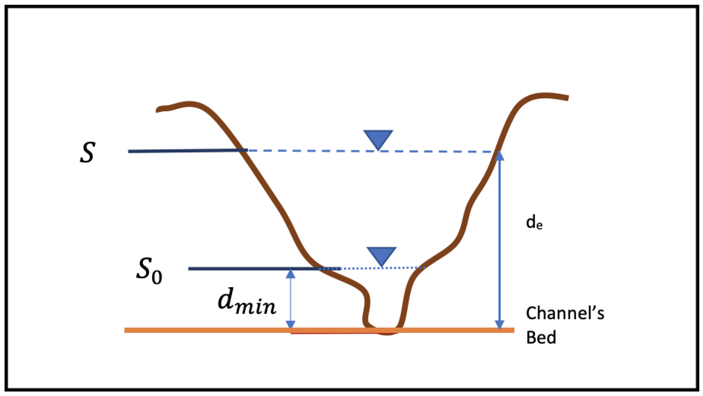
Streamflow discharge is the quantity of water transported through a channel during a specific time, and the stage is the water surface height in a waterbody above a known datum [3]. A depth–discharge relationship or discharge rating is a relationship between the flow rate and stream stage or water depth at a channel outlet [6]. Within a hydrologic model, a discharge rating is required at the outlet of each simulation unit representing a portion of an alluvial wetland/stream system [7]. For example, combined input of stage–discharge storage tabulated discharge rating is required for popular hydrologic models such as HSPF [8] and SWMM [9], as well as many others.

The hydrologic response within a model is very sensitive to discharge rating relationships, and these data are time-consuming for modelers to develop. The discharge rating depends on channel geometry, stream slope, vegetation, roughness coefficient, sediment load, and bank stability [10]. Intensive GIS and manual (spreadsheet) data manipulation is required to construct discharge ratings for a model domain. This is especially problematic when the outlets of most stream reaches (i.e., model simulation units) do not have measured cross-sections, discharge ratings, or continuous discharge records. Moreover, the required work becomes daunting when hydrologic models are required for large areas with extensive alluvial stream and wetland systems.

In most applications, the available data to develop discharge ratings include GIS coverages and a few U.S. Geological Survey (USGS) streamflow gauging stations. The available stage–discharge data most likely originate from USGS stage gauging stations [11]. Generally, USGS stage–discharge rating curves are available at established USGS streamflow measurement stations. However, they are relative to fixed local or National Geodetic Vertical Datum of 1929 (NGVD 29) or North American Vertical Datum of 1988 (NAVD 88) datums and can shift over time [12]. These local or fixed datum stage–discharge rating relationships must be converted to depth–discharge ratings, considered more fixed over time. However, these data only represent one stream cross-section and do little to help populate discharge ratings when a large regional model may possess several hundred or thousands of stream sections that all require discharge ratings [4].

The standard approach to developing a stream’s stage–discharge relationship or discharge rating is to visit the field several times to measure the flow for different stages, covering a series of low-to-high flows [13]. These observations are then used to develop a curve that can convert the continuous stream-stage measurements to discharge estimates [13]. Normally, to build a measured stage–discharge relationship in natural streams, observed stages must be plotted against the observed discharges [14]. Alternatively, empirical methods to build discharge ratings can be used, such as assuming the streamflow is in uniform open channel flow with a prismatic channel section and then using Manning’s or similar equations to predict or calculate flow estimates [3]. These empirical methods require measured or estimated channel properties such as the cross-section area, slope, and subjectively interpreted roughness coefficients [4,13,15]. Channel properties are seldom available online or from GIS databases. They are expensive and time-consuming to obtain, especially for larger regional assessments with hundreds to thousands of stream sections that must be parameterized with discharge rating tables.

Depth–discharge relationships are more consistent than stage–discharge in live beds and vegetated natural sections [6]. They are thus more useful input for the discharge rating of alluvial stream/wetland systems [6]. This study sought to develop a method to characterize the depth–discharge relationship for alluvial channels by using readily available GIS data, building on the work of Mueses et al. [6], Lewelling [16], Emmet [17], and Leopold [18].

As pointed out in the discussion above, discharge rating curves of natural streams tied to a fixed datum are not fixed; they shift over time. The changes in the live-bed channels and floodplains over time result in shifting discharge ratings in natural streams [19]. Vegetation changes, fallen trees, live (variable) bed materials, and anthropogenic activities cause discharge rating curves to shift up or down over time. As a result, discharge rating data tied to the stage will not have a fixed singular one-to-one relationship, and a particular discharge threshold may be experienced for many different stages. Hydrologic models generally require a fixed time, one-to-one (depth–discharge pairs) discharge rating as an input. Mueses et al. 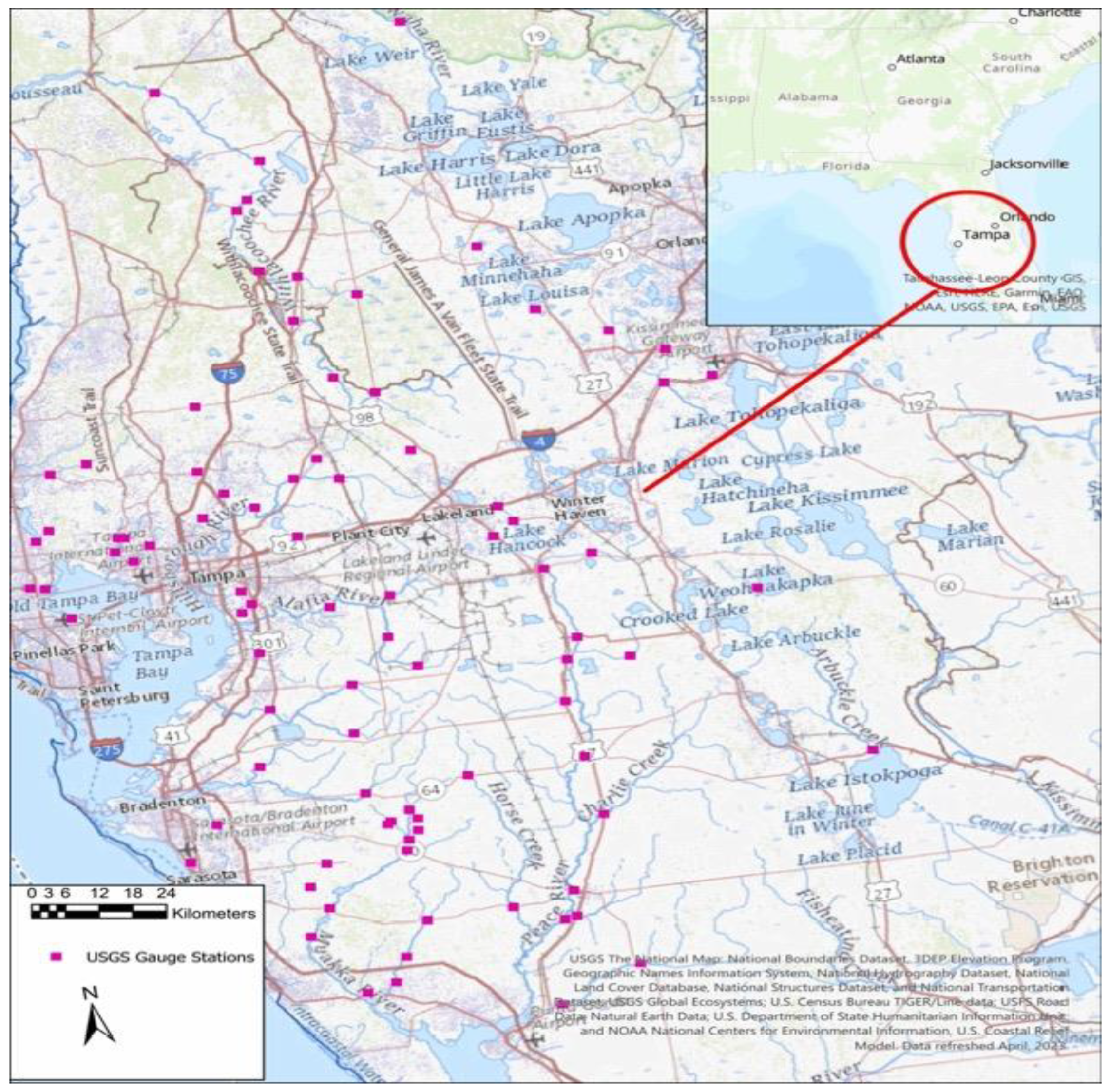[6] developed a simple model to produce an approximated fixed discharge rating curve using readily available GIS data. Mueses et al. [6] used 35 streamflow stations in southwest Florida to reproduce depth–discharge curves by normalizing the daily discharge and depth using the 10% discharge exceedance (Q₁₀), the corresponding depth (d₁₀), and a power law exponent (m_Mueses) to describe rating curve behavior.

In the expected application of the Mueses et al. [6] approach, Q₁₀, d₁₀, and m_Mueses (exponent) values would be derived from GIS data, and the exponents would be found from nearby gauge settings or using average fitted exponents. Using the drainage area to predict Q₁₀ proved to be an efficient approach for predicting that variable. However, it was noted that there would be uncertain outcomes in other areas, and deriving Q₁₀ relationships could be regionally or locally dependent. However, searching for a simplistic method to predict d₁₀ using a similar analysis was not as productive. A method based on the square root of drainage area was hypothesized and tested but resulted in high errors and pore R² (R² ≤ 0.6) in depth prediction. There was another dilemma: how best to estimate the m_Mueses exponent for ungauged sections? When analyzing gauged sites, each site was found to have a different exponent. It is suspected that each site (and thus each reach) possesses a different exponent based on the impact of the channel’s shape, friction, and slope on the discharge rating behavior.

Lewelling [16] discussed one of the fundamentals of streamflow behavior that should be considered in this approach: discharge rating behavior is different for in-channel stages than out-of-bank flows. Generally, flows greater than 10% exceedance flows (less than 10% exceedance) begin to approach out-of-bank flows (flood stage). In comparison, the majority of the discharges (greater than 10% exceedance) are contained within the channel bank in natural and man-made sections [16]. In addition, Leopold et al. [18] introduced the idea of normalizing the depth and discharge using the bankfull values to create a regional dimensionless depth–discharge relationship for ungauged locations. According to Mueses et al. [6], when their approach was compared to USGS observations, the results generally presented only small errors for intermediate and low discharges, with generally larger errors reserved for high (and presumably more out-of-bank) discharges.

It is well-recognized that natural channels exhibit different flow behavior (control) with characteristically different frictional conditions and geometries for in-bank and out-of-bank flows [18]. Thus, each control phase would exhibit different discharge rating behavior, especially the transition from channel control to floodplain control. Therefore, using a single exponent (m_Mueses-value) to reproduce the depth–discharge curve for low and extreme discharges may be expected to yield relatively higher errors for extreme discharges, which was the hypothesized reason for the relatively high errors in larger flows in Mueses et al. [6].

Alluvial wetlands are those floodplain-type wetlands that encompass (surround) the main channel (thalweg), the storage of which greatly affects the out-of-bank flows through storage attenuation and differing floodplain frictional conditions [20]. Alluvial wetlands, therefore, have incised channels representing the main thalweg and/or subchannels or branches in a dendritic stream system [21]. These wetland channels are formed naturally and are in relation (proportion) to the dominant discharges strongly controlled by the cumulative drainage area, upland, and climatologic factors (e.g., soil types and mean annual rainfall). Thus, the channel size naturally increases with the high flow discharge index (e.g., Q₁₀) [17]. Consequently, natural streams seem to achieve a balance between the channel geometry and the conveyance of the periodic but infrequent larger flows experienced in the channel [3].

Lawlor [22] investigated the relationship between the bankfull discharge, drainage area, and channel morphology to estimate the bankfull discharge at ungauged stations. The results showed that relating the drainage area to channel morphologic characteristics and the drainage area to the bankfull discharge using regression analysis can be useful to approximate channel morphology and/or bankfull discharge [22]. Based on the findings of [17,23], the size of the drainage area within the same region can be reliably used to determine the bankfull channel discharge, bankfull mean depth, bankfull width, and bankfull cross-section area.

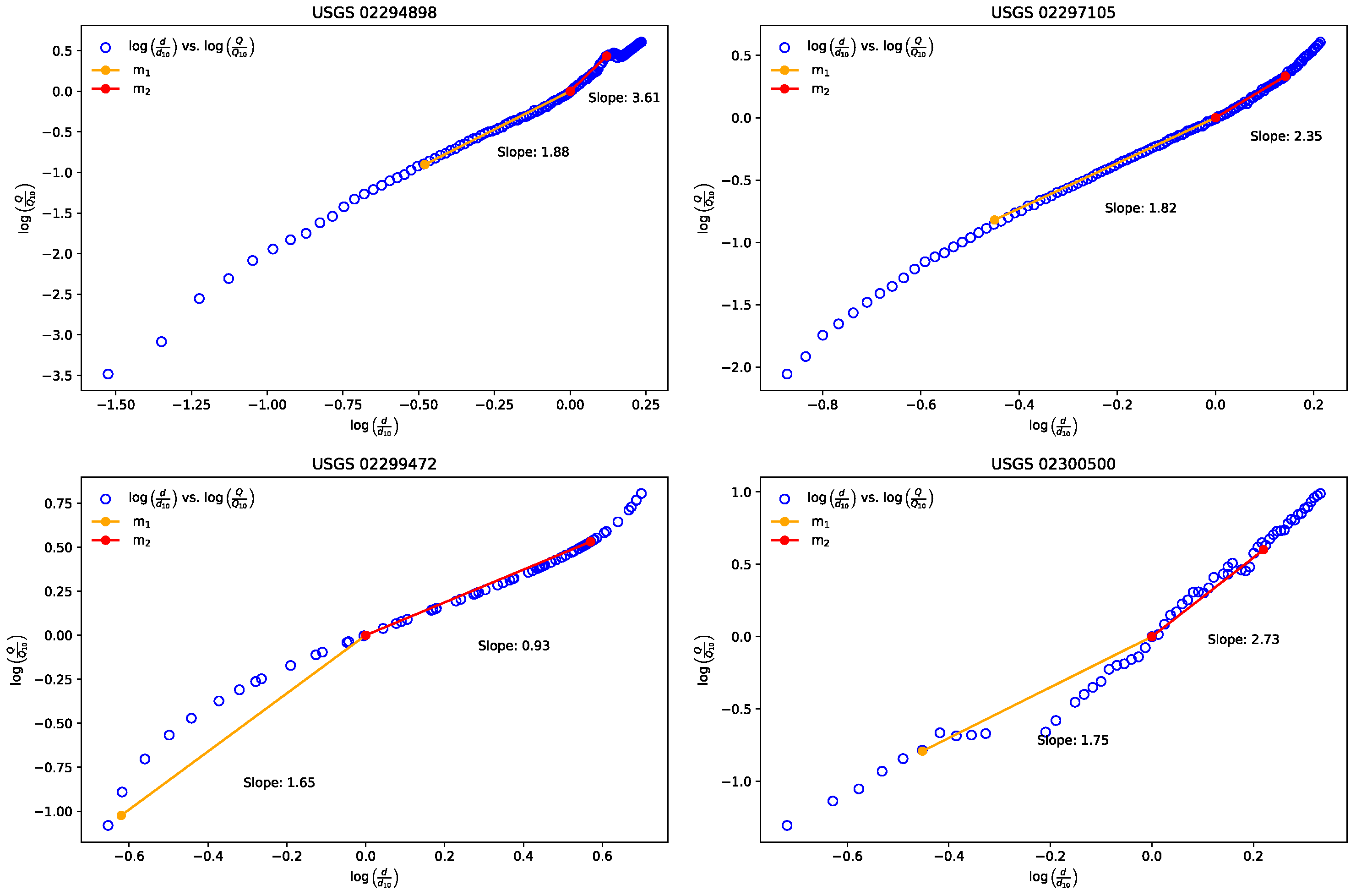
As pointed out previously, the only way to build a depth–discharge relationship in natural streams is by plotting computed depths vs. observed discharges [14]. Plotting the depths against discharges on arithmetic paper over a single control phase or section yields a parabolic line, while plotting them via log–log paper or relations produces a straight line with a constant slope [14]. Plotting a long period of depths and discharges in log–log relations yields straight lines with similar slopes but different offsets that enable hydrologists to dictate the change in control sections, and especially the transition from in-channel control to floodplain control, which is, by definition, beyond bankfull discharge.

The bankfull discharge of an incised channel is the dominant discharge controlling the evolution of the channel geomorphology. Bankfull flow is defined as the channel discharge rate just before the streamflow starts to overflow into floodplain wetlands [18]. Periodic bankfull discharge dictates the channel’s shape, size and invert and thus the depth model [14]. In field measurements, the bankfull depth can often be recognized from stain lines or scour marks and thus measured from the channel bed, vegetation boundaries, transitions between the bed and bank materials, and/or sudden fluctuations on side slopes between channels and floodplains [14]. As a result, the bankfull depth measurement is frequently subjectively interpreted or opinion-based and thus prone to error [14].

The studies on bankfull discharge estimation using reoccurrence interval, which is the exceedance probability of a bankfull discharge in a given year, are inconsistent. Lawlor [22] found that the bankfull discharge reoccurrence interval is between 1 year and 4.4 years, with a median of a 1.5-year recurrence threshold overall. Further supporting this threshold, previous studies showed that the recurrence interval was approximately 1.5-year exceedance [24,25,26,27,28]. However, based on another study by Parrett and Johnson [29], the bankfull discharge at ungauged stations could be calculated through regression of the bankfull discharge to the two-year reoccurrence interval peak discharge. According to Lawlor [22] and previous studies, using a 1.5-year reoccurrence interval to calculate the bankfull discharge for ungauged stations might yield better estimates than the 2-year exceedance threshold. In addition, Mueses et al. [6] sought to develop a non-dimensional discharge rating model by normalizing with respect to bankfull discharge and depth; however, challenges in predicting the bankfull discharge and depth based on the drainage area rendered this approach unviable.

The main goal of this study was to develop a generic model and parameter guideline to produce discharge rating curves for vast ungauged alluvial wetland networks within a continuous hydrologic simulation model. The model seeks to present procedures and parameters for both in-channel and out-of-bank rating. This approach reduces the need for extensive field surveys. It requires only sufficiently resolved Digital Elevation Model(s) (DEMs); commonly available, delineated basins; and cumulative drainage areas. This method enables modelers to establish depth–discharge relationships for any area without direct gauge data, offering a cost-effective and adaptable solution for expansive terrains.

2. Methodology

2.1. Data and Geographic Scope

USGS maintains streamflow gauging stations for numerous streams in southwest Florida. These stations are often monitored through cooperation between USGS and the local water management authorities, such as the Southwest Florida Water Management District (SWFWMD) (Figure 1). USGS measures daily stages for each gauge location relative to a particular datum, either locally established, such as NGVD 1929 or NAVD 88. Also, USGS staff visit gauge sites periodically to report field measurements such as the stage, cross-section area, vegetation condition, width, section control, and discharge. Discharge, stage, and field measurements were downloaded for 90 locations in southwest Florida, including 6 major rivers in the study area: Peace, Manatee, Myakka, Alafia, Withlacoochee, and Hillsborough. These data span from January 1980 to December 2022, covering a full range of flow conditions, including low, medium, and high flows. Some of these stations had no published stages or field measurements and/or were located in areas without DEM data. Data were used based on the availability of information from these stations. Therefore, some of these stations could not be used for all parts of this analysis or to reliably estimate depths or cross-section areas (please refer to

Table 1. Number of USGS stations and corresponding statistics for each variable (with units beside each variable).

Variables	Number of USGS Stations	Maximum	Minimum	Mean	Standard Deviation
Q1 (m3/s)	90	186.61	1.33	28.14	32.49
Q10 (m3/s)	90	75.61	0.22	9.50	13.56
Q50 (m3/s)	90	18.49	0.01	1.54	2.87
A10 (m2)	70	162.58	1.04	30.79	37.96
d1 (m)	83	4.68	0.25	2.21	1.05
d10 (m)	83	3.53	0.14	1.45	0.77
d50 (m)	83	2.65	0.05	0.72	0.5
AD (km2)	90	4726.75	4.14	569.94	958.19
SC (m/m)	70	3.8 × 10−³	5.3 × 10−6	5.5 × 10−4	6 × 10−4

Notes: Q₁₀, Q₅₀, and Q₁ are 10th-, 50th-, and 1st-percentile exceedance discharges, respectively. A₁₀ is the cross-section area at Q₁₀, and d₁₀, d₅₀, and d₁ are 10th-, 50th-, and 1st-percentile exceedance depths, respectively. A_D is the drainage area, and S_C is the channel slope.

for more details).

2.2. Transforming Water Stage Measurements into Depth Values

For reference, USGS does not report the depth of a stream or flow station but monitors the stage and maintains a relationship between the measured stage and discharge. These stage–discharge records and field measurements were used to convert stage–discharge relationships to the depth–discharge relationships required for this analysis. Effective depth (d_e) of flow is relative to a derived depth that is representative of zero flow (even if not measured), which is termed the stream invert or zero flow depth. In the case of perennial stream flow, where no zero flow has been measured, effective depth must be derived from logarithmic extrapolation [6]. The depth used in this analysis is the sum of the invert depth and the difference between the invert stage and the recorded stage. This methodology (referred to as effective depth) was previously presented in Mueses et al. [6]. By calculating the difference between the estimated minimum flow stage (S₀) and the recorded stage (S) and adding the hydraulic mean depth for minimum discharge from the field measurement (d_min) (see also Figure 2), effective depth is

$$d_e=S-S_0+d_{min}$$

(1)

where de is effective depth (L), d_min is minimum hydraulic mean depth (L), S is stage (L), and S₀ is stage at minimum flow (L). It is important to note that the stage for d_min and S₀ often changes with time. Recognizing this change, epics must be identified in the longer-term records to adjust the stage record with time [1,30].

2.3. Improved Non-Dimensional Discharge Rating Curve

Mueses et al. [6] developed a nondimensional model to characterize the depth–discharge rating curve from the reference stage and discharge. Mueses et al. [6] normalized the discharge and depth using the 10th-percentile exceedance discharge, Q₁₀, and the corresponding 10th-percentile depth, d₁₀. Note that these exceedances are daily flows and stages and not annual exceedances. Thus, the 10th-percentile exceedance should be exceeded, on average, 36 days/year. The simple model input included Q₁₀, d₁₀, and m_Mueses which describe the relationship between discharges and depths related to the cross-sectional shape and frictional condition of the channel. Therefore, to develop a discharge rating for an ungauged simulation unit (waterbody), values of Q₁₀, corresponding d₁₀, and m_Mueses must be derived by empirical fitting techniques. The Mueses et al. [6] model is simply

$$\frac{Q}{Q_{10}}={\left[\frac{d}{d_{10}}\right]}^{m_{Mueses}}$$

(2)

where Q₁₀ is the 10th-percentile daily discharge exceedance (L³/T), d₁₀ is the 10th-percentile daily depth exceedance (L), and m_Mueses is Mueses et al.’s [6] discharge behavior exponent. This method has been used with reasonable success to populate and calibrate large regional models in West–Central Florida [31].

M_Mueses was calculated by finding the slope of a best-fit line through the logarithm of normalized depth and discharge values on an arithmetic plot. Thus, the method found the best fit log-linear equation, which is a power law expression of the form

$$\mathit{log}\left(\frac{Q}{Q_{10}}\right)=m_{Mueses}·\mathit{log}(\frac{d}{d_{10}})+\mathit{log}(b)$$

(3)

where b is the intercept.

Using a construction method that involved the hydraulic depth of the lowest flow measurement to establish the depth at zero flow, even if it did not exist in the observations, the intercept (b) was eliminated.

A modified version of the Mueses et al. [6] non-dimensional model was formulated to better reproduce discharge rating curves in this study using GIS deliverable variables. The hypothesis behind the modified approach is that when the streamflow depth is within the channel bank (in-bank flows), the discharge rating curve follows one exponent. That exponent changes after the transition to out-of-bank discharges (floodplain stages). Smoothness in the discharge rating is ensured by using a common reference index. Breaks in discharge rating curves for flood flows (out-of-bank flows) have been well documented [14]. The modified method applies two exponents. The first exponent reproduces the discharge rating curve for discharges less than Q₁₀, and the second reproduces the discharge rating curve for discharges higher than Q₁₀. To help adapt the method to be used for ungauged hydro-features, the model low- and medium-flow (in-bank) exponent (m₁) was calculated from the 50th-percentile exceedance flow and depth, Q₅₀ and d₅₀, respectively, and the exponent for out-of-bank flows (m₂) was calculated from the 1st-percentile exceedance flow and depth, Q₁ and d₁.

The relationships found for the exponents are

$$m_1=\frac{\mathit{log}\left(\frac{Q_{50}}{Q_{10}}\right)}{\mathit{log}\left(\frac{d_{50}}{d_{10}}\right)}$$

(4)

$$d=d_{10}{\left[\frac{Q}{Q_{10}}\right]}^{\frac{1}{m_1}}$$

(5)

For m₂, the out-of-bank exponent is

$$m_2=\frac{\mathit{log}(\frac{Q_1}{Q_{10}})}{\mathit{log}(\frac{d_1}{d_{10}})}$$

(6)

$$d=d_{10}{\left[\frac{Q}{Q_{10}}\right]}^{\frac{1}{m_2}}$$

(7)

where Q₁₀ and d₁₀ were previously defined; Q₅₀ is the 50th-percentile daily exceedance discharge (L³/T); Q₁ is the 1st-percentile exceedance discharge (L³/T); d₅₀ and d₁ are the 50th- and 1st-percentiles exceedance effective depths (L), respectively; m₁ is the exponent for in-bank discharges; and m₂ is the exponent for out-of-bank discharges.

When the rating curves of USGS flow stations were studied, a trend was observed in these rating curves. Figure 3 shows four normalized rating curves of the studied gauge stations, each characterized by varying drainage areas ranging from 222 to 4325 km². This figure is pivotal in highlighting the behaviors of m₁ and m₂, demonstrating variations in the slope of the rating curve before and after the Q₁₀ (0,0) point.

Observations revealed that Q₁₀, typically not associated with out-of-bank discharge, remained within bank limits for these streams. A closer examination of the rating curve showed that Q₁₀ is a critical transition point for the onset of out-of-bank behavior. Mathematically, Q₁₀ serves as an ideal marker for identifying the beginning of out-of-bank flow, primarily due to its position at the lower end of this transition phase.

This study also utilized Q₅₀ to represent both mean and minimum flows. As Q₅₀ is the median flow, it was deemed a reliable indicator. However, the accuracy of low-flow measurements was often compromised by factors like deposition, erosion, or channel obstructions, which could alter the rating curve and affect measurement precision. It was suggested that Q₅₀ is the most reliably predictable low-flow percentile discharge.

Furthermore, Q₁ was selected to characterize out-of-bank behavior. The methodology focused on using a flow metric that could both accurately predict and represent high-flow conditions. Attempts to model extremely high flows, specifically the 0.01st-percentile exceedance flow (Q_0.01), resulted in an R² of 0.5. Consequently, Q₁ was chosen as the representative metric for high flows. Therefore, Q₁₀ was used to delineate the shift from in-bank behavior (m₁) to out-of-bank behavior (m₂), as further detailed in Figure 3.

2.4. Estimations of Q₁₀, Q₅₀, and Q₁

The drainage area size, A_D, and physical watershed characteristics are the key variables for regulating hydrologic fluxes within an environment with similar climatic and topographic conditions [17,23]. While the A_D is by far the most significant, other physical characteristics such as the watershed slope, wetland and upland vegetative cover, urban landform percentage (and imperviousness), soil type, and proximity of the water table to land surface play a lesser role in determining the high-flow (index) discharge rate within a single environment, especially for larger areas [1,30,32]. This is because the variability of these influences for larger watersheds in many environments, including the study area in southwest Florida, is small. Mueses et al. [6] and Mueses [30] examined variables derivable from GIS coverages influencing Q₁₀. The conclusion was A_D is the only parameter showing a strong correlation.

The purpose of this simplified analysis was to identify relationships that can estimate these reference discharges for ungauged hydro-features (where no discharge rating data exist) and in vast hydrography settings, typical of larger regional models. It is important to point out that these exceedances follow a non-normal distribution and are skewed in generally predictable ways [33]. For these data, the accuracy of parametric tests, which measure the fit of linear regression models, is invariably poor [33]. The normality of these reference discharges was tested graphically using a Q-Q plot [33], and the results show the expected non-normality distribution (Figure 4). Therefore, the discharge datasets were logarithmically transformed (log Q values) to make the distribution symmetrical and normal (Figure 5). Then, the Q₁, Q₅₀, and Q₁₀ for 90 gauge stations were randomly divided into training and test datasets, with a heavier weight toward the training dataset (80% of the data), while the test dataset contained the remaining 20%. The training dataset was linearly regressed, and the resultant estimators were tested using parametric tests against the test dataset to evaluate the fit quality. The results were then evaluated using R², which is the variation of the discharges that the drainage area can explain.

2.5. Estimation of A₁₀

As pointed out previously, USGS visits streamflow gauges for low, medium, and high discharges multiple times annually and takes field measurements such as velocity, stage, and cross-section area. These data are generally published online as field notes for the gauging stations. The time series of cross-section areas from 70 streamflow gauge stations with suitable high-resolution DEM data in southwest Florida were used to derive a relationship for estimating the cross-section area at Q₁₀, A₁₀, for each station.

SWFWMD produced high-resolution 1.5 m horizontal, vertical accuracy < 0.1 m (5 ft horizontal, vertical accuracy < 0.3 ft) DEM for southwest Florida regions to estimate the local longitudinal channel slopes, S_c, and channel width, W_C. The S_c of 70 gauge stations was estimated by determining the elevation at the gauge station and approximately a thousand meters upstream of the gauge station. W_C was also calculated by measuring the width of the channel from the DEM using a GIS measure tool at the gauge locations.

The A_D and the S_c^0.5 for these streamflow gauging stations were logarithmically transformed because of non-normality (Figure 4 and Figure 5) and divided into training and test datasets, with 80% allocated to the training set and 20% to the test set. Then, the training data were used in a multiple-variables linear regression model to estimate the A₁₀. Then, the model was tested against the test dataset, again by regression. The multiple-variables linear regression model was evaluated using R².

2.6. Estimations of d₁₀, d₅₀, and d₁

Three linear regression models were developed: one to predict d₁₀ using the hydraulic mean depth at Q₁₀, d_h10, and the other two models to predict d₁ and d₅₀ using d₁₀. d_h10 for 83 streamflow gauge stations was calculated from observed discharge rating curves by dividing A₁₀ (L²) by W_C (L) and then regressed to estimate d₁₀ (L). d₁₀ was estimated using the Mueses et al. [6] method for effective depth. The stage at Q₁₀ was subtracted from the minimum flow stage and added to the hydraulic mean depth of the lowest field measurement. A similar method was employed to estimate d₁ and d₅₀. Then, the data were divided into training and test datasets of 80% and 20%, respectively. Finally, d₁₀ for 66 of the 83 streamflow gauge stations was regressed to estimate d₁ and d₅₀. Then, the results were evaluated against the test dataset. The regression model accuracy of predicting d1 and d₅₀ was evaluated using R².

$$d_{h10}=\frac{A_{10}}{W_C}$$

(8)

where d_h10 is the hydraulic-mean depth of Q₁₀ (L), A₁₀ is the cross-section area of Q₁₀ (L²), and W_C is the width of Q₁₀ (L).

2.7. m_Mueses vs. m₁ (in Channel Flow Exponent)

As discussed earlier, a single Mueses’ exponent performed poorly for discharges higher than Q₁₀. Therefore, at a minimum, there is a need to use two exponents to describe the full range of discharge ratings, including discharges below and above Q₁₀ (in- and out-of-bank flows). The required work to generate a m_Mueses value is only possible with extensive flow measurement data. Hence, as the method is desired to populate the vast ungauged hydrography in a regional model domain, the m₁, derived from Equation (4) using observed Q₁₀, Q₅₀, d₁₀, and d₅₀, was compared against m_Mueses. Then, m_Mueses and m₁ were evaluated using R². On the other hand, the exponent for discharges higher than Q₁₀, m₂, was produced using Equation (6) but was not used in the comparison since m₂ was introduced within this study.

2.8. Testing and Verification: Addressing Uncertainty

Regression models were formulated to estimate discharge rating parameters using three readily derivable variables for any ungauged simulation unit: A_D, S_c, and W_C. These determinants were applied within the regression models to generate predictions for Q₁₀, Q₅₀, Q₁, d₁₀, d₅₀, and d₁. Following this, m₁ and m₂ were derived from Equations (4) and (6). The precision of these forecasts was gauged via the Root Mean Squared Error (RMSE) and Mean Error (ME). Subsequently, these predictions were employed in Equations (5) and (7) to reproduce the USGS discharge rating curves. Then, the replicated discharge rating curves were compared to the observed USGS discharge rating curves. Also, the original model from Mueses et al. [6] for ungauged simulation units was compared to the observed USGS discharge rating curves. Then, the accuracy was evaluated through RMSE and ME.

3. Results

3.1. Predicting Q₁₀, Q₅₀, and Q₁

Predicting the exceedance discharges for Q₅₀, Q₁₀, and Q₁ using only A_D showcased strong performance. Specifically, R² values for the training dataset were 0.78, 0.9, and 0.84 for Q₅₀, Q₁₀, and Q₁, respectively. For the test dataset, the R² values for Q₅₀, Q₁₀, and Q₁ were statistically comparable, with values of 0.76, 0.89, and 0.81, respectively (see Figure 6). The derived linear equations are as follows:

$$Log\left(Q_{50}\right)=0.9Log\left(A_D\right)-2.38$$

(9)

$$Log\left(Q_{10}\right)=0.81 Log\left(A_D\right)-1.2$$

(10)

$$Log\left(Q_1\right)=0.67 Log\left(A_D\right)-0.32$$

(11)

where Q₅₀, Q₁₀, and Q₁ were previously defined (m³/s), and A_D is the drainage area in (km²).

3.2. Predicting A₁₀

The multi-variable linear regression model using A_D and S_c^0.5 demonstrated a robust relationship for the A₁₀. For the training and test datasets, the R² values were 0.87 and 0.92, respectively. Notably, the p-values for A_D and S_c^0.5 were less than 0.0000. A₁₀ exhibited a positive relationship with A_D and a negative relationship with S_c^0.5 (see Figure 7). The results indicated that, statistically, A_D and S_c^0.5 are reliable estimators for A₁₀, as

$$Log\left(A_{10}\right)=0.69Log\left(A_D\right)-0.72Log\left({S_c}^{0.5}\right)-1.62$$

(12)

where A₁₀ (m²) and A_D (km²) were previously defined, and S_c^0.5 is the channel slope (m/m).

3.3. Predicting d₁₀, d₅₀, and d₁

The model’s ability to predict the different percentile exceedance depths was evaluated. The R² for the training datasets of d₁₀, d₅₀, and d₁ were 0.85, 0.77, and 0.88, respectively, and R² for the test datasets for these same variables was substantially equivalent at 0.87, 0.78, and 0.9, respectively (see Figure 8). The results conclusively showed that d_h10 can be used to estimate d₁₀, d₅₀, and d₁, and the resulting equations (for units of meter) are

$$Log\left(d_{10}\right)=0.84\mathit{Log}\left(d_{h10}\right)+0.16$$

(13)

$$Log\left(d_{50}\right)=0.99\mathit{Log}\left(d_{10}\right)-0.34$$

(14)

$$Log\left(d_1\right)=0.86\mathit{Log}\left(d_{10}\right)+0.21$$

(15)

where d_h10, d₁₀, d₅₀, and d₁ were previously defined (m).

3.4. m_Mueses vs. m₁ (in Channel Flow Exponent)

The exponent, m_Mueses, proposed by Mueses et al. [6], represents the best-fitted line through normalized depths and discharges of the discharge rating curves. When linearly regressed against the in-bank exponent of the refined model, m₁, calculated from Q₁₀, Q₅₀, d₁₀, and d₅₀, it yielded an R² value and slope close to 1 (≈45°), as depicted in Figure 9.

3.5. Assessing Uncertainty in Parameter Estimation and Rating Curve Reproduction

When the A_D of 70 gauge stations was used in the proposed linear regression models to predict Q₁₀, Q₅₀, and Q₁, the RMSE values were 4.98 m³/s, 1.04 m³/s, and 13.37 m³/s, respectively. While the ME exhibited small bias in all predicted discharges, the ME values were −1.38 m³/s, −0.35 m³/s, and −4.21 m³/s, respectively. Also, when A_D, S_c^0.5, and W_C were used to predict A₁₀, d₁₀, d₅₀, and d₁, the RMSE values were 18.81 m², 0.64 m, 0.34 m, and 0.88 m, respectively. While the ME exhibited a small bias as well, the values were −2.75 m², −0.02 m, −0.01 m, and −0.04 m, respectively. The observed bias in the results was expected, given the diverse streamflow gauge stations utilized to predict each parameter within the linear regression models. These predictions were subsequently tested across 70 streamflow gauge stations, some of which were part of the training dataset while others were not (please refer to

Table 2. The Root Mean Squared Error (RMSE) and Mean Error (ME) of the developed regression models (with units beside each variable).

Variables	RMSE	ME
Q10 (m3/s)	4.98	−1.38
Q50 (m3/s)	1.04	−0.35
Q1 (m3/s)	13.37	−4.21
A10 (m2)	18.81	−2.75
d10 (m)	0.64	−0.02
d50 (m)	0.34	−0.01
d1 (m)	0.88	−0.04

Notes: Q₁₀, Q₅₀, Q₁, A₁₀, d₁₀, d₅₀, and d₁ were previously defined.

for more details).

Compared with the Mueses et al.’s [6] model, the improved model performance was superior across different RMSE ranges. For an RMSE of $\le$0.3 m (≈≤1 ft), the improved model showed that 40% of the stations (28 out of 70) achieved this accuracy, compared to 25.7% (18 out of 70 stations) in the Mueses et al. [6] model. In the RMSE range of 0.3 to 0.6 m (≈1 to 2 ft), 50% of stations fell under the improved model, whereas only 32.86% did so under the Mueses model. In the improved model, 90% of the stations achieved an RMSE ≤ 0.6 m (≤2 ft), compared to only 58% of stations achieving this range with the Mueses model. A more detailed performance analysis for higher RMSE ranges, along with the corresponding percentages of stations, is outlined in Table 2 and illustrated in Figure 10. The average RMSE was notably lower in the improved model at 0.38 m (≈1.24 ft), compared to 0.67 m (≈2.2 ft) in the Mueses model, reflecting a significant enhancement in prediction accuracy. For a detailed comparison of these models across different RMSE ranges, refer to

Table 3. The comparative analysis of RMSE in streamflow predictions at 70 USGS gauge stations: improved model vs. Mueses et al. [6] model.

RMSE (m)	USGS Percentage of Stations within RMSE Range (%)
	Improved Model	Mueses Model
0 to 0.3 (≈0 to 1 ft)	40%	25.71%
0.3 to 0.6 (≈1 to 2 ft)	50%	32.86%
0.6 to 0.9 (≈2 to 3 ft)	7.14%	24.29%
0.9 to 1.2 (≈3 to 4 ft)	1.43%	5.71%
1.2 to 1.5 (≈4 to 5 ft)	1.43%	2.86%
1.5 to 1.8 (≈5 to 6 ft)	0%	1.43%
1.8 to 2.1 (≈6 to 7 ft)	0%	1.43%

and Figure 10.

The discharge rating curves generated by the improved model (d′), Mueses et al. [6] model (d_Mueses), and the observed data from USGS streamflow gauge stations (d) were plotted for three different locations, each characterized by a unique A_D. The improved model demonstrated robust performance in simulating observed discharge rating curves for low and high-flow conditions at all three locations. This enhanced accuracy can be attributed to applying dual exponents and integrating both Sc and Wc within the model framework. On the other hand, the Mueses model, which predominantly relies on drainage area as the predictor, was found to underestimate the observed discharges at A_D of 530 km² (Figure 11c) generally. At a larger drainage area of 3540 km², the model tended to overestimate the observed behavior, underscoring the limitations inherent in using only A_D as the independent variable for developing discharge rating curves. For further details, refer to Figure 11.

4. Discussion, Recommendations, and Limitations

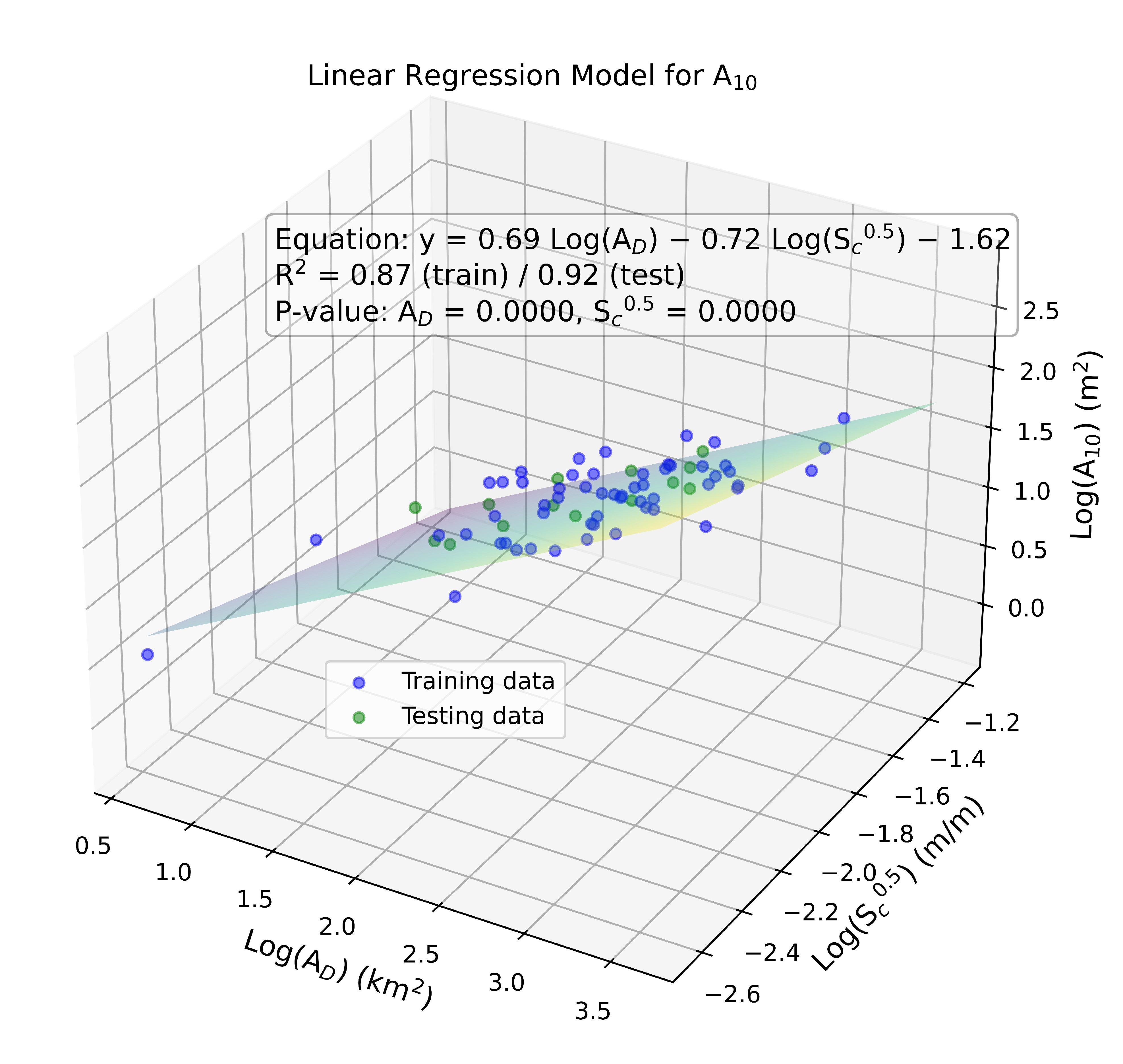
This study’s objective was to develop a more reliable method to characterize the depth–discharge relationship for ungauged alluvial stream/wetland systems. Using commonly available GIS data and simple relationships, the method has been tested for southwest Florida hydrology and demonstrated improved performance compared to the earlier procedures presented by Mueses et al. [6]. The method uses minimal calibration parameters and can be used or adapted for other environments. Since the drainage area size is the most important variable and previous studies indicated much lower sensitivity to other variables such as upland land use and watershed slope, it is believed that this variable, together with a GIS determination of longitudinal channel slope and transverse width, can be used to estimate the important controlling factors of A₁₀, d₁₀, Q₁₀, and in-bank and out-of-bank discharge rating exponents, m₁ and m₂, for applications where measured cross-sections and discharge rating conditions are sparse.

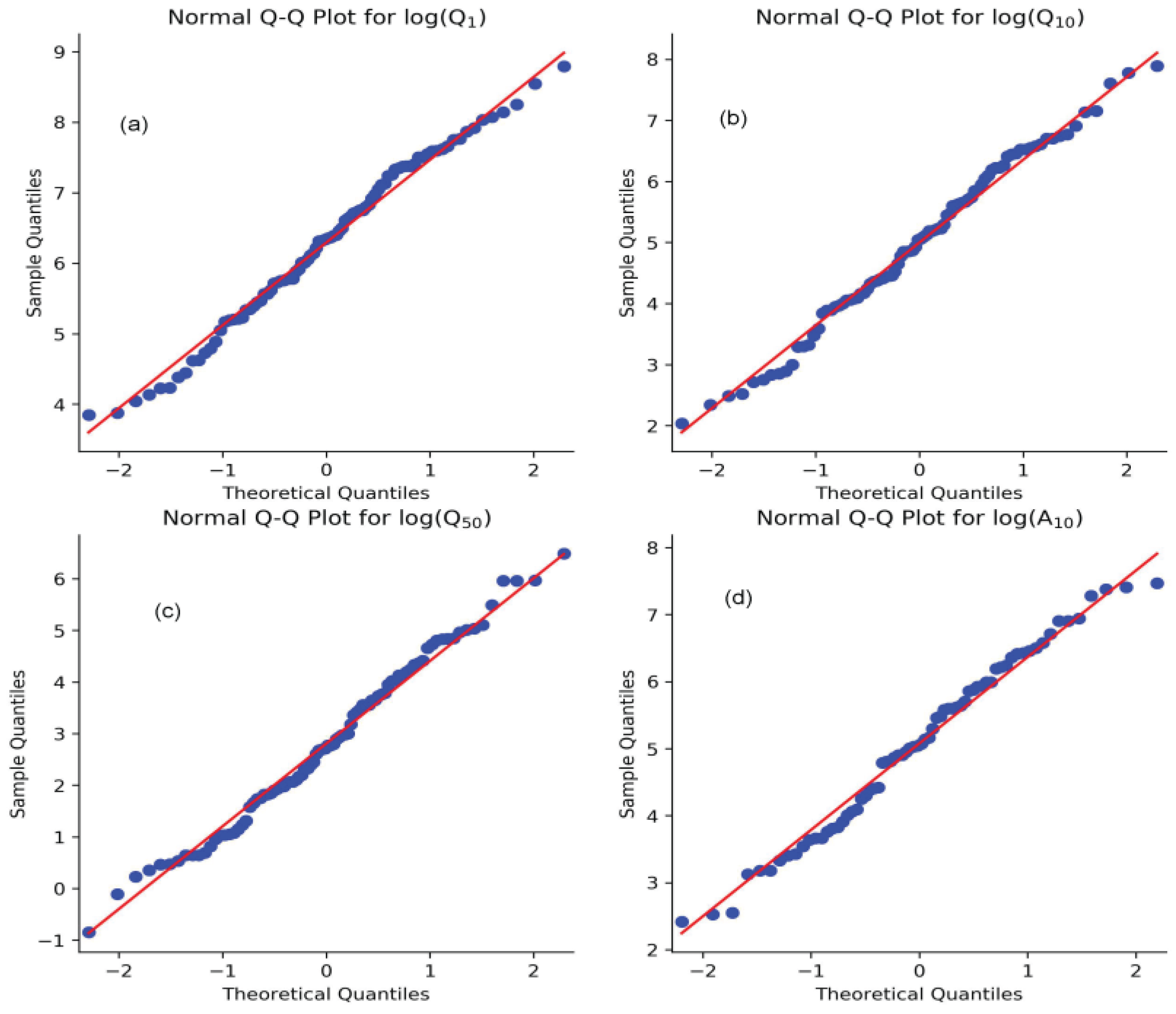
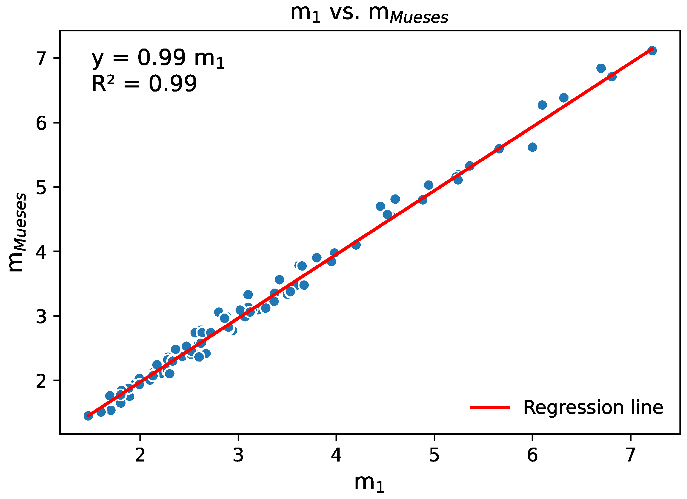
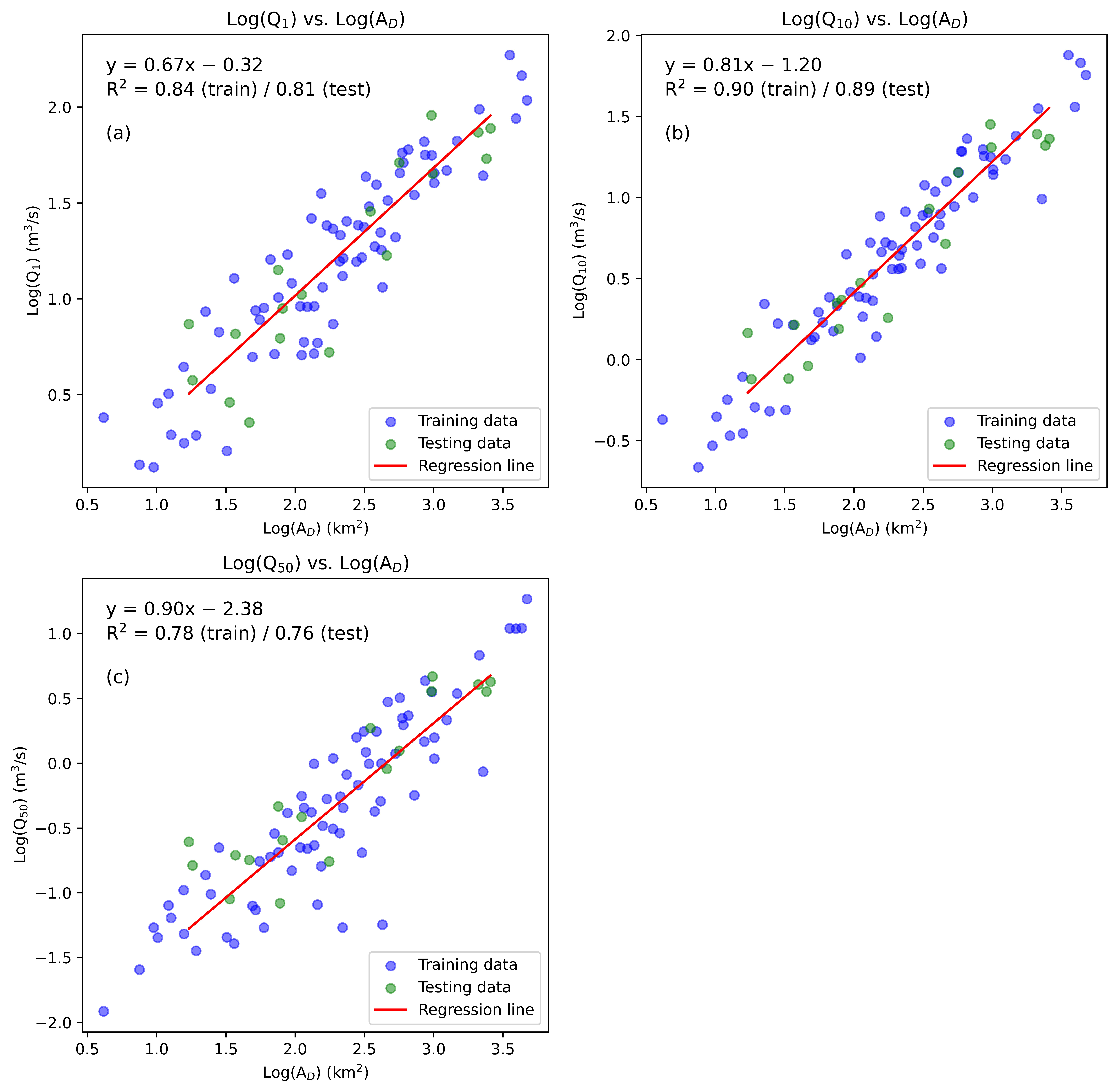
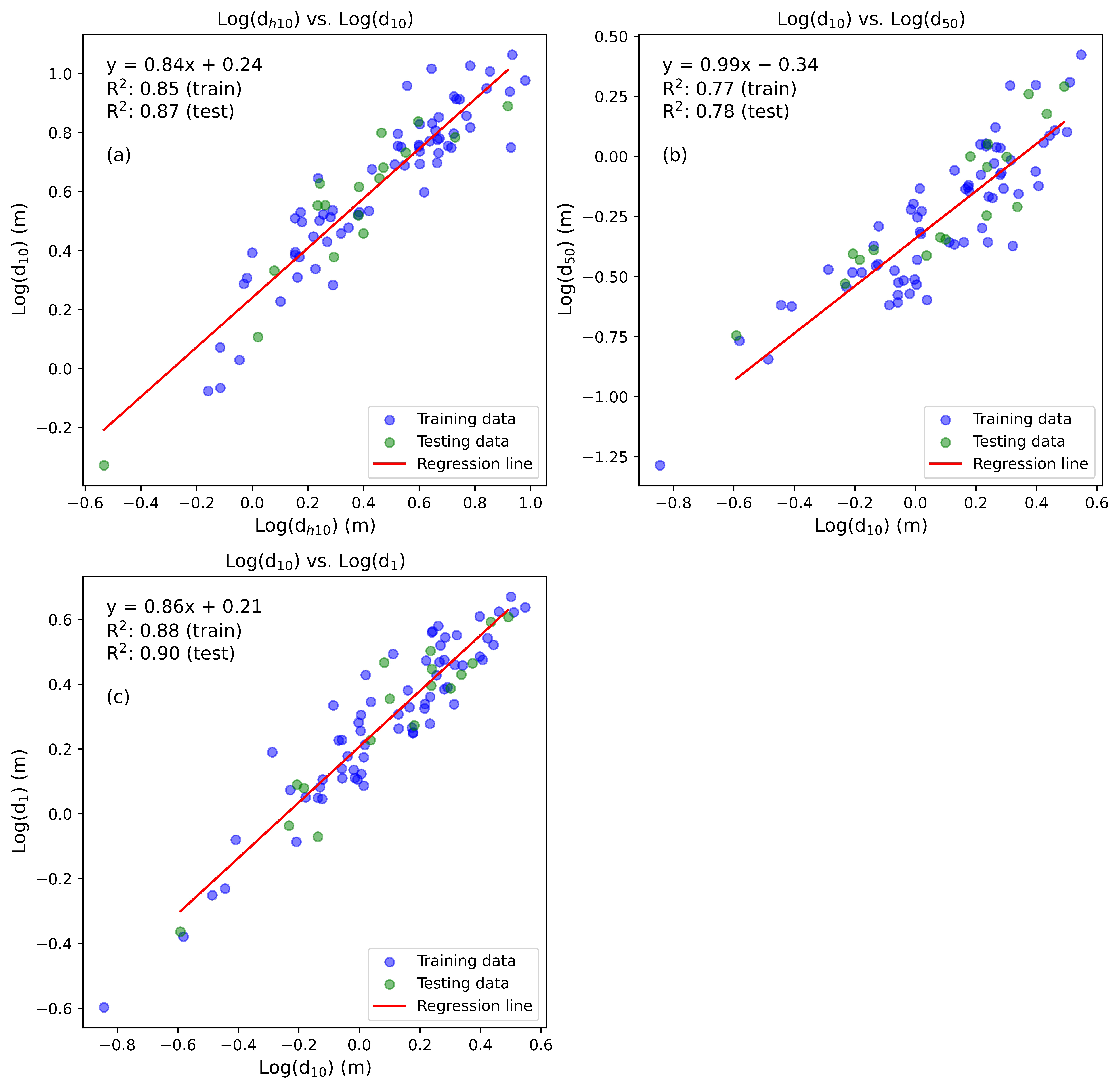
Providing separate exponents for in-bank and out-of-bank discharge ratings greatly increases the accuracy and physical basis of the approach. However, for ungauged sections, doubling the number of uncertain parameters would lead to overparameterization if an objective means to define both were unavailable. This approach indicated that adding another flow index, Q₅₀, could be used to help predict the in-bank flow exponent, m₁. Since Q₅₀ was found to be strongly correlated to drainage area and, by definition, represents the median flow behavior, it was shown to suitably provide for the determination of the low-flow (in-bank) discharges and the appropriate exponent, m₁.

For higher flows, Q₁ was also shown to be strongly correlated to the drainage area, and this flow represents a likely out-of-bank or near-bankfull flow condition. This flow index has a lower probability of occurrence and is observed for approximately only 3 days per year on average. Since it is appropriate for high flows and for convenience, it was selected to provide a method to estimate the high-flow behavior, m₂, and showed acceptable predictive performance. However, where data exist for out-bank behavior, discharge exceedances with extremely low probability, such as the 0.01 percentile conditions, can be utilized. It should be noted that these percentile exceedances refer to daily, rather than yearly, occurrences.

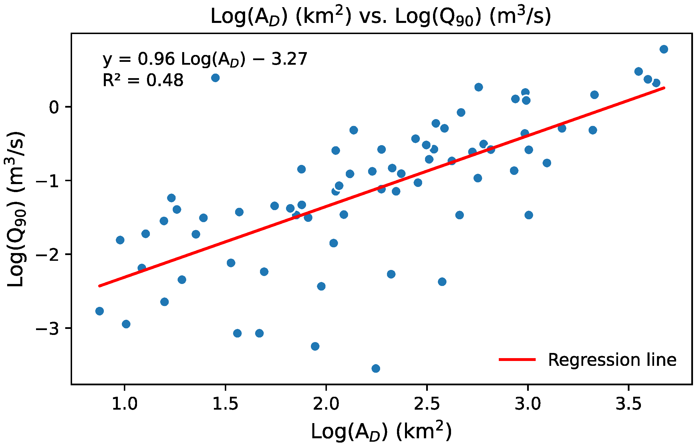
Not surprisingly, the 90-percentile exceedance discharge was not suitably dependent on the drainage area (Figure 12), perhaps due to the strong sensitivity to baseflow and groundwater processes, and thus provided an index that was not useful for this method. Furthermore, natural streams experience live bed processes, shifting bed materials, and sensitivity to fallen debris, making the discharge rating curve behavior for low flows unreliable or even unstable. As a result, Q₅₀ is believed to be the lowest index that is suitable for describing the medium- and low-flow discharge rating behavior.

The southwest Florida region is mostly characterized as a low-slope environment (generally <0.3%) with protected alluvial floodplain wetlands, where natural streams tend toward uniform flow more often than higher-gradient systems. This may be one reason the concept of a fixed and predictable discharge rating behavior prevails and seems appropriate.

Relating the drainage area to depth assumes that when the drainage area is increasing, the depth is also, which is not always the case considering channel width variability. However, switching to a cross-sectional area dependence (A₁₀), assuming that the cross-sectional area is directly related to the magnitude of Q₁₀, is conceptually sound and has been shown to be a better basis for defining d₁₀. Hence, GIS procedures or other interpretations will be needed to define the hydraulic (or top-of-bank) width for Q₁₀.

The primary limitation of this study is that the empirical relationships may differ in other environmental settings, particularly in highly variable alluvial systems (e.g., anthropogenetic and hardened channel settings). This is because it can be challenging to ascertain whether channels in such settings are fully developed and contain any relation to flow return probability (index). The difficulty lies in determining if these channels have evolved between regular flow states and the erosion susceptibility of channel morphology. In sandy-terrain Florida, channels are highly variable in degree of incision, some deeply incised, others not, but are in relative dynamic equilibrium with probabilistic flows and cross-section relation, leading to a strong relationship between drainage area and cross-sectional area. This would likely not be the case in artificially hardened or natural rock-bed channels in non-depositional environments. However, even with different soil types, land use, and hydrology in coastal plain environments, these empirical relationships will likely still be applicable, but some local adjustments to the coefficients may be necessary. To apply this methodology in a new environment, it will be essential to have a sufficient number of gauge stations with extensive records of in-bank and out-of-bank discharges to validate the approach and coefficient behavior. Additionally, observational verification of the method in different settings may prove to indicate yet another variable or process that becomes important. In the absence of a sufficiently resolved DEM, channel width and slope must be manually determined from topographic data or estimated by the user.

5. Conclusions

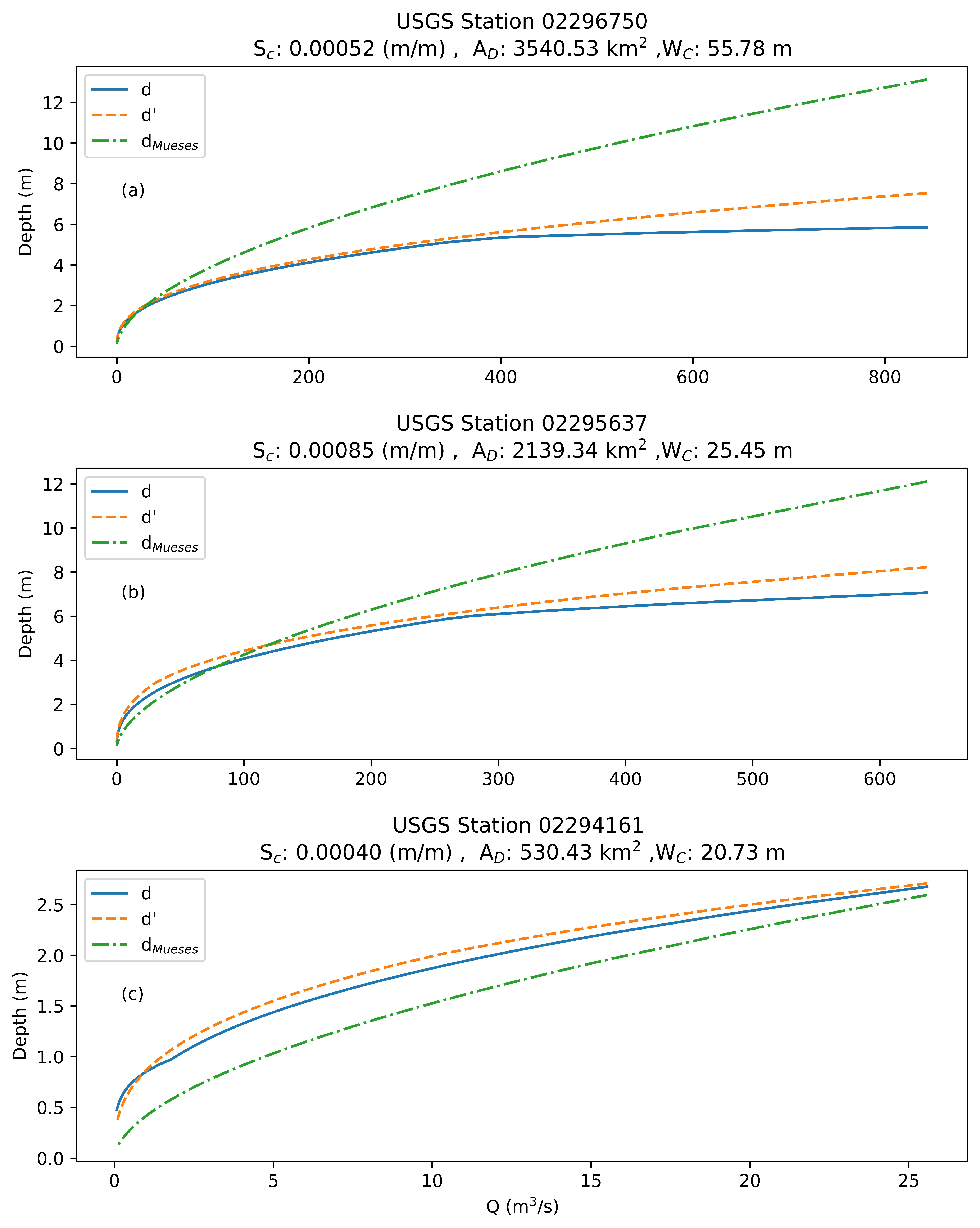
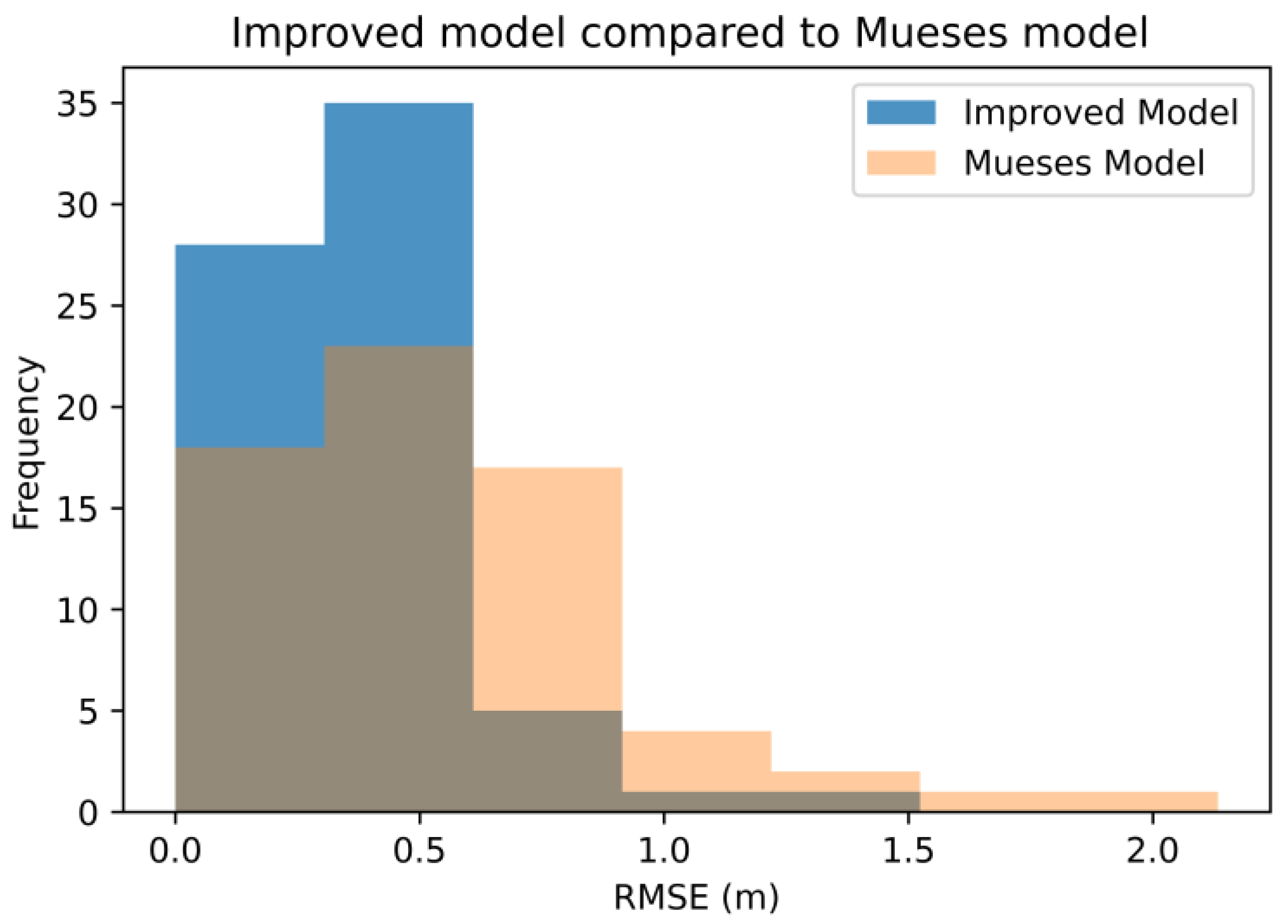
This study sought to develop a more reliable method for characterizing the depth–discharge relationship in dendritic alluvial stream/wetland systems for hydrologic modeling where limited or sparse gauge or survey data are available. The method uses simple GIS and normalized analyses based on derivable flow indexes defined for each channel section. The improved procedure simply requires cumulative drainage area, local channel slope, channel width, and readily derivable GIS data to develop discharge ratings for gauged and ungauged sections. The discharge rating curves for 70 USGS streamflow gauges were reproduced using the procedure, and then the produced and observed discharge rating curves were compared to evaluate the accuracy of the method. The methodology developed demonstrated improved performance compared to previous methods with minimal calibration parameters.

The comparison showed robust performance in predicting depth with minimal errors. In the analysis of streamflow depth predictions, the average RMSE was 0.38 m (≈1.24 ft), with an interquartile range between 0.21 m and 0.49 m. The ME showed no bias (centered around 0 m), with manageable interquartile values ranging +/−0.24 m.

The approach relied heavily on the cumulative drainage area to each reach (A_D), which was found to be the most significant variable. By combining GIS-determined channel slopes (S_c) and width (W_C), as well as key flow and depth indexes of d₁₀, d₅₀, and d₁, and Q₁₀, Q₅₀, and Q₁, discharge rating exponents m₁ and m₂ can be estimated, which were shown to be reliable for predicting in-bank and flood flow (out-of-bank) discharge ratings. This study found strong relationships between Q₅₀ and A_D for low-flow discharges and between Q₁ and A_D for high flows, aiding in estimating the respective exponents m₁ and m₂.

The success of the approach in the studied Florida region, characterized by similar vegetation and slopes in fully developed (depositional equilibrium) floodplain wetlands, suggests potential applicability in other coastal plain environments. Adjustments may be necessary in different environmental settings, particularly where channels have high variability or are not in full depositional equilibrium. However, success and confidence in other settings will require sufficient gauging stations and adequate GIS data before validating the approach.

References

1. Sivakumar, B. Global climate change and its impacts on water resources planning and management: Assessment and challenges. Stoch. Environ. Res. Risk Assess. 2011, 25, 583–600. [Google Scholar] [CrossRef]
2. Liu, Y.; Engel, B.A.; Flanagan, D.C.; Gitau, M.W.; McMillan, S.K.; Chaubey, I. A review on effectiveness of best management practices in improving hydrology and water quality: Needs and opportunities. Sci. Total Environ. 2017, 601–602, 580–593. [Google Scholar] [CrossRef] [PubMed]
3. Gupta, R.S. Hydrology and Hydraulic Systems; Waveland Press: Long Grove, IL, USA, 2016. [Google Scholar]
4. Ross, M.A.; Geurink, J.S. Integrated Hydrologic Model Version 3 Theory and Implementation; Tampa Bay Water: Clearwater, FL, USA; Brooksville, FL, USA, 2018. [Google Scholar]
5. Devia, G.K.; Ganasri, B.P.; Dwarakish, G.S. A Review on Hydrological Models. Aquat. Procedia 2015, 4, 1001–1007. [Google Scholar] [CrossRef]
6. Mueses, A.; Said, A.; Ross, M. Generalized Nondimensional Depth-Discharge Rating Curves Tested on Florida Streamflow. J. Am. Water Resour. Assoc. 2007, 43, 473–481. [Google Scholar] [CrossRef]
7. Liu, Z.; Wang, Y.; Xu, Z.; Duan, Q. Conceptual Hydrological Models. In Handbook of Hydrometeorological Ensemble Forecasting; Duan, Q., Pappenberger, F., Thielen, J., Wood, A., Cloke, H.L., Schaake, J.C., Eds.; Springer: Berlin/Heidelberg, Germany, 2017; pp. 1–23. ISBN 978-3-642-40457-3. [Google Scholar]
8. Bicknell, B.R.; Imhoff, J.C.; Kittle, J.L.; Donigian, A.S. Hydrological Simulation Program—Fortran User’s Manual for Release 1; US Environmental Protection Agency: Athens, Greece, 1997.
9. Rossman, L.A. Storm Water Management Model User’s Manual Version 5.1; EPA: Washington, DC, USA, 2015.
10. Normand, A.E. U.S. Geological Survey (USGS) Streamgaging Network: Overview and Issues for Congress; Congressional Research Service: Washington, DC, USA, 2021.
11. Carter, R.W.; Davidian, J. General Procedure for Gaging Streams; U.S. Geological Survey: Reston, VA, USA, 1968; p. 13. [Google Scholar] [CrossRef]
12. Mansanarez, V.; Renard, B.; Coz, J.L.; Lang, M.; Darienzo, M. Shift Happens! Adjusting Stage-Discharge Rating Curves to Morphological Changes at Known Times. Water Resour. Res. 2019, 55, 2876–2899. [Google Scholar] [CrossRef]
13. Rantz, S.E. Measurement and Computation of Streamflow: Volume 2. Computation of Discharge; U.S. Department of the Interior: Washington, DC, USA, 1982; Volume 2, p. 389. [Google Scholar]
14. Gordon, N.D.; McMahon, T.A.; Finlayson, B.L.; Gippel, C.J.; Nathan, R.J. Stream Hydrology: An Introduction for Ecologists; John Wiley and Sons: Hoboken, NJ, USA, 2004. [Google Scholar]
15. Kennedy, E. Discharge Ratings at Gauging Stations. Techniques of Water Resources Investigations of the U.S. Geological Survey, USGS Book 3, Chapter A10; USGS: Alexandria, VA, USA, 1984.
16. Lewelling, B. Extent of Areal Inundation of Riverine Wetlands along Five River Systems in the Upper Hillsborough River Watershed, West-Central Florida. In U.S. Geological Survey Scientific Investigation Report 2004-5133; USGS: Alexandria, VA, USA, 2003; p. 49. [Google Scholar]
17. Emmett, W.W. The Channels and Waters of the Upper Salmon River Area, Idaho; Professional Paper; USGS: Alexandria, VA, USA, 1975.
18. Leopold, L.B.; Wolman, M.G.; Miller, J.P. Fluvial Processes in Geomorphology: San Francisco; W.H. Freeman and Company: New York, NY, USA, 1964; p. 522. [Google Scholar]
19. Braca, G. Stage-Discharge Relationships in Open Channels: Practices and Problems; Università degli Studi di Trento, Dipartimento di Ingegneria Civile e Ambiental: London, UK, 2008. [Google Scholar]
20. Acreman, M.; Holden, J. How Wetlands Affect Floods. Wetlands 2013, 33, 773–786. [Google Scholar] [CrossRef]
21. Ashley, G.M.; Renwick, W.H.; Haag, G.H. Channel form and processes in bedrock and alluvial reaches of the Raritan River, New Jersey. Geology 1988, 16, 436. [Google Scholar] [CrossRef]
22. Lawlor, S. Determination of Channel-Morphology Characteristics, Bankfull Discharge, and Various Design-Peak Discharges in Western Montana; Scientific Investigations Report; USGS: Alexandria, VA, USA, 2004.
23. Dunne, T.; Leopold, L.B. Water in Environmental Planning; W.H. Freeman: San Francisco, CA, USA, 1978; p. 818. [Google Scholar]
24. Castro, J.M.; Jackson, P.L. Bankfull discharge recurrence intervals and regional hydraulic geometry relationships: Patterns in the pacific northwest, USA 1. JAWRA J. Am. Water Resour. Assoc. 2001, 37, 1249–1262. [Google Scholar] [CrossRef]
25. Cinotto, P.J. Development of Regional Curves of Bankfull-Channel Geometry and Discharge for Streams in the Non-Urban, Piedmont Physiographic Province, Pennsylvania and Maryland (No. 3); US Department of the Interior: Washington, DC, USA; US Geological Survey: Reston, VA, USA, 2003.
26. Moody, T.O.; Odem, W. Regional Relationships for Bankfull Stage in Natural Channels of Central and Southern Arizona; Northern Arizona University, College of Engineering and Technology: Flagstaff, AZ, USA, 1999. [Google Scholar]
27. Rosgen, D.L.; Silvey, H.L. Applied River Morphology (Vol. 1481); Wildland Hydrology: Pagosa Springs, CO, USA, 1996. [Google Scholar]
28. White, K.E. Regional Curve Development and Selection of A Reference Reach in the Non-Urban, Lowland Sections of the Piedmont Physiographic Province, Pennsylvania and Maryland (Vol. 1, No. 4146); US Department of the Interior: Washington, DC, USA; US Geological Survey: Reston, VA, USA, 2001.
29. Parrett, C.; Johnson, D.R. Methods for Estimating Flood Frequency in Montana Based on Data through Water Year 1998 (Vol. 3, No. 4308); US Department of the Interior: Washington, DC, USA; US Geological Survey: Reston, VA, USA, 2004.
30. Mueses, A. Generalized Non-Dimensional Depth-Discharge Rating Curves Tested on Florida Streamflow; University of South Florida: Tampa, FL, USA, 2006. [Google Scholar]
31. Zhang, J.; Ross, M.; Trout, K.; Zhou, D. Calibration of the HSPF model with a new coupled FTABLE generation method. Prog. Nat. Sci. 2009, 19, 1747–1755. [Google Scholar] [CrossRef]
32. Ross, M.; Geurink, J.; Said, A.; Aly, A.; Tara, P. Evapotranspiration Conceptualization in the HSPF-modflow Integrated Models. J. Am. Water Resour. Assoc. 2005, 41, 1013–1025. [Google Scholar] [CrossRef]
33. Maidment, D.R. Handbook of Hydrology; McGraw-Hill, Inc.: Irvine, CA, USA, 1993. [Google Scholar]
Figure 1. Map of USGS streamflow gauge stations across southwest Florida.
Water 15 04152 g001
Figure 2. Definition of effective depth, de, from measured stage. S is the measured stage (L), S0 is the minimum measures stage (L), and dmin is the hydraulic mean depth of S0 (L).
Water 15 04152 g002
Figure 3. Normalized rating curves at 4 USGS gauge stations to demonstrate variations in m1 and m2 behavior centered around Q10 transition point (0,0). Note Q10 and d10 are 10th-percentile exceedance discharge (L3/T) and depth (L), respectively. m1 is the exponent for in-bank discharges, and m2 is the exponent for out-of-bank discharges.
Water 15 04152 g003
Figure 4. Testing the normality of pre-logarithmically normalized (a) Q1, (b) Q10, (c) Q50, and (d) A10, where Q10 was previously defined, Q1 and Q50 represent the first and fiftieth percentile exceedance discharge (L3/T), and A10 is the cross-sectional area of Q10 (L2). The red line represents theoretical quantiles from a normal distribution, and the blue dots represent the actual quantiles.
Water 15 04152 g004
Figure 5. Testing the normality of post-logarithmically normalized (a) log(Q1), (b) log(Q10), (c) log(Q50), and (d) log(A10). The red line represents theoretical quantiles from a normal distribution, and the blue dots represent the actual quantiles.
Water 15 04152 g005
Figure 6. Linear regression models for predicting exceedance discharges using drainage area (AD) (km2): (a) Q1 (m3/s), (b) Q10 (m3/s), and (c) Q50 (m3/s).
Water 15 04152 g006
Figure 7. Multiple linear regression model for A10 (m2) using AD (km2) and channel slope (Sc) (m/m).
Water 15 04152 g007
Figure 8. Linear regression models for predicting exceedance depths: (a) predicting d10, 10th-percentile depth (m) using dh10 hydraulic mean depth of 10th-percentile exceedance discharge (m), (b) predicting d50—50th-percentile depth (m) using d10, and (c) predicting d1—one percentile depth (m) using d10.
Water 15 04152 g008
Figure 9. Linear regression model showing the relationship between Mueses et al.’s [6] exponent (mMueses) and m1.
Water 15 04152 g009
Figure 10. Histogram to compare the RMSE between the improved model and Mueses et al. [6] Model. The gray area represents the overlap range between the improved and Mueses models.
Water 15 04152 g010
Figure 11. Evaluation of discharge rating curves using improved method (d′) (m) with AD, Sc, and channel width (WC); Mueses et al. [6] model (dMueses) utilizing only AD; and observed USGS discharge rating curve (d) at three gauge stations: (a) station No. 02296750, (b) station No. 02295637, (c) station No. 02294161.
Water 15 04152 g011
Figure 12. The relationship between AD and Q90.
Water 15 04152 g012