An Improved Flow Direction Algorithm That Considers Mass Conservation for Sediment Transport Simulations

Abstract

The sediment transport process in watersheds is an important research component of geomorphology and surface dynamics. Previous work has inferred the spatial distribution of the sediment transport rate (STR) by the flow direction algorithm and measured topographic variation; however, the simple application of the flow direction algorithm contributes to mass non-conservation during a simulation. This study designs an improved flow direction algorithm for a sediment transport process simulation by judging the mass conservation situation in the simulation process. The specific implementation is to evaluate the existence of negative values for the STR; if they exist, the negative values of the STR are reset to stop the propagation of the negative values downstream. Experiments are conducted to improve the classical D8, MFD–se, and MFD–md flow algorithms in this paper, and the experimental results show that the method in this paper can effectively improve the simulation effect of STR. The STR simulations of the three models, D8, MFD–se, and MFD–md, improved by 1.26%, 4.17%, and 4.54%, respectively. Moreover, the MFD–se model is more suitable for the simulation of the STR when comparing the three models. The improved flow algorithm can be used to simulate the STR, sediment content, and pollutant migration in watersheds, providing a new method for the fine-grained characterization of surface processes in watersheds.

1. Introduction

Water transportation during surface material transport affects the transport of soil, nutrients, and pollutants [1], leading to decreased land fertility and the pollution of agricultural products, further affecting the regional ecological environment [2,3]. Accordingly, the simulation and analysis of water flow processes have received widespread attention in terms of theoretical research and practical applications [4,5,6,7]. The automatic extraction of the flow direction from the digital elevation model (DEM) is one of the most critical methods for simulating water flow, which relies heavily on flow direction algorithms [8,9,10]. Flow direction algorithms define the direction of runoff and the flow distribution at each point on the ground, which directly determine the path of the sediment transport process and the amount of material transferred [11]. Thus, the investigation of flow algorithms has been one of the research hotspots in practical applications, such as soil erosion, soil and water conservation, and the water–sand process simulation [12,13].

Current flow direction algorithms can be classified into single flow direction algorithms (SFDs), multiple flow direction algorithms (MFDs), and hybrid flow direction algorithms (HFDs) [14,15]. Under the SFD model, the water flow in a central cell is assumed to flow out of the central cell from only one direction, followed by a judgment of the flow direction based on the elevation, enabling each cell to flow to, at most, one downstream cell [16,17]. D8 is the earliest classical SFD algorithm, also known as the maximum slope-drop method, where the water flow direction is judged by the slope-drop value between the central cell element and the adjacent cell elements [18]. In the D8 algorithm, all flows in the central cell always flow in the direction with the highest slope-drop value among the eight directions, resulting in a unique downstream flow cell for each central cell and at least one upstream flow cell. The SFD algorithm is suitable for simulating the confluence mechanism of water flow and can extract an effective river network in a gully area. Yet, it fails to represent the diffuse flow on the slope in the natural environment due to its single flow direction. The SFD algorithm tends to produce pseudo-parallel flow paths in the flat region, introducing an uncertainty factor to the subsequent hydrological analysis. Hence, the MFD algorithm was proposed. In the MFD algorithm, water flows down any slope with a surface slope greater than 0, and the water flows are weighted according to the slope-drop values between the central cell element and the eight adjacent cell elements [19]. MFD algorithms include the FRho8 [20], MFD [21], and Dinf algorithms [6,22], with the MFD algorithm being the most classical. The MFD algorithm effectively solves the problem of pseudo-parallel flow paths and is suitable for simulating surface diffuse flow processes in a flat topography. The MFD algorithm performs better than the SFD algorithm when simulating water flow processes on a flat surface with a mild slope. Although the MFD algorithm considers the dispersion of the water flow and the continuity of the flow direction, it has certain limitations. In some real surface runoff scenarios, runoff in areas with large slopes usually converges and shows a unidirectional flow, and in these areas, the SFD algorithm can better simulate water flow. Moreover, the MFD algorithm is usually more time-consuming than the SFD algorithm. Consequently, the HFD algorithm was applied and developed. The HFD algorithm determines the applicable flow algorithm based on the topographic features, thus combining the advantages of the MFD algorithm and avoiding some of the problems associated with the undifferentiated application of the SFD algorithm [14]. The HFD can simulate more accurate water flow and distribution behaviors under different topographic conditions and is gradually gaining popularity among researchers. Yet, implementing the HFD algorithm requires a prejudgment of the terrain, which requires a manual intervention and low automation.

Since the flow direction and flow rate of water are an essential basis for sediment migration, the simulation method of the sediment transport process based on the flow direction algorithm was proposed by previous researchers [23,24,25]. The method links topographic changes and sediment transport to simulate sediment transport. However, in the simulation of the sediment transport process, there are negative values due to topographic changes (erosion is positive to produce sediment; deposition is negative to deposit sediment), and if the flow direction algorithm is improper, the negative topographic changes are converted into a negative sediment transport rate (STR) and propagate downstream. A negative STR violates physical laws since it is impossible for the STR to be negative in natural scenarios. This indicates that the existing flow algorithm for the sediment transport process simulation still has serious limitations.

Both single- and multi-flow algorithms only consider the effect of topographic factors on the water distribution process. The lack of consideration of other factors, such as the physical processes of runoff, results in the geographic simulation using these flow algorithms that violate objective laws. Specifically, the underestimation of the STR can easily occur owing to the negative values generated by single- or multiple-flow algorithms in modeling the sediment transport transfer process. Therefore, there is an urgent need to improve the current flow algorithm accordingly by incorporating the physical processes of runoff. This paper aims to improve the current flow algorithm to obtain more reasonable sediment transport simulation results. In the process of simulating sediment transport, the STR of the current cell element is judged in real time to eliminate the negative values in the process of sediment transport and improve the performance and accuracy of the flow algorithm.

2. Materials and Methods

The presence of negative values of the DOD (differences of the DEM) is reasonable in real terrain changes due to surface erosion. However, the STR reflects the speed of surface sediment transport, and negative values have no meaning. The current generic flow algorithms obviously fail to realize this point. To obtain a more reasonable spatial distribution of the STR, the generation of negative STR values should be monitored in real time during the simulation and corrected in a timely manner once negative STR values are achieved. This idea led to the derivation of an improved flow direction algorithm for the simulation of sediment transport processes. This method consisted of two main steps: the first was to obtain the topographic change volume by subtracting two successive adjacent DEMs; the second was to simulate the sediment transport process using the flow algorithm combined with the mass conservation principle. In the simulation process, a real-time judgment was made to determine whether the sediment flux met the principle of mass conservation; if not, the sediment flux was corrected in time and, finally, the distribution of the STR in space was obtained. The overall workflow of the method is shown in Figure 1.

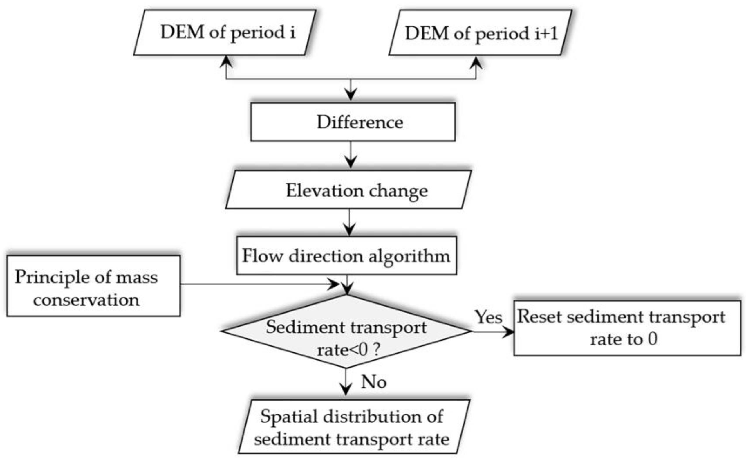
2.1. Algorithm Design

(1)

Simulation of the sediment transport process based on the SFD algorithm

In the SFD algorithm, the flow in the central cell and the received upstream flow only went to an adjacent downstream cell, which was determined by a specific algorithm. The D8 algorithm, also known as the maximum slope descent algorithm, is the most widely used SFD algorithm, with the flow mode flowing from the central cell to the neighboring cell with the greatest slope descent among the eight adjacent cells, which can be expressed as follows [26]:

$$max\left\{\left(Z_i-Z_k\right)/d\right\}; k=1,2,\dots ,8$$

(1)

where Z_i is the elevation of the central cell i and Z_k is the elevation of its adjacent cell k; d is the cell distance, which is defined as when the adjoining cell k is located in the east–west or north–south directions of the central cell i, d is equal to the cell size; when the adjacent cell k is located in the diagonal direction, d is equal to $\sqrt{2}$ times the cell size.

When previous works used the D8 algorithm for the STR simulation, it was considered that the downstream cell in the direction of the greatest decline in the slope would receive all the sediment from the upstream cell, ignoring the possibility of negative sediment (STR) values during propagation. Hence, the model is modified to judge in a real-time mode whether its STR is negative, and if it is negative, the STR is set to 0 to avoid the propagation of negative values.

$$Q_b^k=\left\{\begin{array}{cc}\hfill \left[Q_s+\rho \left(1-p\right)\Delta V_i\right]/t,& Q_s>0\hfill \\ \hfill 0 ,& Q_s\le 0\hfill \end{array}\right.$$

(2)

where $Q_b^k$ is the STR of the central cell i in the direction of the maximum slope drop; $Q_s$ is the amount of sediment transported from the upstream cell to the central cell i; p is the porosity; $\rho$ is the material density; in practical applications, $\rho \left(1-p\right)$ corresponds to the soil bulk weight; $\Delta V_i$ is the volume change at i; and t is the time interval.

(2)

Simulation of the sediment transport process based on the MFD algorithm

The D8 SFD algorithm simulates the conveyance path of water from a holistic perspective. From the confluence point, the water flows downstream according to the flow direction until it reaches the outlet and leaves the watershed. However, in plain areas, it is difficult to determine the direction of the maximum slope drop due to the flat terrain, and the simulated flow paths are unreasonable, resulting in many parallel river networks [27,28]. In reality, the water flow in one cell mostly flows to multiple downstream cells. Based on this premise, the MFD algorithm was proposed. Among them, the most widely used are the slope exponent MFD algorithm (MFD–se) and the maximum downhill slope MFD algorithm (MFD–md).

In the MFD–se algorithm, the water can flow to any adjacent downstream cell, and the amount of water assigned is determined by an exponential function of the slope, which is [21]:

$$d_k=\frac{tan S_k{}^{\alpha }\times L_k}{{{\displaystyle \sum }}_1^{8}tan S_k{}^{\alpha }\times L_k}; k=1,2,\dots ,8$$

(3)

where k is the ordinal number of the eight adjacent cells to the central cell i; d_k is the assignment of water flow from the central cell i to the kth neighboring cell; tan S_k is the slope; α is the index controlling the flow dispersion or concentration; when α is 1, the algorithm is the MFD, and when it is infinite, the algorithm is equivalent to the SFD; L_k is the contour length weighting factor of the kth neighboring cell, which is defined as 0, 1/2, and $\sqrt{2}$/4 when the kth neighboring cell is above the central cell, below the central cell, and located in the horizontal or vertical directions, and below the central cell with a diagonal direction, respectively.

Combined with Equation (3), the model is modified to judge in a real-time mode whether its STR is negative, and if it is negative, the STR is set to 0 to avoid the propagation of negative values. The improved equation is as follows:

$$Q_b^k=\left\{\begin{array}{cc}\hfill \frac{tan S_k{}^{\alpha } \times L_k}{{{\displaystyle \sum }}_1^{8}tan S_k{}^{\alpha } \times L_k}\times \frac{\left[Q_s + \rho \left(1 - p\right)\Delta V_i\right]}{t},& Q_s>0\hfill \\ \hfill 0 ,& Q_s\le 0\hfill \end{array}\right.$$

(4)

where $Q_b^k$ is the STR of any cell i to its neighboring direction k, $Q_s$ is the amount of sediment transported from surrounding cells to the current central cell, and $\rho \left(1-p\right)$ is the soil capacitance.

The principle of the MFD–md algorithm is similar to MFD–se, but the level of flow assignment differs. In the MFD–md, the maximum downslope gradient is selected as the topographic feature e to establish the flow assignment function f(e) instead of the index α that controls the dispersion or concentration of flow in the MFD–se equation, which is given by [29]:

$$d_k=\frac{tan S_k{}^{f\left(e\right)}\times L_k}{{{\displaystyle \sum }}_1^{8}tan S_k{}^{f\left(e\right)}\times L_k}, f\left(e\right)=\frac{e-e_{min}}{e_{max}-e_{min}}\times \left(10-1.1\right)+1.1$$

(5)

where e is the maximum downslope gradient, e_min and e_max are the minimum and maximum values of e in the region, respectively.

Combining Equation (5) and continuing to improve Equation (4), the final formula for calculating the STR is obtained as follows:

$$Q_b^k=\left\{\begin{array}{cc}\frac{tan S_k{}^{f\left(e\right)} \times L_k}{{{\displaystyle \sum }}_1^{8}tan S_k{}^{f\left(e\right)} \times L_k}\times \left[Q_s+\rho \left(1-p\right)\Delta V_i\right]/t,\hfill & Q_s>0\hfill \\ \hfill 0 ,& Q_s\le 0\hfill \end{array}\right.$$

(6)

Equations (2), (4), and (6) require the slope, so the first period of the DEM is used to calculate the slope. Additionally, the boundary sediment flux Q_s is needed to calculate the STR using the abovementioned three equations. If the boundary Q_s is unknown, the STR of the small watershed is calculated as the relative STR; if the boundary Q_s is known, the absolute STR can be calculated. The sediment flux at the boundary is zero, so all three equations can be used to calculate the absolute STR in the small watershed.

2.2. Evaluation of Model Performance

The simulation of the sediment transport process using the current flow direction algorithm possibly leads to a negative STR, contrary to the principle of mass conservation [30]. Moreover, negative STR values will keep spreading to the downstream area, causing extensive areas with negative STR values. With the proposed improved flow direction algorithm, no negative values exist in the simulation results. The evaluation method of model performance by the proportion of the negative area used in previous studies is not applicable to this paper [31,32]. Thus, the ratio of the positive STR area to the whole sample area (P) can be used to evaluate the effect of the flow direction algorithm, and the formula is:

$$P=A_{positive}/A_{watershed}$$

where A_positive denotes the area of the region with positive STR values, A_watershed is the watershed area.

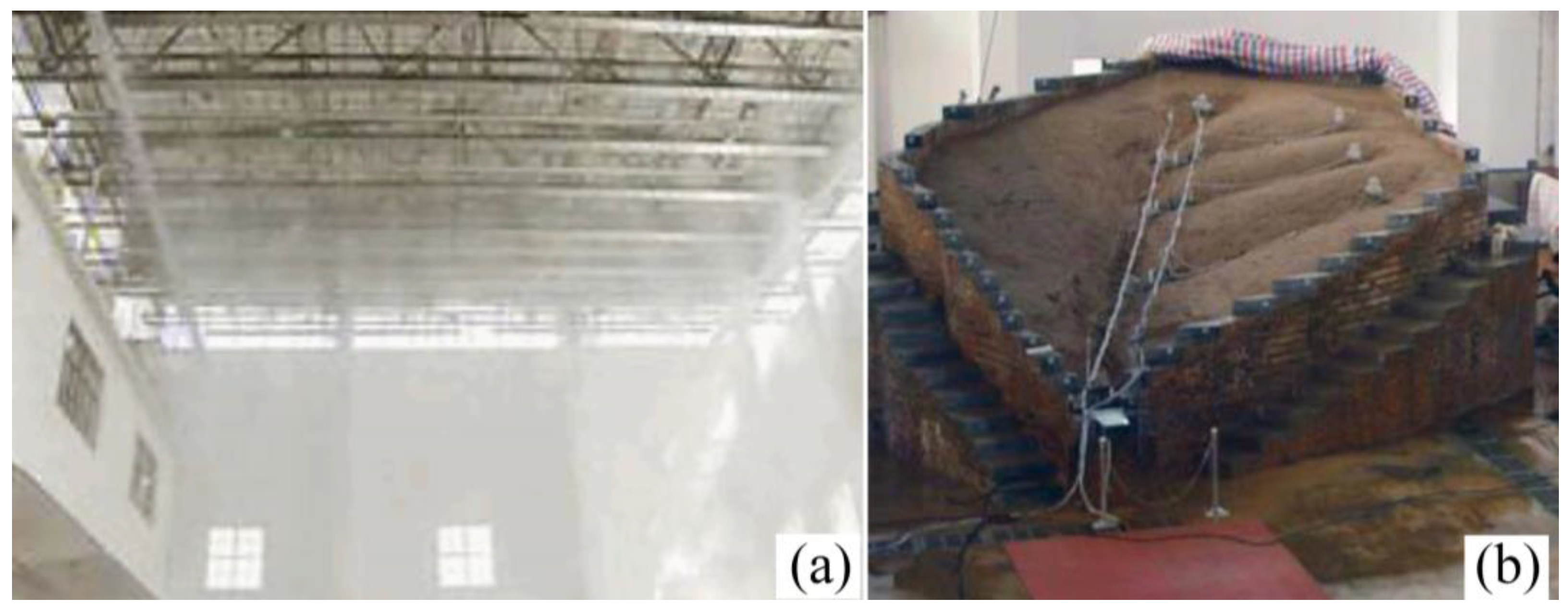
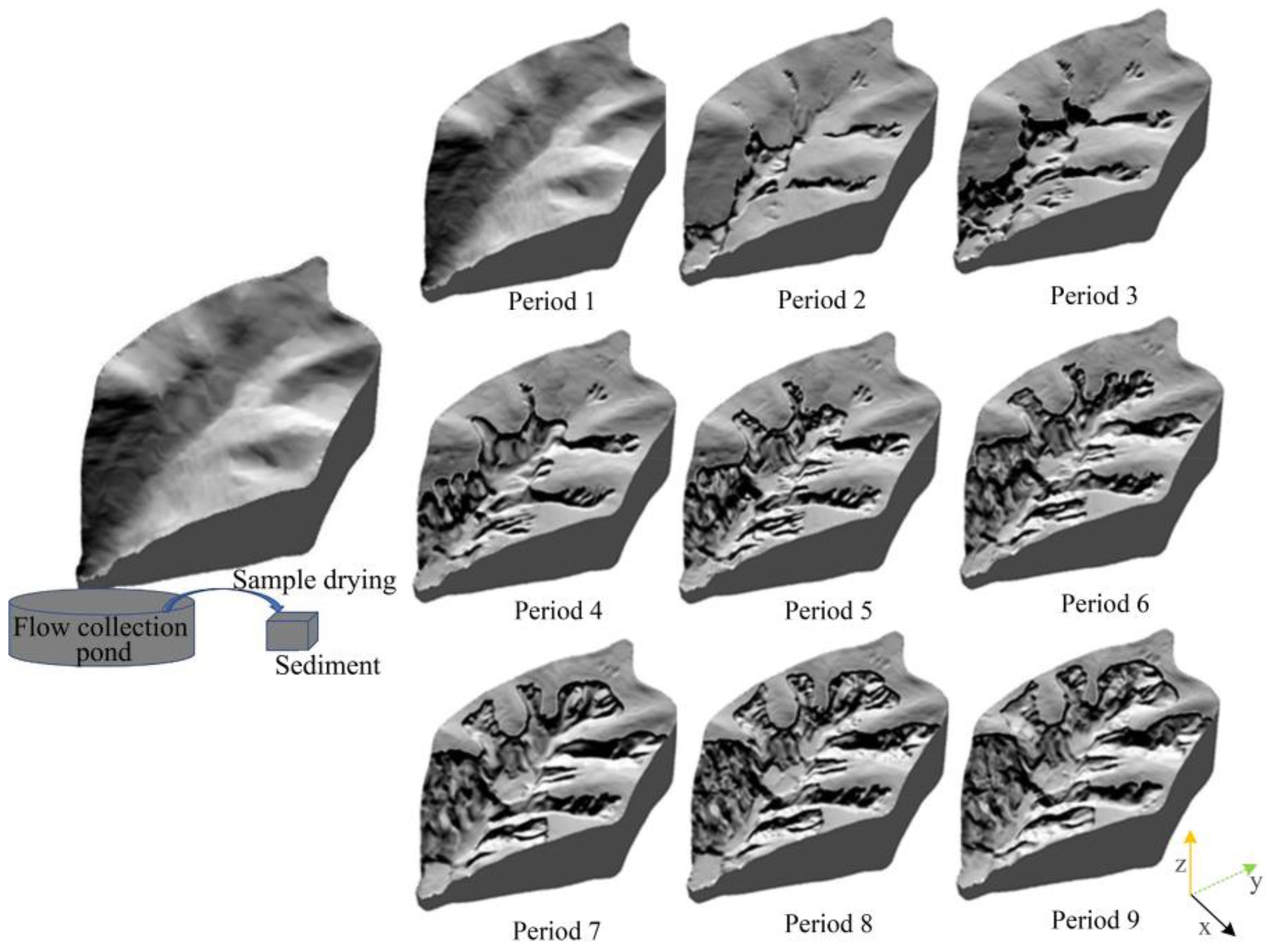
2.3. Experimental Sample Area and Data

This paper used an indoor simulated small watershed as the study area, and its basic morphological characteristics are shown in

Table 1. Basic properties of the simulated small watershed.

Aera	Length	Max Width	Perimeter	Height Difference	Longitudinal Gradient	Mean Slope	Soil Bulk Density
31.49 m2	9.1 m	5.8 m	23.3 m	2.57 m	28.24%	15°	1.39 g/cm3

. The experimental simulation in the study area was performed by the State Key Laboratory of Soil Erosion and Dryland Agriculture on the Loess Plateau [33]. The small watershed was composed of soil fill, compacted every 5 cm so that the soil capacity of each layer ranged from 1.36 to 1.4 g/cm³, with an average soil capacity of 1.39 g/cm³, where the median soil particle size was 0.005 mm.

The topography of the filled, indoor, small watershed was simulated for surfaces that were not eroded into gullies by rainfall. The simulated rainfall equipment and the simulated small watershed are shown in Figure 2. In the simulation experiment, 25 simulated rainfall events were conducted over 2.5 months after the simulated small watershed was constructed. The designed rainfall intensities were 0.5, 1, and 2 mm/min, representing small, medium, and heavy rainfall intensities in the Loess Plateau, which accounted for 44%, 36%, and 20% of the designed rainfall events, respectively. The different rainfall intensities were designed to simulate rainfall characteristics in realistic environments. The related runoff data were obtained during each rainfall event using a flow collection pond to calculate the rainfall volume at the watershed outfall. Additionally, the sediment in the flow collection pond was sampled, dried, and weighed during each rainfall event, and the average STR was calculated for each rainfall event. The hydrological monitoring data, such as the average rainfall intensity, cumulative rainfall duration, and average STR for each topographic measurement period, are shown in

Table 2. Monitored data of simulated small watershed.

Period	Rainfall Number	Rainfall Intensity (mm/min)	Rainfall Duration (min)	Rainfall Level (mm)	Mean STR at the Outlet (kg/min)
DEM1	1	0.54	90.5	48.87	1.86
	2	0.52	89.5	46.54	1.11
	3	0.49	89.5	43.86	1.73
	4	1.18	47.52	56.07	5.11
	5	1.21	45.86	55.49	14.07
DEM2	6	2.41	30.53	73.58	26.12
	7	1.19	46.17	54.94	13.88
DEM3	8	0.57	90.18	51.40	7.52
	9	0.59	61.95	36.55	7.81
DEM4	10	1.20	47.92	57.50	17.82
	11	2.15	31.17	67.02	35.97
DEM5	12	0.52	62.94	32.73	5.23
	13	0.58	61.53	35.69	6.02
	14	0.56	60.83	34.06	4.26
DEM6	15	1.12	46.82	52.44	10.98
	16	1.08	45.83	49.50	9.63
	17	0.98	47.02	46.08	7.97
	18	1.04	45.37	47.18	6.45
DEM7	19	2.12	30.37	64.38	16.73
	20	1.98	34.35	68.01	13.70
DEM8	21	0.53	91.27	48.37	3.01
	22	0.55	90.60	49.83	2.58
	23	0.60	89.72	53.83	2.83
DEM9	24	1.05	61.35	–	–
	25	2.03	31.65	–	–

.

Throughout the simulation process, 9 topographic measurements were completed using digital photogrammetry after rainfall events 5, 7, 9, 11, 14, 18, 20, 23, and 25, respectively, and 9 periods of DEM data were obtained with a resolution of 10 mm (Figure 3). The JPL Carl Zeiss SMK 120 stereo photogrammetry camera was used, and the JX–4 digital photogrammetric workstation from the Beijing Geo-vision information technology company was employed to generate the nine-period DEM data. The quality of the DEM was evaluated using 20 independent checkpoints, and it was calculated that the medium error in elevation was less than 2 mm for each period of the DEM. Specifically, the vertical mean errors of the DEM data for each period ranged from −0.09 to 0.28 mm, and the standard deviation ranged from ±1.64 to −1.98 mm. It should be noted that, in the subsequent analysis, the collection errors of the nine-period DEM data were negligible. Since topographic changes were significant over different periods employing the DEM, the number of topographic changes was on the level of centimeters, and the data collection error for the simulated small watershed was very low (2 mm), much lower than the level of the topographic change.

To analyze the connection between the topographic changes and rainfall data, runoff data, etc., hydrological monitoring data, such as the average rainfall intensity, cumulative rainfall duration, and average STR for each topographic measurement period, were required to be calculated, and the results are shown in Table 2.

3. Results

3.1. Analysis of the Improvement Effect of the SFD Algorithm

The simulation results of the sediment transport paths based on the D8 SFD model are shown in Figure 4, where the rainbow-colored bands from red to blue represent the magnitude of the STR. The grid scale used for showing the simulated results in the figure is 100 cm × 100 cm to present information on the length and width of the simulated small watershed and the relative spatial location of the STR in the watershed. In the SFD algorithm, the sediment in a grid cell could only flow to, at most, one grid cell, and the sediment transport direction was easily concentrated in one order, thus forming a parallel river network effect. Especially in the first three periods, because the gullies in the study area were not developed, the direction of the maximum elevation drop between neighboring grid cells was basically the same. Hence, the sediment transport paths were straight or nearly straight lines. With the development of gullies, this parallel river network effect diminishes, as in periods 7 and 8. Moreover, it can be observed that, before the improvement of the D8 algorithm, there are relatively many areas with negative STR values in the simulated watershed.

The negative values entirely disappear in the improved D8 SFD algorithm results (Figure 5). The indicators in the simulation results of the STR before and after the improvement are shown in

Table 3. Statistical information of each period before and after the D8 algorithm improvement.

		Period 1	Period 2	Period 3	Period 4	Period 5	Period 6	Period 7	Period 8
D8	Max	7470.44	8397.05	35,344.23	44,611.56	10,894.10	22,376.86	18,787.41	26,478.01
	Min	15.00	14.32	74.02	96.99	31.03	52.28	41.26	60.29
	Mean	0.25	0.22	0.87	1.22	0.15	0.40	0.48	0.54
	PPA	33.60%	33.51%	35.66%	37.10%	25.44%	38.49%	35.72%	40.77%
	PNA	0.00%	1.00%	4.48%	1.49%	10.93%	5.71%	8.29%	7.86%
Improved D8	Max	7470.44	8471.36	37,217.53	44,816.52	12,479.17	22,969.26	20,806.58	28,824.86
	Min	15.00	14.79	84.43	99.86	45.57	58.42	52.90	72.67
	Mean	0.25	0.23	1.13	1.31	0.42	0.53	0.71	0.76
	PPA	33.60%	33.83%	36.37%	37.57%	27.43%	40.19%	38.31%	43.05%
	PNA	0.00%	0.00%	0.00%	0.00%	0.00%	0.00%	0.00%	0.00%

Note: PPA: percentage of positive area; PNA: percentage of negative area.

. As can be seen, after the improvement, the maximum, mean, and median values increase due to the increase in the positive value region, and the rise in the proportion of the positive value region ranges from 0.00% to 2.59%, with a mean value of 1.26%. The improvement in the proportion of positive regions reflects the enhanced performance of the improved D8 algorithm. It is also clear from Table 3 that the improved D8 algorithm does not modify all the negative areas of the results simulated by the unimproved D8 algorithm to positive regions, and some of them are 0. Therefore, for the D8 algorithm, the improvement has some optimizations, but there are still some limitations.

The results of the improved D8 algorithm subtracted from the before-improved results show very few negative regions in the comparison results (Figure 6), and only positive areas appear to be present. This indicates that the improved D8 algorithm significantly improves the negative regions. It can be found that the areas with significant improvements are located in the downstream and centerline areas of the gully and part of the gully sidewall. The presence of more negative areas in the upstream region can be observed, and the STR accumulates in the process of propagating downstream. Thus, large, negative areas appear in the downstream region. Additionally, the propagated negative STR is heavily accrued at the centerline of the gully due to the fast flow rate.

3.2. Analysis of the Improvement Effect of the MFD Algorithm

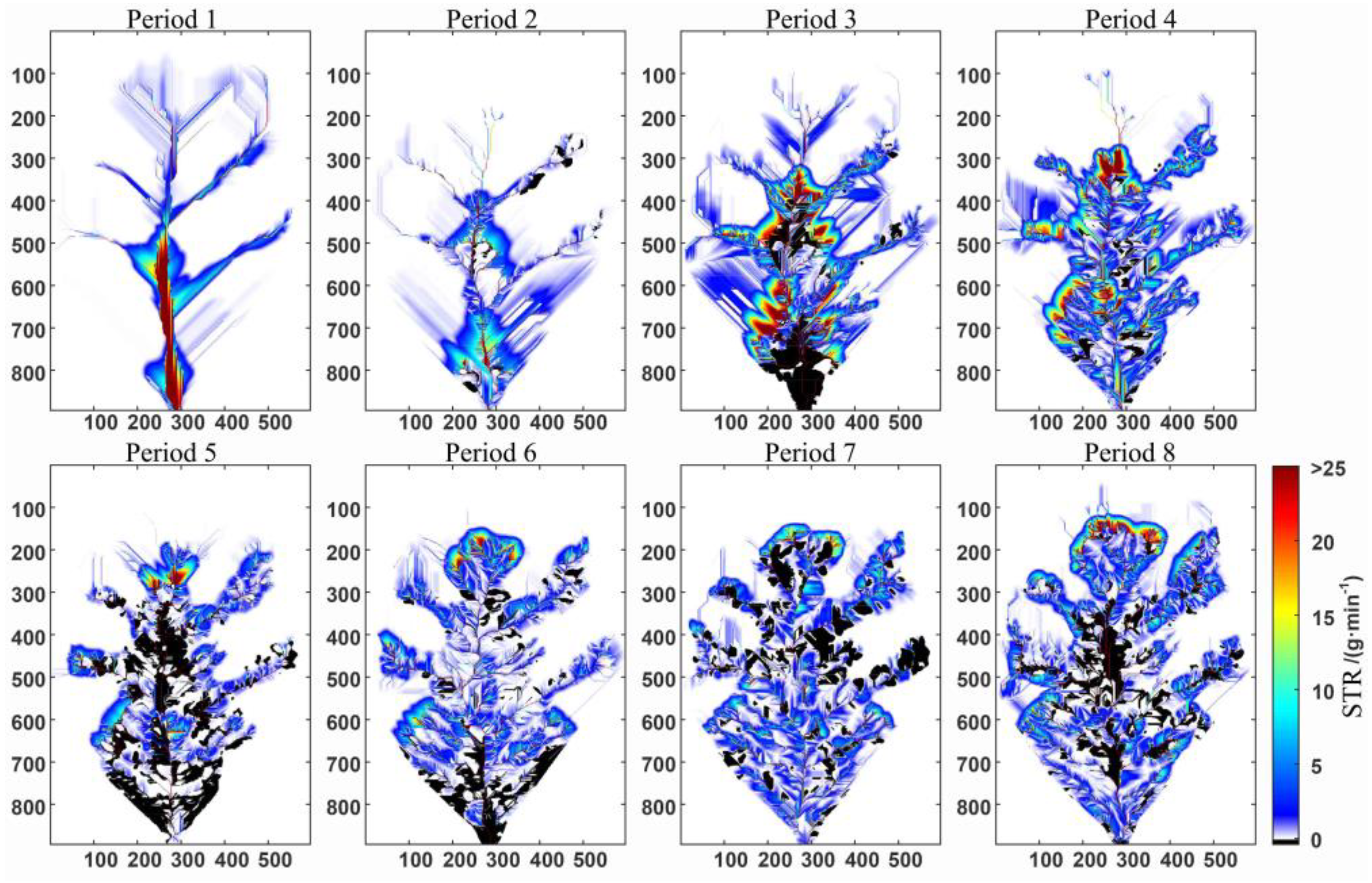
3.2.1. Simulation of the Sediment Transport Process Based on the MFD–se Algorithm

The simulation results of the sediment transport paths based on the MFD–se algorithm are shown in Figure 7, where the rainbow-colored bands from red to blue represent the magnitude of the STR. It can be observed that there are more areas with negative STRs in the watershed, especially in the fifth and seventh periods. The MFD algorithm allows sediment to flow from one grid cell to multiple grid cells downstream. Therefore, the MFD–se algorithm significantly improves the parallel river network effect of the simulation results compared to the SFD algorithm. The fact that sediment flow from the grid cells is no longer concentrated in one downstream grid also makes the path concentration effect of sediment transport less pronounced. As branch gullies develop, the sediment remains concentrated in the gullies, not just on the centerline, but throughout whole gullies, and this phenomenon is significantly more factual.

Figure 8 shows the simulation results of the improved MFD–se algorithm for the STR. The improved MFD–se algorithm significantly corrects the occurrence of negative STR values, with the negative region completely eliminated. The indicators of the results simulated by the MFD–se algorithm are shown in

Table 4. Statistical information for each period before and after the MFD–se algorithm improvement.

		Period 1	Period 2	Period 3	Period 4	Period 5	Period 6	Period 7	Period 8
MFD–se	Max	3815.63	7207.58	35,378.31	39,770.87	10,894.10	20,285.19	17,331.12	26,474.16
	Min	8.71	9.90	52.61	69.77	21.31	44.09	34.36	50.44
	Mean	0.04	0.10	0.50	0.63	0.02	0.33	0.36	0.55
	PPA	60.36%	52.17%	55.48%	54.75%	45.20%	49.54%	47.41%	55.62%
	PNA	0.00%	0.72%	3.08%	1.22%	10.30%	5.51%	8.27%	5.44%
Improved MFD–se	Max	3815.63	7256.98	36,211.57	39,822.40	12,006.44	20,582.70	19,034.43	27,676.04
	Min	8.71	10.01	53.96	69.89	23.03	44.82	38.18	52.14
	Mean	0.04	0.11	0.53	0.64	0.05	0.36	0.43	0.58
	PPA	60.36%	52.89%	58.09%	55.97%	55.24%	54.89%	55.44%	61.00%
	PNA	0.00%	0.00%	0.00%	0.00%	0.00%	0.00%	0.00%	0.00%

. As can be noticed, after the improvement of the MFD–se algorithm, the maximum, mean, and median values increase due to the increase in the positive area, and the increase in the proportion of the positive area ranges from 0.00% to 10.04%, with a mean value of 4.17%. The improved MFD–se algorithm does not show negative regions, which significantly affects the improvement of the simulation results, especially in the fifth and seventh periods. The area of the negative region in the results of the MFD–se algorithm for these two periods reached 10.30% and 8.27%, respectively, representing the two periods with the greatest errors. From the statistical values of the indicators before and after the improvement, it is evident that the improvement of the MFD–se algorithm is noticeable.

A comparison of the STRs between the two periods was obtained by subtracting the results of the before-improved MFD–se algorithm from the results of the improvement period, and it can be seen that the comparison results are similar to those of the D8 algorithm (Figure 9). The presence of large positive areas in the comparison results leads to the impression that no negative values exist, but negative areas are indeed present; they are just fewer in size. The areas where improvements were more evident were located downstream and on the centerline of the watershed and some of the watershed sidewalls. The continuous downward propagation of the negative STR results in many negative STR areas in the downstream area, similar to the improved results of the D8 algorithm. The difference is that there are more red areas in the comparison results of the MFD–se algorithm, which indicates that the difference between the MFD–se algorithm before and after the improvement is more remarkable. The improvement effect is more evident than that of the D8 algorithm.

3.2.2. Simulation of the Sediment Transport Process Based on the MFD–md Algorithm

The simulation results of the sediment transport paths based on the MFD–md algorithm are shown in Figure 10, where the rainbow-colored band from red to blue represents the magnitude of the STR. The results of the MFD–md algorithm are similar to those of the MFD–se algorithm due to the weighted assignment of flows, and the “parallel river network” effect and the concentration of sediment transport paths in the D8 algorithm are attenuated. Moreover, areas with negative STR values exist, especially the most obvious ones in the fifth and seventh periods.

The negative STR values entirely disappeared in the simulation results of the improved MFD–md algorithm (Figure 11). The indicators of the results simulated by the MFD–md algorithm are shown in

Table 5. Statistical information for each period before and after the MFD–md algorithm improvement.

		Period 1	Period 2	Period 3	Period 4	Period 5	Period 6	Period 7	Period 8
MFD–md	Max	4740.49	8289.73	35,364.24	39,675.66	10,894.87	22,139.55	16,562.19	26,480.26
	Min	8.38	9.44	50.72	68.95	20.62	42.21	32.63	48.03
	Mean	0.03	0.08	0.41	0.58	0.01	0.27	0.29	0.40
	PPA	60.34%	51.71%	54.37%	52.95%	44.21%	49.07%	47.00%	54.44%
	PNA	0.00%	0.79%	3.59%	1.33%	10.95%	5.73%	8.62%	6.59%
Improved MFD–md	Max	4740.49	8349.73	36,390.77	39,733.96	12,186.44	22,627.60	18,263.32	28,061.01
	Min	8.38	9.54	52.21	69.09	22.57	42.94	36.40	50.19
	Mean	0.03	0.08	0.43	0.59	0.03	0.29	0.34	0.42
	PPA	60.34%	52.51%	57.49%	54.28%	54.78%	54.63%	55.37%	60.98%
	PNA	0.00%	0.00%	0.00%	0.00%	0.00%	0.00%	0.00%	0.00%

. It can be observed that there are no longer any negative regions in the simulation results of the improved MFD–md algorithm, and the proportion of positive areas in each period has increased compared to that before the improvement, corresponding to increases in the maximum, mean, and median values. The increase in the proportion of positive regions ranges from 0.00% to 10.58%, with a mean value of 4.54%. After comparing the statistical indicator values of the calculation results of the MFD–se and MFD–md algorithms, it was found that the negative STR region calculated by the MFD–se algorithm was smaller than the MFD–md algorithm, indicating that the error of the MFD–se algorithm was lower and the simulation effect of the STR was better than that of the MFD–md algorithm.

3.2.3. Comparison of MFD–se and MFD–md Algorithms

To compare the differences between the simulations of STRs by the two algorithms, the simulation results of the MFD–se and MFD–md algorithms were subtracted correspondingly for each period to obtain the difference (Figure 12). The blue area is negative, indicating that the STR in this area in the simulation results of the MFD–se algorithm is lower than that in the simulation results of the MFD–md algorithm; the red area is positive, indicating that the STR in this area in the simulation results of the MFD–se algorithm is higher than that in the simulation results of the MFD–md algorithm. Sensorially, there are significantly more red than blue areas. Enlarging the difference diagram, it can be observed that the simulation results of the MFD–se algorithm are higher than those of the MFD–md in the part of the sidewall and gully (except the centerline). In contrast, at the centerline of the gully, the simulation results of the MFD–md algorithm are higher than those of the MFD–se algorithm. This indicates that the sediment distribution path of the MFD–md is more concentrated when simulating the sediment transport paths, so the STR is higher at the center line of the gully and lower at the sidewall and slope of the gully. This phenomenon is consistent with the flow distribution algorithm of the MFD–md algorithm. In practical applications, the MFD–md algorithm is more time-consuming and less efficient than the MFD–se algorithm. Consequently, the MFD–se algorithm is more suitable for the simulation of the STR.

4. Discussion

4.1. Influence of DEM Data Selection

As the primary data in the simulation of the sediment transport process, DEM data, with their derived parameters, such as slope and topographic change index, determine the effect of the STR simulation. When simulating the spatial distribution of the STR, the first-period DEM, the second-period DEM, or the mean values of these two DEM periods can be selected. To investigate the influence of DEM data selection on the sediment transport process, this paper obtained the DEM data of periods 1 and 2 as examples by using the better-performing MFD–se flow direction algorithm to simulate the spatial distribution of the STR. Figure 13 shows the percentage of areas with negative STRs using different DEMs. It was found that, when using the first-period DEM of each period, the proportion of the area with negative values of the STR was significantly smaller than the mean DEM and second-period DEM, indicating that it was more appropriate to use the first-period DEM to calculate the corresponding slope and other parameters in the STR simulation.

It is worth emphasizing that the topography changes gradually during erosion, and the sediment transport paths also continuously change. Thus, avoiding uncertainties in the path assignment calculation is difficult using only the period–1 DEM data. Moreover, as the topography changes become more evident over time, the uncertainty of the sediment transport path simulation using only the period–1 DEM increases. Despite the better performance of using the period–1 DEM in this experiment, using only the period–1 DEM for the STR simulation is theoretically not recommended. Another scenario worth discussing is the issue of topographic mutation points. In the process of topography change, there is probably such a mutation point where the terrain remains stable for a long enough time after the mutation point. Under this condition, the sediment is transported on this stable terrain for most of the time, and the sediment transport paths are significantly different from those under the first-period DEM, which is better with the period–2 DEM than with the period–1 DEM. In conclusion, the selection of DEM data is based on the actual topography change characteristics. In different cases, the stage of the topography change should be evaluated to select the appropriate DEM data.

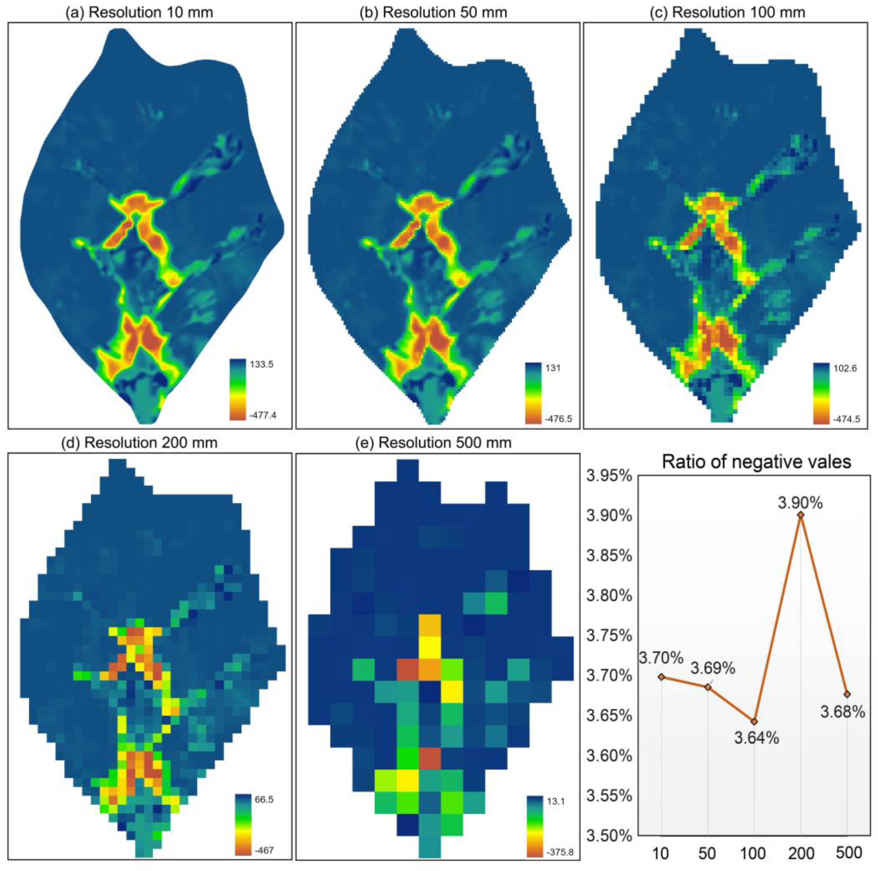
4.2. Influence of Spatial Resolution of the DEM Data

The scale effect is an inherent property for analyzing geographic issues, especially the uncertainty of the experimental results caused by data resolution [34,35]. In the proposed algorithm, the DEM resolution is an essential factor affecting the performance of the method. In this study, although processing high-resolution (10 mm) DEM data did not present the problem of an insufficient computer arithmetic, a high DEM resolution may have challenged the computer processing power when faced with large regional scales or large amounts of DEM data. In this case, an appropriate DEM resolution needed to be selected to balance the conflict between the data quality and computer arithmetic. Therefore, it is necessary to understand the variation of the DOD with a DEM resolution. To explore the effect of the DEM resolution on the spatial distribution of the STR and topographic changes, this paper used period–2 and –3 DEMs as examples and resampled the original DEM resolution (10 mm) to 50, 100, 200, and 500 mm to study the effect of DEM resolution on the DOD. The DOD was calculated by subtracting the period–2 DEM from the period–3 DEM [36]. Positive values signified material accumulation in the topography and negative values indicated the surface was eroded and material was lost. The results are shown in Figure 14. As can be seen, the decrease in the DEM resolution has little effect on the change in the proportion of negative values in the DOD. Moreover, the maximum value of the DOD change gradually decreases while the minimum value gradually increases. Meanwhile, the numerical variability of the DOD gradually decreases and the differentiation of the spatial distribution of negative values is gradually insignificant. It is evident that the higher the resolution of the DEM data, the higher the accuracy of the DOD calculation and the more apparent the topographic change characteristics.

Furthermore, the original resolution (10 mm) was resampled to 50, 100, 200, and 500 mm to observe the effect of the DEM resolution on the simulation of the spatial distribution of the STR, using the second-period DEM as an example. The experimental results are shown in Figure 15. As can be observed, with the gradual decrease in the DEM resolution, the spatial range of sediment transport becomes wider, and some slope areas without erosion transport are misjudged as having erosion transport, which leads to the overestimation of the STR in these areas. This suggests that a lower-resolution DEM causes misclassifications of STRs in areas without sediment transport and underestimates areas with inherently higher STRs. In addition to this local effect, the overall STR in the sample area (outlet STR) decreases with the coarser resolution of the DEM. Additionally, the use of a coarse-resolution DEM may also lead to abrupt changes in the STR in localized areas. For example, when using a 200 mm-resolution DEM, the STR at 350–400 cm downstream suddenly decreases extremely quickly. The reason for this phenomenon is that this area is the narrow gap in the channel (Figure 3), and due to the smoothing effect of a coarser DEM resolution, this “gap” is smoothed out, causing the sediment to get stuck in this part and not transported downstream.

Summarizing the variation of the STR spatial distribution with the DEM data resolution, it can be found that the effect of the STR simulation decreases with the quality of the DEM data, and coarser DEM data expand the sediment transport area and incorrectly calculate the value of the STR.

4.3. Analysis of the Reasons for a Negative STR

There are three possibilities for achieving a negative STR: one is caused by mass non-conservation due to measurement errors, the second is caused by incorrect flow direction algorithms, and the third is caused by anthropogenic disturbances. Suppose that a negative STR is caused by mass non-conservation due to measurement errors. In this case, it is theoretically reasonable to avoid this type of effect by assigning zero to the negative STR in this study. Suppose the flow direction algorithm generates a negative STR. In this case, this paper improves the flow direction algorithm by zeroing out the negative values, which somewhat affect the mass conservation. Yet, the overall STR in the negative area is relatively low (~0.01 kg/min), and the ratio is less than 0.01% compared to the total mass change (~100 kg). Correspondingly, the improved STR calculation results can be significantly optimized, with a maximum improvement of 10.95% from an area ratio perspective. It is considered acceptable to bring about more than a 10% optimization of the STR distribution area with an impact of less than a 0.01% loss of conservation of mass. The anthropogenic impacts did not need to be discussed in this paper since the study area was a simulated small watershed that excluded anthropogenic disturbances.

5. Conclusions

In the simulation of the sediment transport process based on the flow direction algorithm, the unreasonable flow direction algorithm caused the generation and propagation of negative STRs downstream, seriously affecting the simulation effect of the sediment transport process. This paper designed an improved flow direction algorithm for the sediment transport process simulation by judging the mass conservation situation in the simulation process, that is, whether the STR was negative or not, and if there was a negative STR, it was reset to 0 to stop the propagation of the negative STR downstream. The experimental results show that the performance of the improved D8 algorithm improves by 1.26% on average compared with that before the improvement, the performance of the improved MFD–se algorithm improves by 4.17% on average compared with that before the improvement, and the performance of the improved MFD–md algorithm improves by 4.54% on average compared with that before the improvement. Generally, the accuracy of the improved flow direction algorithms for the STR simulation results was improved, especially for the MFD algorithm. Meanwhile, comparing the three improved flow direction algorithms, it was found that the MFD–se algorithm was the most suitable for the simulation of the STR.

It is worth pointing out that we did not target the improvement of the common flow direction algorithm. Instead, we oriented the improvement of the flow direction algorithm for specific sediment transport process scenarios, thus providing a more reasonable calculation of the STR. Consequently, the proposed method can be applied to scenarios related to sediment transport processes, such as soil erosion control, soil and water conservation monitoring, and agricultural production management. It can also provide methodological references for the related research. With the development of UAV photogrammetry, radar surveying, and other technologies, it is increasingly convenient to obtain high-precision topographic data. The applicability of the proposed improved flow algorithm on the field measurement of high-precision topographic data will continue to be explored in future research. Additionally, in natural basin systems, when anthropogenic factors alter the topography, there is a lack of conservation of mass, and consequently, a negative STR occurs. Thus, the negative region of the STR can be considered in subsequent studies to measure the intensity of anthropogenic surface modifications.

References

1. Orlandini, S.; Moretti, G. Determination of Surface Flow Paths from Gridded Elevation Data. Water Resour. Res. 2009, 45, W03417. [Google Scholar] [CrossRef]
2. Chorowicz, J.; Ichoku, C.; Riazanoff, S.; Kim, Y.-J.; Cervelle, B. A Combined Algorithm for Automated Drainage Network Extraction. Water Resour. Res. 1992, 28, 1293–1302. [Google Scholar] [CrossRef]
3. Shin, S.; Paik, K. An Improved Method for Single Flow Direction Calculation in Grid Digital Elevation Models. Hydrol. Process. 2017, 31, 1650–1661. [Google Scholar] [CrossRef]
4. Scarpa, G.M.; Braga, F.; Manfè, G.; Lorenzetti, G.; Zaggia, L. Towards an Integrated Observational System to Investigate Sediment Transport in the Tidal Inlets of the Lagoon of Venice. Remote Sens. 2022, 14, 3371. [Google Scholar] [CrossRef]
5. Han, X.; Liu, J.; Mitra, S.; Li, X.; Srivastava, P.; Guzman, S.M.; Chen, X. Selection of Optimal Scales for Soil Depth Prediction on Headwater Hillslopes: A Modeling Approach. CATENA 2018, 163, 257–275. [Google Scholar] [CrossRef]
6. Tarboton, D.G. A New Method for the Determination of Flow Directions and Upslope Areas in Grid Digital Elevation Models. Water Resour. Res. 1997, 33, 309–319. [Google Scholar] [CrossRef]
7. Zhao, F.; Xiong, L.; Zhang, C.; Wei, H.; Liu, K.; Tang, G. Hydrological Object-Based Flow Direction Model for Constructing a Lake-Stream Topological System. Water Resour. Res. 2023, 59, e2022WR033681. [Google Scholar] [CrossRef]
8. Xiong, L.; Jiang, R.; Lu, Q.; Yang, B.; Li, F.; Tang, G. Improved Priority-Flood Method for Depression Filling by Redundant Calculation Optimization in Local Micro-Relief Areas. Trans. GIS 2019, 23, 259–274. [Google Scholar] [CrossRef]
9. Liu, X.; Wang, N.; Shao, J.; Chu, X. An Automated Processing Algorithm for Flat Areas Resulting from DEM Filling and Interpolation. ISPRS Int. J. Geo-Inf. 2017, 6, 376. [Google Scholar] [CrossRef]
10. Yamazaki, D.; Ikeshima, D.; Sosa, J.; Bates, P.D.; Allen, G.H.; Pavelsky, T.M. MERIT Hydro: A high-resolution global hydrography map based on latest topography dataset. Water Resour. Res. 2019, 55, 5053–5073. [Google Scholar] [CrossRef]
11. Lehner, B.; Grill, G. Global River Hydrography and Network Routing: Baseline Data and New Approaches to Study the World’s Large River Systems. Hydrol. Process. 2013, 27, 2171–2186. [Google Scholar] [CrossRef]
12. Jain, M.K.; Kothyari, U.C. Estimation of Soil Erosion and Sediment Yield Using GIS. Hydrol. Sci. J. 2000, 45, 771–786. [Google Scholar] [CrossRef]
13. Moore, I.D.; Wilson, J.P. Length-Slope Factors for the Revised Universal Soil Loss Equation: Simplified Method of Estimation. J. Soil Water Conserv. 1992, 47, 423–428. [Google Scholar]
14. Xia, Y.; Li, X.; Wang, T. A Hybrid Flow Direction Algorithm for Water Routing on DEMs. Acta Geod. Cartogr. Sin. 2018, 47, 683. [Google Scholar]
15. Xiong, L.; Tang, G.; Yan, S.; Zhu, S.; Sun, Y. Landform-oriented flow-routing algorithm for the dual-structure loess terrain based on digital elevation models. Hydrol. Process. 2014, 28, 1756–1766. [Google Scholar] [CrossRef]
16. Pei, T.; Qin, C.-Z.; Zhu, A.-X.; Yang, L.; Luo, M.; Li, B.; Zhou, C. Mapping Soil Organic Matter Using the Topographic Wetness Index: A Comparative Study Based on Different Flow-Direction Algorithms and Kriging Methods. Ecol. Indic. 2010, 10, 610–619. [Google Scholar] [CrossRef]
17. Zhang, H.; Shao, Z.; Sun, J.; Huang, X.; Yang, J. An Extended Watershed-Based AHP Model for Flood Hazard Estimation: Constraining Runoff Converging Indicators via MFD-Derived Sub-Watershed by Maximum Zonal Statistical Method. Remote Sens. 2022, 14, 2465. [Google Scholar] [CrossRef]
18. O’Callaghan, J.F.; Mark, D.M. The Extraction of Drainage Networks from Digital Elevation Data. Comput. Vis. Graph. Image Process. 1984, 28, 323–344. [Google Scholar] [CrossRef]
19. Freeman, T.G. Calculating Catchment Area with Divergent Flow Based on a Regular Grid. Comput. Geosci. 1991, 17, 413–422. [Google Scholar] [CrossRef]
20. Gallant, J.C.; Wilson, J.P. TAPES-G: A Grid-Based Terrain Analysis Program for the Environmental Sciences. Comput. Geosci. 1996, 22, 713–722. [Google Scholar] [CrossRef]
21. Quinn, P.; Beven, K.; Chevallier, P.; Planchon, O. The Prediction of Hillslope Flow Paths for Distributed Hydrological Modelling Using Digital Terrain Models. Hydrol. Process. 1991, 5, 59–79. [Google Scholar] [CrossRef]
22. Wang, Y.; Liu, X.; Li, J.; Wang, Y.; Bai, J.; Zhou, Z. Quantifying the Spatial Flow of Soil Conservation Service to Optimize Land-Use Pattern under Ecological Protection Scenarios. Front. Earth Sci. 2022, 10, 957520. [Google Scholar] [CrossRef]
23. Dai, W.; Xiong, L.; Antoniazza, G.; Tang, G.; Lane, S.N. Quantifying the Spatial Distribution of Sediment Transport in an Experimental Gully System Using the Morphological Method. Earth Surf. Process. Landf. 2021, 46, 1188–1208. [Google Scholar] [CrossRef]
24. Dietrich, W.E.; Smith, J.D.; Dunne, T. Flow and Sediment Transport in a Sand Bedded Meander. J. Geol. 1979, 87, 305–315. [Google Scholar] [CrossRef]
25. Dai, W.; Qian, W.; Liu, A.; Wang, C.; Yang, X.; Hu, G.; Tang, G. Monitoring and Modeling Sediment Transport in Space in Small Loess Catchments Using UAV–SfM Photogrammetry. CATENA 2022, 214, 106244. [Google Scholar] [CrossRef]
26. Jenson, S.K.; Domingue, J.O. Extracting Topographic Structure from Digital Elevation Data for Geographic Information-System Analysis. Photogramm. Eng. Remote Sens. 1988, 54, 1593–1600. [Google Scholar]
27. Lai, Z.; Li, S.; Lv, G.; Pan, Z.; Fei, G. Watershed Delineation Using Hydrographic Features and a DEM in Plain River Network Region. Hydrol. Process. 2016, 30, 276–288. [Google Scholar] [CrossRef]
28. Turcotte, R.; Fortin, J.-P.; Rousseau, A.N.; Massicotte, S.; Villeneuve, J.-P. Determination of the Drainage Structure of a Watershed Using a Digital Elevation Model and a Digital River and Lake Network. J. Hydrol. 2001, 240, 225–242. [Google Scholar] [CrossRef]
29. Qin, C.; Zhu, A.-X.; Pei, T.; Li, B.; Zhou, C.; Yang, L. An Adaptive Approach to Selecting a Flow-partition Exponent for a Multiple-flow-direction Algorithm. Int. J. Geogr. Inf. Sci. 2007, 21, 443–458. [Google Scholar] [CrossRef]
30. Hairsine, P.B.; Rose, C.W. Rainfall Detachment and Deposition: Sediment Transport in the Absence of Flow-Driven Processes. Soil Sci. Soc. Am. J. 1991, 55, 320–324. [Google Scholar] [CrossRef]
31. Antoniazza, G.; Bakker, M.; Lane, S.N. Revisiting the Morphological Method in Two-Dimensions to Quantify Bed-Material Transport in Braided Rivers. Earth Surf. Process. Landf. 2019, 44, 2251–2267. [Google Scholar] [CrossRef]
32. Bakker, M.; Antoniazza, G.; Odermatt, E.; Lane, S.N. Morphological Response of an Alpine Braided Reach to Sediment-Laden Flow Events. J. Geophys. Res. Earth Surf. 2019, 124, 1310–1328. [Google Scholar] [CrossRef]
33. Cui, L. The Coupling Relationship between the Sediment Yield from Rainfall Erosion and the Topographic Feature of the Watershed; Northwest A&F University: Xianyang, China, 2002. [Google Scholar]
34. Hengl, T. Finding the Right Pixel Size. Comput. Geosci. 2006, 32, 1283–1298. [Google Scholar] [CrossRef]
35. Wechsler, S.P. Uncertainties Associated with Digital Elevation Models for Hydrologic Applications: A Review. Hydrol. Earth Syst. Sci. 2007, 11, 1481–1500. [Google Scholar] [CrossRef]
36. Picco, L.; Mao, L.; Cavalli, M.; Buzzi, E.; Rainato, R.; Lenzi, M.A. Evaluating Short-Term Morphological Changes in a Gravel-Bed Braided River Using Terrestrial Laser Scanner. Geomorphology 2013, 201, 323–334. [Google Scholar] [CrossRef]
Figure 1. Workflow map.
Water 15 04111 g001
Figure 2. Photographs of the experimental environment: (a) simulated rainfall equipment and (b) simulated small watershed.
Water 15 04111 g002
Figure 3. Nine-period topographic data for the simulated small watershed [23].
Water 15 04111 g003
Figure 4. Results of the STR based on the D8 SFD algorithm.
Water 15 04111 g004
Figure 5. Results of the STR based on the improved D8 SFD algorithm.
Water 15 04111 g005
Figure 6. Comparison of STR results before and after the improvement based on the D8 algorithm.
Water 15 04111 g006
Figure 7. Results of the STR based on MFD–se algorithm.
Water 15 04111 g007
Figure 8. Results of the STR based on improved MFD–se algorithm.
Water 15 04111 g008
Figure 9. Comparison of the STR based on the before and after improvements of the MFD–se algorithm.
Water 15 04111 g009
Figure 10. Results of the STR based on the MFD–md algorithm.
Water 15 04111 g010
Figure 11. Results of the STR based on the improved MFD–md algorithm.
Water 15 04111 g011
Figure 12. STR comparison results between MFD–se and MFD–md algorithms.
Water 15 04111 g012
Figure 13. The proportion of areas with negative STRs under different DEM selections.
Water 15 04111 g013
Figure 14. The proportion of negative values in the DOD under different DEM resolutions.
Water 15 04111 g014
Figure 15. Effect of DEM resolution on the spatial distribution of the STR.
Water 15 04111 g015