Article

Dynamic Evolution and Copula-Based Multivariable Frequency Analysis of Meteorological Drought Considering the Spatiotemporal Variability in Northwestern China

1
Yinshanbeilu Grassland Eco-Hydrology National Observation and Research Station, China Institute of Water Resources and Hydropower Research, Beijing 100038, China
2
College of Water Conservancy, North China University of Water Resources and Electric Power, Zhengzhou 450045, China
3
State Key Laboratory of Eco-Hydraulics in Northwest Arid Region of China, Xi’an University of Technology, Xi’an 710048, China
*
Author to whom correspondence should be addressed.
Water 2023, 15(21), 3861; https://doi.org/10.3390/w15213861
Submission received: 16 September 2023 / Revised: 25 October 2023 / Accepted: 1 November 2023 / Published: 6 November 2023
(This article belongs to the Special Issue Drought Monitoring and Risk Assessment)

Abstract

:
Meteorological drought is a continuous spatiotemporal phenomenon that poses a serious threat to water resource security. Dynamic evolution and multivariable frequency analysis of meteorological drought are important for effective drought mitigation and risk management. Therefore, this study aims to analyze meteorological drought events in northwestern China between 1960 and 2018 based on the standardized precipitation evapotranspiration index (SPEI) through a three-dimensional identification method. This study investigates the meteorological drought dynamic evolution on different time and space scales and evaluates the frequency analysis considering the spatiotemporal variability based on Copula. The results show that SPEI presents an upward trend in Northwestern China. A trend towards increased humidity is observed in arid regions, contrasted by a trend towards aridification in semi-arid and semi-humid areas, indicating that the spatial distribution of drought in the study area tends towards homogenization. The possibility of high-intensity drought events occurring in the same area was relatively low, whereas low-intensity drought events were frequent. Additionally, this study analyzes the dynamic migration process of individual drought events from a three-dimensional perspective. Neglecting any one drought variable could significantly underestimate the occurring probability of severe drought events. Therefore, a multivariable frequency analysis considering the spatiotemporal variability plays a crucial role in the formulation of drought prevention and mitigation strategies, as well as drought forecasting.

1. Introduction

A meteorological drought is a water shortage phenomenon caused by an imbalance between the water supply and demand. It is prolonged by the decrease in precipitation below the climate-normal precipitation. A meteorological drought is one of the most serious natural disasters in the world. In recent years, drought has become a critical environmental problem, threatening human survival, and has aroused widespread concern in the scientific community. The IPCC report (https://www.ipcc.ch/ accessed on 24 October 2023) pointed out that the intensified global warming since the end of the 20th century has led to enhanced surface evaporation and significant regional differences in precipitation, further exacerbating the drought trend. It is therefore urgent to carry out an analysis on the spatiotemporal evolution characteristics and risk of drought to provide a scientific basis for regional drought prevention, drought resistance, and water resource management.
Drought indices can well reflect the wet and dry conditions. The research mechanisms of various drought indices are different, and their applicability in each region is also different. Therefore, an objective and reasonable selection of drought indices is of great practical significance to drought research. Scholars have proposed various drought indices, such as the Palmer Drought Severity Index (PDSI), the Standardized Precipitation Index (SPI), and the Standardized Precipitation Evapotranspiration Index (SPEI). Among them, PDSI is based on the principle of surface water balance to consider the water conditions in the early drought stage. The application of the PDSI is limited by its complex calculations, regional parameters, and single time scale. The SPI has the advantages of simple calculations and multiple time scales, but it ignores the role of temperature in drought formation. In the context of climate change, it is necessary to comprehensively consider the joint effects of precipitation and temperature in drought assessments. In view of this, the SPEI was proposed by Vicente-Serrano et al. [1], which combines the advantages of the PDSI and SPI and performs well in regional drought research.
Understanding the occurrence and spatiotemporal progression of drought is essential for formulating effective strategies to mitigate its impacts. Numerous studies have delved into the spatiotemporal features of drought, aiming to comprehend its characteristics on a regional scale. For example, Tong et al. [2] utilized the Standardized Precipitation Evapotranspiration Index (SPEI) to discern the fluctuations and trends of drought occurrences on the Mongolian Plateau, spanning the period from 1980 to 2014. Sun et al. [3] investigated the spatiotemporal evolution of the 2009–2011 meteorological drought in Southwest China based on the SPEI. Previous research on drought predominantly focused on spatial pattern analysis utilizing data accessible within the specified area [4]. For instance, statistical techniques such as correlation analysis and empirical orthogonal functions were employed to assess the regional attributes of drought occurrences [5,6,7]. Nevertheless, these approaches often simplify the three-dimensional (3D) structure of drought events by reducing the temporal and spatial information into one or two dimensions. For example, this includes examining the temporal changes of fixed-area drought indices or spatial distribution of drought conditions within a specific time frame [8]. In practice, drought events frequently exhibit evident heterogeneity and continuity across various time and space scales. As a result, drought characterization analysis in low-dimensional subspaces cannot well reflect the actual and continuous spatiotemporal evolution characteristics of drought events [9,10].
Copula functions have been widely applied in constructing multivariate joint probability distributions for drought analysis. Over the past few decades, there has been a significant increase in the use of Copula functions for multivariate drought frequency analysis [11,12]. For example, Lee et al. [13] employed Frank and Gumbel Copula functions for bivariate drought frequency analysis. Huang et al. [14] used Bayesian Copula as the best joint distribution function for probabilistic characterization analysis of dry-wet conditions. Ma et al. [15] constructed the trivariate joint distribution of drought duration, severity, and peak based on elliptical Copulas and symmetrical and asymmetrical Archimedean Copulas. Ma et al. [16] proposed the SDF relationships of streamflow drought in the source area of the Yellow River (SAYR) using a Copula-based approach. However, most of these studies focused on temporal features of drought, such as the duration and severity and failed to consider the drought-affected area in the frequency analysis. The spatial characteristics (e.g., drought-affected area) play an important role in characterizing the spatiotemporal structures of drought [17].
Located in the hinterland of the Eurasian continent, Northwestern China is one of the most arid regions at the same latitude and is also an ecologically fragile and climate-sensitive area. Its ecological environment, water resources, and socio-economic development are greatly impacted by regional climate change, and the regional climate responds significantly to global climate warming. Many studies in the 20th century believed that the climate in Northwestern China is generally warm and dry [18,19]. This is confirmed by the rapid retreat of glaciers, the significant degradation of vegetation and oases, the continuous disappearance of wetlands, and a significant reduction in lake areas [20]. In contrast to previous studies, some scholars in the early 21st century discovered that the northwest region has experienced a continuous increase in runoff since the mid-to-late 1980s [21,22]. Based on these findings, researchers proposed that the climate in Northwestern China may be transitioning from warm-dry to warm-wet, with the transition well underway in the western region. Although there has been a certain level of precipitation increase in the western region since the mid-to-late 1980s, the eastern region has experienced a decrease in precipitation.
Therefore, this paper uses the SPEI to study the spatial-temporal patterns and multivariate frequency characteristics of drought in northwest China over the past 60 years. By analyzing the warm-wet and warm-dry patterns in this region, this paper aims to provide a scientific decision-making basis for regional drought prevention, drought resistance, and disaster reduction. The results have important practical significance for understanding the dynamic evolution of drought in northwest China under climate change.

2. Materials and Methods

2.1. Study Area

The study area encompasses Northwestern China, including the three provinces of Shanxi, Gansu, and Qinghai, as well as the Ningxia Hui Autonomous Region and the western portion of the Inner Mongolia Autonomous Region (Figure 1). This region is situated between longitudes of 89°25′~111°27′ E and latitudes of 31°33′~42°48′ N. It covers an approximate land area of 1.87 million km2, accounting for roughly 19.46% of the total area in China. The elevation ranges from 184 to 6672 m, exhibiting significant spatial variation with a decrease from west to east. The study area has a diversified topography of mountains, plateaus, and basins, presenting as the Qinghai-Tibet Plateau, Gobi desert, desert steppe, and Loess Plateau from west to east [23].
The study area is mainly affected by the westerlies, Asian monsoons, and plateau monsoons, resulting in dry and cold winters and wet and hot summers [24]. The annual precipitation varies from 50 to 900 mm. The majority of rainfall occurs between June and September, contributing to around 72% of the total annual precipitation. The annual potential evapotranspiration ranges from approximately 800 to 1600 mm, displaying notable spatial diversity and a descending trend from north to south. The mean annual temperature is around 9 °C [25].

2.2. Dataset

In recent years, satellite remote sensing data has been widely applied in Earth science research due to their long time-series, extensive coverage, and high applicability [25]. In this study, monthly precipitation (P) and potential evapotranspiration (PET) data from the CRU TS v.4.03 dataset (https://crudata.uea.ac.uk/cru/data/hrg/ accessed on 18 August 2023) are employed to compute the Standardized Precipitation Evapotranspiration Index (SPEI). The time series covers the years from 1960 to 2018, with a spatial resolution of 0.5° × 0.5°. Additionally, monthly meteorological data of 70 observation stations in the study area obtained from the National Meteorological Information Center are utilized to assess the accuracy of the remote sensing dataset. It is observed that over 85% of the observation stations in the study area exhibited the determination coefficient (R²) values concentrated in the range of 0.7 to 0.9 (with a significance level of p = 0.01). This demonstrates a good consistency between the meteorological data from the observation stations and the CRU dataset [26,27].

2.3. Methods

2.3.1. Standardized Precipitation Evapotranspiration Index

The Standardized Precipitation Evapotranspiration Index (SPEI), developed by Vicente-Serrano [1], is effective for assessing drought conditions under climate change [28,29,30]. The SPEI reflects the drought situation at different time scales through the difference between precipitation and potential evapotranspiration (PET) [31]. The PET is calculated using the Penman-Monteith method, incorporating various climatic variables (e.g., temperature, rainfall, wind speed, and insolation), as shown in formula (1).
P E T = 0.408 × Δ × ( R n G ) + γ × 900 T + 273 × U 2 × ( e s e a ) Δ + γ × ( 1 + 0.34 × U 2 )
where ∆ is the slope of the saturation vapor pressure temperature relation curve, kPa/°C; Rn is the net amount of radiation reaching the ground, MJ/m2d; G is the soil heat flux density, MJ/m2d; γ is the hygrometer constant; U2 is the wind speed 2 m above ground level, m/s; es is the saturated water vapor pressure of air, kPa; and ea is the actual vapor pressure, kPa.
Then, the drought severity values of SPEI can be obtained via the following steps:
First, the difference series between precipitation and potential evaporation is given by
D n k = i = 0 k 1 ( P n i P E T n i )     n k
where P is the precipitation in a particular time scale; PET is the potential evapotranspiration on the same period; i is the month; n is the number of calculations; and k is the time scale for the calculations.
Second, the 3-parameter log-logistic probability distribution function is used to fit the Dnk series. The probability distribution function F(x) is
F ( x ) = [ 1 + ( α x γ ) β ] 1
where α is the scale parameter; β is the shape parameter; and γ is the positional parameter.
Third, the F(x) value is transformed to a standard normal distribution, and then, the SPEI can be calculated using
S P E I = W C 0 + C 1 W + C 2 W 1 + d 1 W + d 2 W 2 + d 3 W 3
where C0 = 2.5155, C1 = 0.8028, C2 = 0.0103, d1 = 1.4327, d2 = 0.1892, and d3 = 0.0013.
Table 1 presents the drought levels classified according to the SPEI. Negative SPEI values indicate that the climate condition is dry (drought), while positive SPEI values represent a wet climate condition, and SPEI values near zero refer to normal climate conditions. And 1–12 month time scale SPEIs have been calculated for analysis. Droughts are defined when the SPEI value is less than −0.5 in this study.

2.3.2. Modified Mann-Kendall Test (MMK)

The conventional Mann-Kendall test (MK) assumes that the temporal series are random and independent. However, in practice, the time series of meteorological elements often exhibit autocorrelation, which can potentially compromise the reliability of the test results [32]. To address this problem, the Modified Mann-Kendall (MMK) test has been developed, a more rational non-parametric method for assessing the variation in time series. This method effectively addresses autocorrelation within the time series, leading to more reliable trend test results [33]. In this study, the MMK method is applied to analyze the temporal variation trend of drought as well as its spatial distribution characteristics at the grid scale. For a detailed calculation process of the MMK method, please refer to the research of Wang et al. [34].
In terms of the trend statistic value (Z), a positive value indicates an upward trend in the SPEI time series, whereas a negative value indicates a downward trend. Additionally, if the absolute value of Z exceeds 1.64, 1.96, and 2.58, the change trend of SPEI time series is considered significant at the levels of p = 0.1, p = 0.05, and p = 0.01, respectively.

2.3.3. R/S Analysis

The R/S diagnostic method, a non-parametric statistical method, is commonly used to investigate the fractal features and long-term memory dynamics within the time series. Under the context of the R/S analysis, the Hurst index is utilized to predict future trends and reflect the prolonged persistence characteristics and degree of memory in the time series. The detailed steps for the R/S analysis are available in the study of Araujo and Celeste [35].
According to Zhang et al. [36], the Hurst index H ranges from 0 to 1. When 0 < H < 0.5, it signifies that the future trend of the SPEI time series is opposite to its past state, with stronger anti-persistence as H approaches 0. In the case of H = 0.5, it indicates that the SPEI time series is an independent random process with no correlation between the past and future changes. When 0.5 < H < 1, it indicates that the future trend of the SPEI time series maintains consistency with its past state, with stronger persistence as H approaches 1.

2.3.4. Identification of Drought Events by a 3D Clustering Method

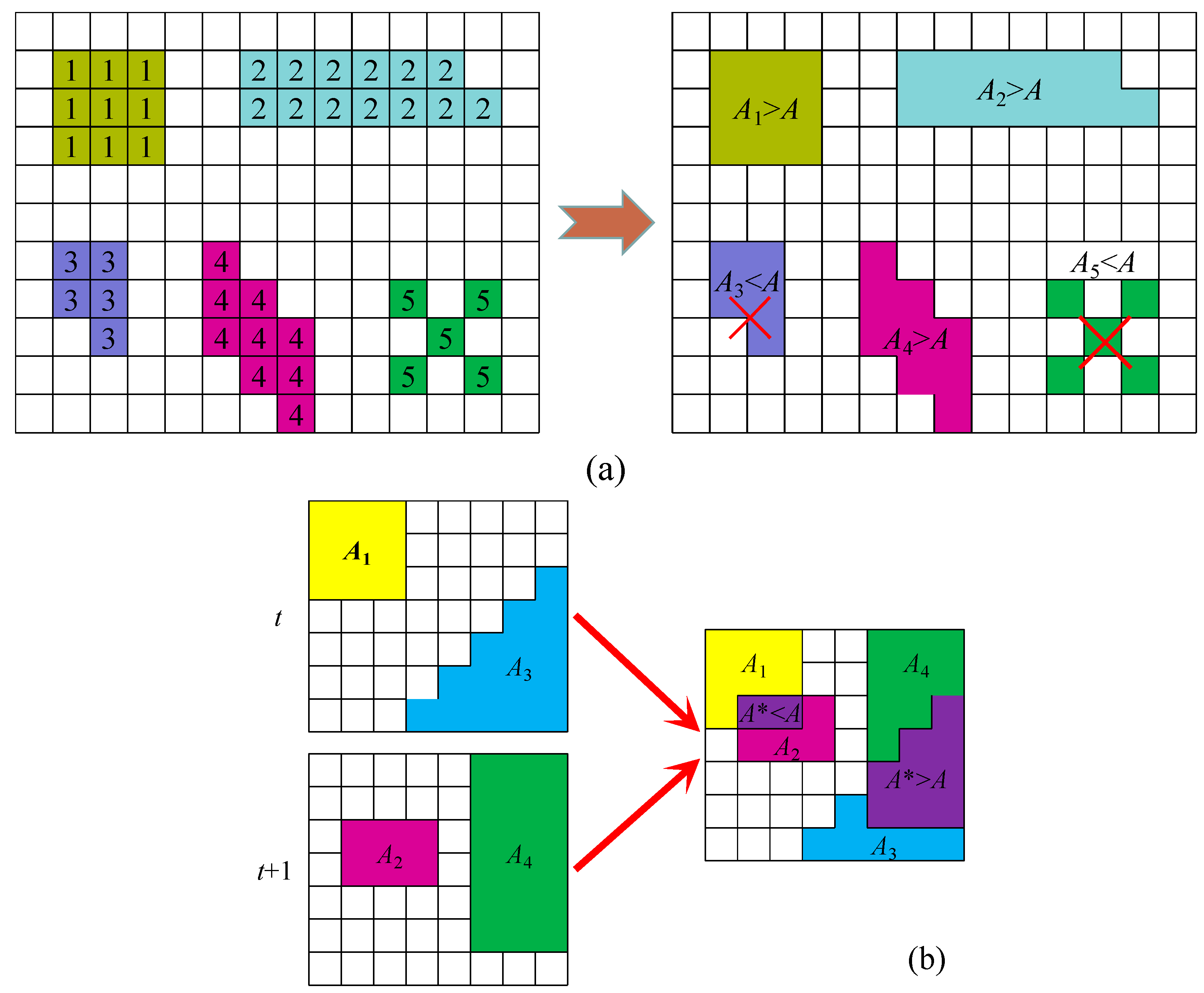
Drought identification is the precondition for evolution and frequency analysis of drought. Generally, drought events are characterized by spatial and temporal continuity (longitude, latitude, and time). It is therefore important to consider the spatiotemporal drought structure in the drought analysis [37,38]. In view of this, a 3D clustering method is used to identify the drought events and extract drought variables at different space-time scales. This method consists of two main steps: spatial identification of drought clusters and temporal connection of drought clusters (Figure 2). The detailed calculation process can be found in our previous research [12,25].
Based on the identification results, several spatiotemporal drought variables are defined and calculated. The definitions of these variables are as follows. Drought duration (D) refers to the time interval from the initiation to the termination of one event. Drought-affected area (A) represents the cumulative expanse impacted by a drought event throughout its entire duration. Drought severity (S) indicates the degree of the total water deficit during a drought episode, which is the volume of the three-dimensional drought structure. Drought intensity (I) represents the magnitude of drought in the study area, which can be reflected by the SPEI; the greater the absolute value of SPEI, the more severe the drought.

2.3.5. Copula-Based Multivariable Frequency Analysis of Drought Events

Marginal Distribution of Drought Variables

The accurate fitting of marginal distribution function of drought variables is the basis of the frequency analysis. Inaccuracies in fitting can lead to amplified errors in the calculation of joint distributions. Therefore, it is essential to precisely fit marginal distributions to drought variables. In this study, seven three-parameter distributions are considered [14,39,40]. Seven probability distribution functions, including Gamma, Log-logistic, Lognormal, Weibull, Pearson-III, Generalized Extreme Value, and Generalized Pareto distribution, are used to fit different drought variables. Table 2 shows the probability distribution function and related parameters.
In addition, the Kolmogorov-Smirnov (K-S) test is used to determine whether the assumed distribution significantly differs from the underlying distribution of the actual data at a significance level of p = 0.05. When p > 0.05 and the K-S statistic is below the critical value, it indicates that the assumed distribution agrees well with the underlying distribution of the drought variable. A smaller K-S statistic corresponds to a better fit of the distribution.

Determination of the Optimal Copula Function

The determination of the Copula function also greatly impacts the frequency analysis results of multivariate drought variables. Initially, the K-S method is used to assess whether alternative Copula functions pass the goodness-of-fit test. Subsequently, the relevance between alternative Copula functions and empirical Copula functions is measured using Root-Mean-Square Error (RMSE), Akaike Information Criterion (AIC), and Bayesian Information Criterion (BIC) [41]. The optimal Copula function is then determined based on the goodness-of-fit test results, which is used to establish the joint distribution among drought variables.
For simplicity and representativeness [42], six Copula functions are employed as candidate Copula functions. These include theoretical Archimedean Copulas (Frank, Clayton, Gumbel, and Joe) and elliptical Copulas (Normal and t) [43]. The estimation of Copula parameters was carried out through the inversion of Kendall’s (tau) method. Detailed information about the Copula functions is given in Table 3.

Copula-Based Multivariable Probability Calculation

It is assumed that D, S, and A are random variables, and the corresponding marginal cumulative distribution functions are denoted as FD(d), FS(s), and FA(a), respectively. The joint cumulative distribution function of drought variables based on optimal bivariate and trivariate Copula functions are as follows:
F ( d , s ) = P ( D d , S s ) = C ( F D ( d ) , F S ( s ) ) F ( d , a ) = P ( D d , A a ) = C ( F D ( d ) , F A ( a ) ) F ( s , a ) = P ( S s , A a ) = C ( F S ( s ) , F A ( a ) ) F ( d , s , a ) = P ( D d , S s , A a ) = C ( F D ( d ) , F S ( s ) , F A ( a ) )
The bivariate and trivariate joint occurrence probabilities are estimated under two distinct scenarios: (1) D and S (D and A, S and A, D and S and A) both exceed a specific threshold, denoted as P D S A a n d ; (2) either D or S (D or A, S or A, D or S or A) exceeds a given threshold, denoted as P D S A o r . The calculation formulas are as follows:
P D S a n d = P ( D > d S > s ) = 1 F D ( d ) F S ( s ) + C ( F D ( d ) , F S ( s ) )
P D S o r = P ( D > d S > s ) = 1 C ( F D ( d ) , F S ( s ) )
P D S A a n d = P ( D > d S > s A > a ) = 1 F D ( d ) F S ( s ) F A ( a ) + C ( F D ( d ) , F S ( s ) ) + C ( F D ( d ) , F A ( a ) ) + C ( F S ( s ) , F A ( a ) ) C ( F D ( d ) , F S ( s ) , F A ( a ) )
P D S A o r = P ( D > d S > s A > a ) = 1 C ( F D ( d ) , F S ( s ) , F A ( a ) )
The conditional drought probability plays an important role in water resource planning and management [40]. The detailed calculation process of conditional drought probability is as follows. For example, the expression for the conditional probability distribution of S > s given Dd is
F ( D d | S s ) = F ( D d , S s ) F ( S s ) = 1 F D ( d ) F S ( s ) + C ( F D ( d ) , F S ( s ) ) 1 F S ( s )
Similarly, the conditional distribution of D > d given Ss and Aa can be expressed as
F ( D d | S s , A a ) = F ( D d , S s , A a ) F ( S s , A a )   = 1 F D ( d ) F S ( s ) F A ( a ) + C ( F D ( d ) , F S ( s ) ) 1 F S ( s ) F A ( a ) + C ( F S ( s ) , F A ( a ) ) +   C ( F D ( d ) , F A ( a ) ) + C ( F S ( s ) , F A ( a ) ) C ( F D ( d ) , F S ( s ) , F A ( a ) ) 1 F S ( s ) F A ( a ) + C ( F S ( s ) , F A ( a ) )

3. Results

3.1. Spatial-Temporal Variation of Drought at Multiple Time Scales

3.1.1. Temporal Evolution Characteristics of Drought at Different Time Scales

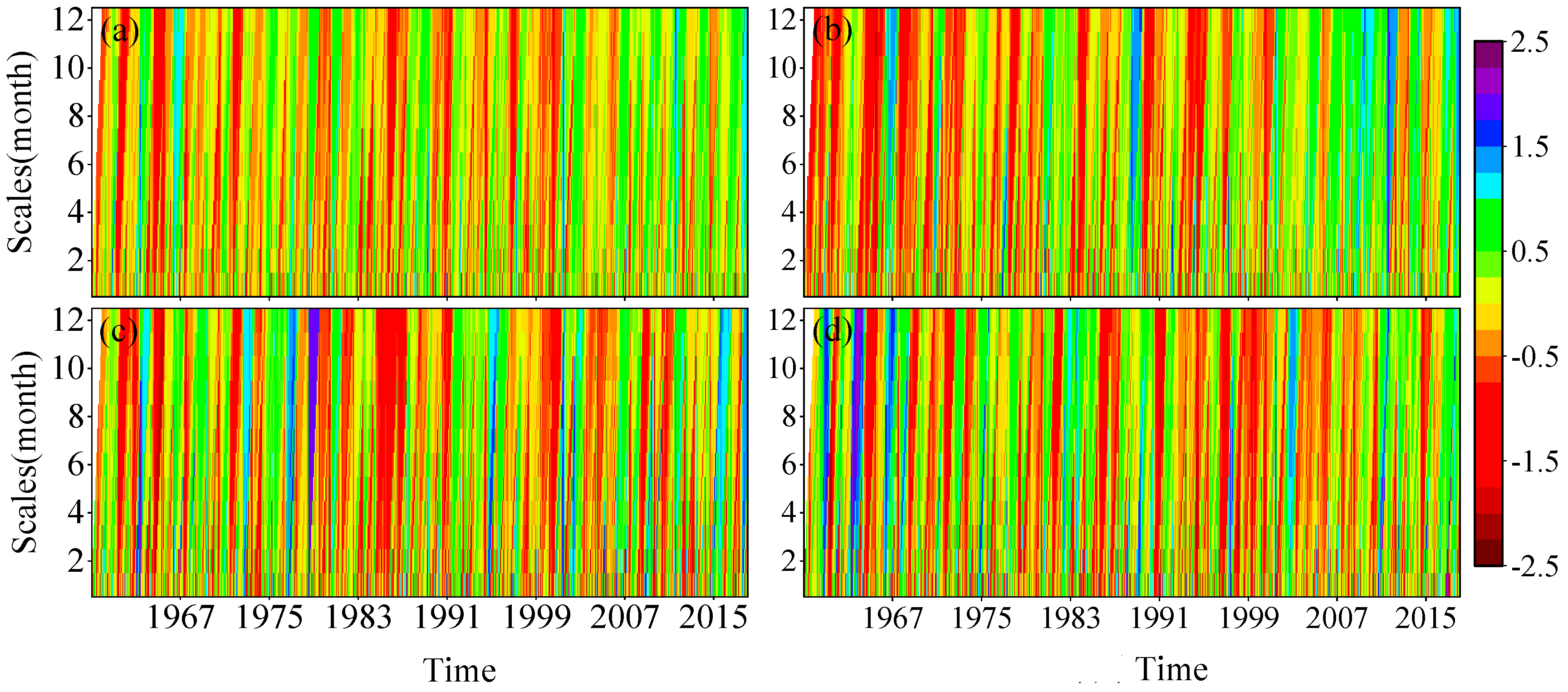
Figure 3 presents the temporal variation characteristics of the SPEI at the 1–12 month timescales in northwest China and its three climatic zones from 1960 to 2018. It can be observed that the meteorological drought was a gradual process in temporal evolution. With the increasing time scale, the drought variability declined, the inter-annual variation trend became more prominent, and the drought and wet cycles increased significantly. This implies that the frequency of drought decreased significantly, while the duration and intensity of drought increased. At different time scales, the SPEI in the plateau climate zone, westerly climate zone, and northwest China showed an ascending trend, indicating that droughts were abating (Figure 3a–c). However, the SPEI in the southeast climate zone presented a downward trend, indicating that droughts were aggravating (Figure 3d). The temporal variation characteristics of the SPEI in northwest China and the plateau climate zone were similar: a relatively severe meteorological drought occurred in around 1965; frequent droughts and floods alternated during the 1970–1990s; and drought events reduced significantly after 2005, with wet events dominating.
In the westerly climate zone, the 1970s was characterized by fluctuations in drought and flood. Drought and flood events alternated during this period. This region was dominated by drought events in the 1980s, with a severe and protracted drought from 1985 to 1988. In the 1990s, droughts significantly decreased with a decline in intensity. From the 2000s onward, drought and flood events fluctuated again, and droughts showed a deceasing trend. The drought trend in the southeast climate zone differed from that in other regions, with drought and flood events alternating until the 1990s, followed by a prolonged drought in the 1990s.

3.1.2. Spatial-Temporal Characteristics of Seasonal and Annual Drought Variation Trends

The variations in the SPEI at different time scales reflect its sensitivity to precipitation and temperature changes, as well as its cumulative effect over time. With the increasing time scale, the SPEI becomes more responsive to changes in precipitation and temperature, and short-term changes are less likely to affect its overall trend. Therefore, the SPEI is a reasonable indicator of long-term water variation.

Temporal Characteristics of Drought Variation Trend

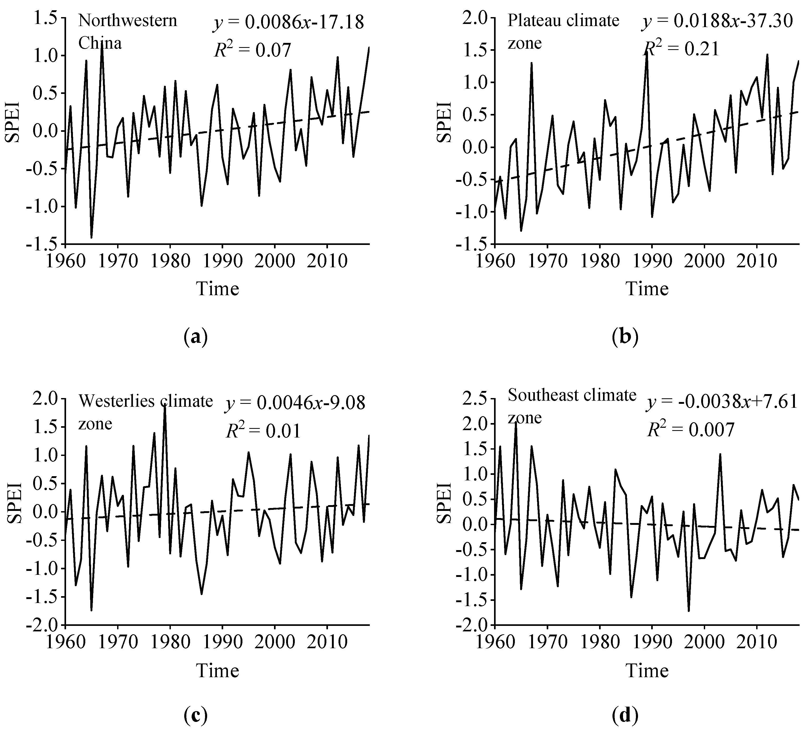
Figure 4 illustrates the annual variation in the SPEI in the northwest region from 1960 to 2018. It can be observed that the SPEI in the northwest region, plateau climate zone, and westerly climate zone all showed a fluctuating upward trend, indicating a trend towards increased moisture, with trend rates of 0.086/10a, 0.188/10a, and 0.046/10a, respectively. In contrast, the SPEI in the southeast climate zone showed a trend towards aridity, with a rate of −0.038/10a. Additionally, the variation trend of drought was particularly distinct in the plateau climate zone (R2 = 0.21).
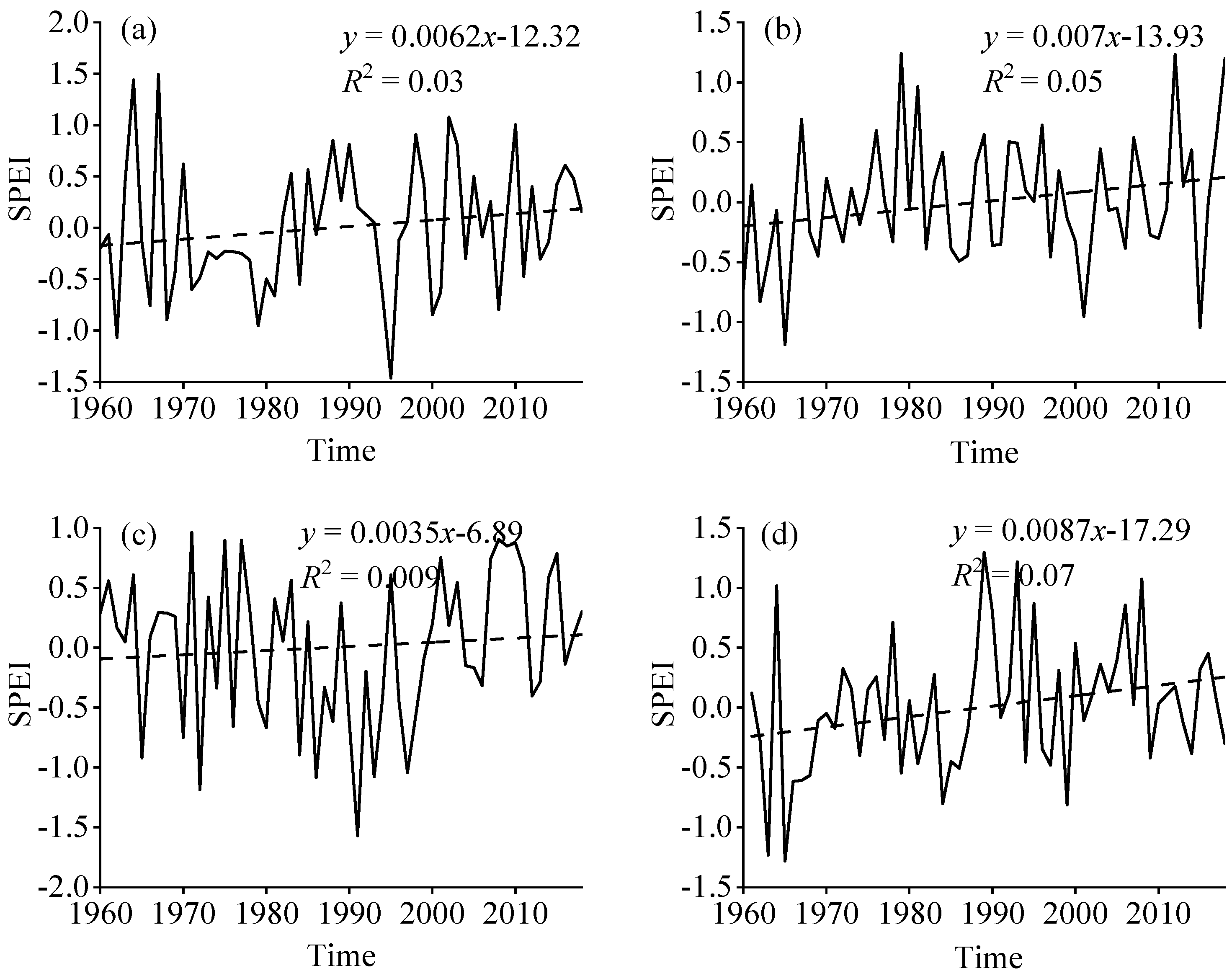
Figure 5 shows the seasonal variation in the SPEI in the northwest region from 1960 to 2018. Obviously, the SPEI in all four seasons showed a fluctuating upward trend during this period. According to the long-term trend analysis, the seasonal drought in the northwest region was decreasing, reflected as a trend towards increased moisture in all four seasons. The trend rates for spring, summer, autumn, and winter were 0.062/10a, 0.07/10a, 0.035/10a, and 0.087/10a, respectively. The interdecadal variation in the SPEI varied significantly among different seasons. In spring, the SPEI showed an upward trend in the 1960s, followed by a sharp decline in the 1970s, another ascending trend in the 1980s, and fluctuations thereafter, reaching its minimum in 1995 (−1.46). In summer, the SPEI showed a general upward trend in the 1960s and 1970s and a slight downward trend after 1980. Since then, it has been alternating between droughts and floods. In autumn, the SPEI was roughly on the decrease in the 1960s–1980s, indicating increased aridity, but shifted to an upward trend after 1990, indicating increased moisture. No drought events occurred after 2000. In winter, the SPEI showed an upward trend before 1975, followed by a downward trend in 1975–1985. After a brief upward trend from 1986 to 1990, it turned into a rapid downward trend in the 1990s. After 2000, the SPEI fluctuated up and down, but no drought events occurred. Based on the Z-index, Zhao et al. [44] analyzed the temporal and spatial characteristics of drought in northwest China. Their results showed that the Z-index of four seasons in northwest China showed an upward trend, with alternating droughts and floods and no obvious consistency among the seasons. This was consistent with the results of this study. In conclusion, the difference in climate conditions among the four seasons led to different SPEI variation characteristics in each season. Furthermore, the seasonal variation trends of the SPEI differed significantly from its annual variation trend.

Temporal Characteristics of Drought Variation Trend

The historical and future changes in seasonal SPEI in northwest China are reported in Table 4. According to the table, only the autumn SPEI in the southeast climate zone showed a decreasing trend, but the trend was not statistically significant. In the future, this index is likely to continue to decline, with a potentially high intensity of drought. The seasonal SPEI in the other regions showed a rising trend. Specifically, the spring and summer SPEIs in the northwest region and the winter SPEI in the southeast climate zone exhibited a statistically significant p-value of 0.1 for their ascending trends. In addition, the winter SPEI in the northwest region and the plateau climate zone showed a significant upward trend with a p-value of 0.05. Moreover, the spring and summer SPEIs in the plateau climate zone also showed an upward trend, with a statistically significant p-value of 0.01. These ascending trends appear to continue in the future, which indicates continuous moisture. Nevertheless, the upward trends of other SPEIs were not statistically significant. The spring and winter SPEI in the westerly climate zone, as well as the spring SPEI in the southeast climate zone, are likely to decline in the future, indicating the possibility of a low-intensity drought.
The characteristic value Z for the SPEI trend of each month is shown in Figure 6. The Z-values in the northwest region from January to December were 0.81, 0.28, −0.20, −0.11, 1.19, 1.8, 0.59, −0.25, 0.52, 0.14, −0.19, and 0.73. Among them, the SPEI for March, April, August, and November presented a decreasing trend, indicating a rising trend in meteorological drought. However, the drought trend was insignificant. The SPEI for the remaining months showed an upward trend, indicating a slowing trend in drought. Furthermore, the SPEI upward trend in June passed the significance test with a p-value of 0.1. The Z-values for January, May, June, and December in the three climate zones were all greater than 0, suggesting a slowing trend in meteorological drought in these months. Additionally, the moistening trend in the plateau and westerly climate zones in June was significant, with a p-value of 0.05.

Spatial Characteristics of Drought Variation Trend

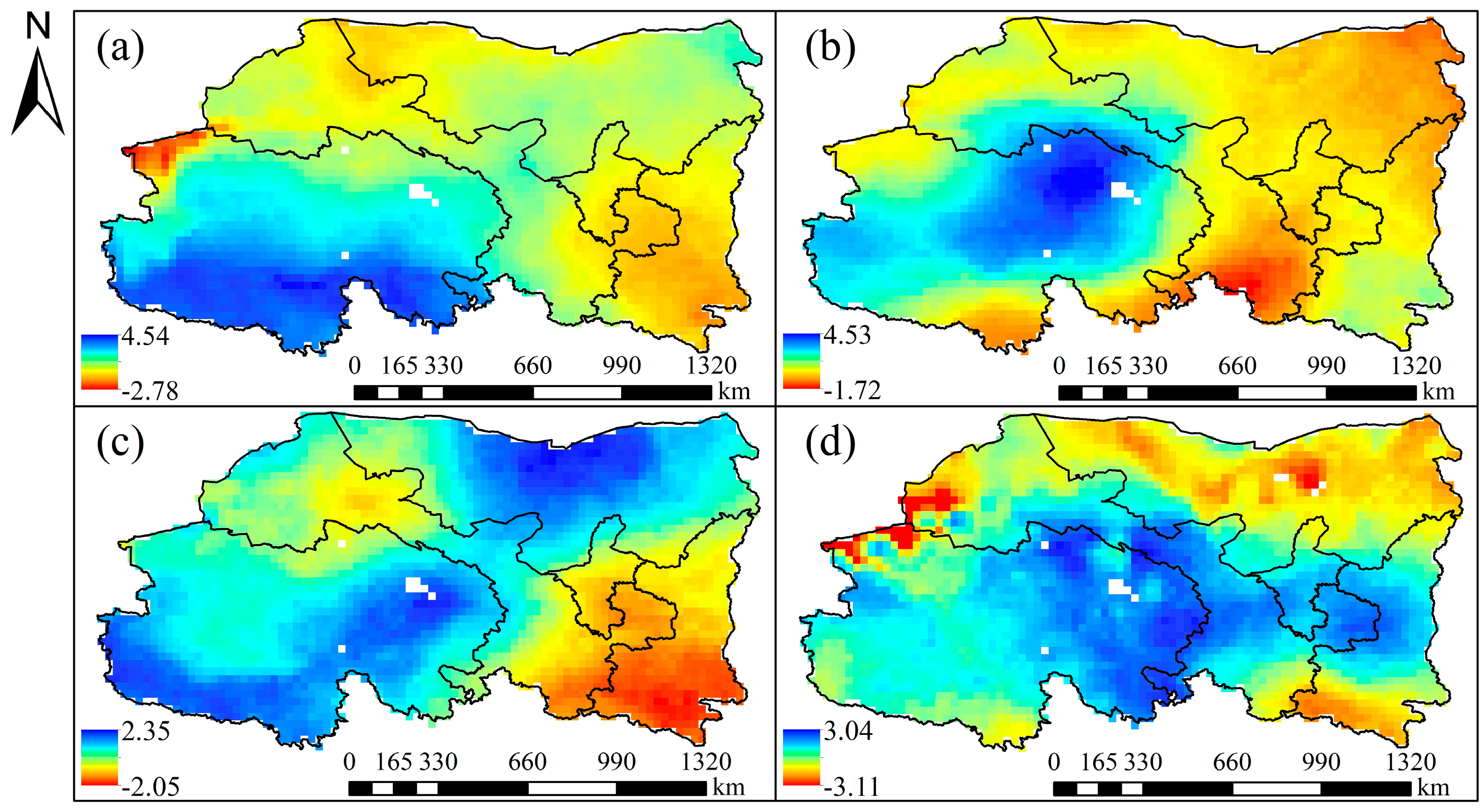
The spatial evolution characteristics of drought trends in different seasons in northwest China are shown in Figure 7. In the spring, 73.7% of the northwest region showed an upward trend in the SPEI, with a significant increase in southern Qinghai. The areas with a significant downward trend in the SPEI were mainly concentrated in the northwest of Qinghai Province, accounting for only 0.9% of the total area. In the summer, the areas with a significant upward trend in the SPEI accounted for 28.6% of the total area, mainly concentrated in Qinghai Province. However, the drought in eastern Inner Mongolia, northern Shaanxi, southern Gansu, and part of southern Qinghai showed an increasing trend, especially in southern Gansu. In the autumn, the areas with a humidification trend accounted for 71.1% of the total area, mainly concentrated in Qinghai, Inner Mongolia, and some parts of Gansu. The areas with a significant descending trend in the SPEI were concentrated in southern Shaanxi, accounting for 3.7% of the total. In the winter, the areas with an upward trend in the SPEI expanded, accounting for 83.2% of the total, and the areas with a significant humidification trend also increased. The area with a significant trend of drought accounted for only 0.8%.
In summary, the trend of droughts in different seasons in northwest China was mainly downward in the west and upward in the east, indicating a humidification trend in arid areas, while there was an aridification trend in semi-arid and semi-humid areas. From spring to winter, the humidification trend was expanding towards the east, and the areas with a significant humidification trend gradually shifted towards the east. These results indicate that the spatial distribution of droughts in northwest China tends to be uniform in the long run.

3.1.3. Spatial Variation Characteristics of Drought Intensity and Frequency

Spatial Characteristics of Drought Intensity

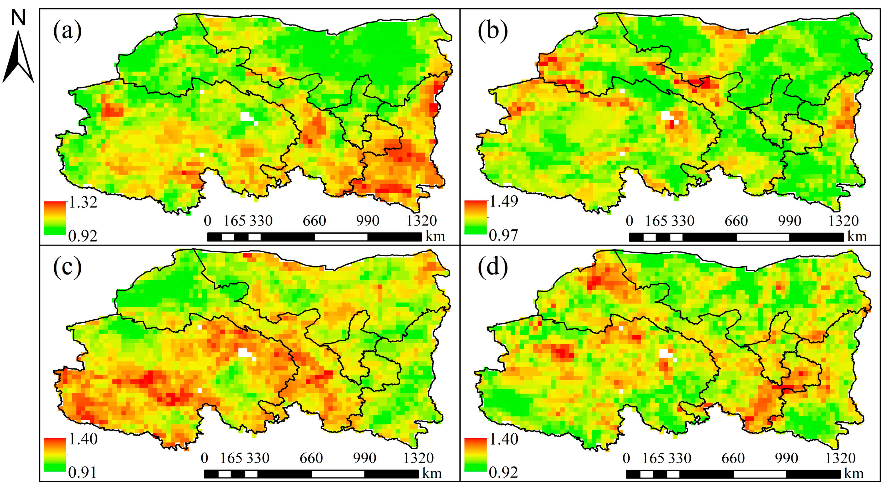
Figure 8 illustrates the spatial distribution of drought intensity in different seasons in northwest China. The high drought intensity areas in spring, covering 7.5% of the total area, were mostly found in southeastern Gansu, northwestern Qinghai, and some areas in Shaanxi, while the low drought intensity areas included central Inner Mongolia and western Gansu, accounting for 6.6% of the total area. The high drought intensity areas in summer accounted for approximately 8.3% of the total area. They were mainly distributed in northern Shaanxi, central and western Gansu, central Inner Mongolia, and northern Qinghai. Additionally, the maximum drought intensity was 1.49. This implied a more severe level of drought as compared to the other seasons, as well as a larger area of high-intensity drought. Nevertheless, the areas with low drought intensity accounted for only 0.9%. As for autumn, the high drought intensity areas, accounting for approximately 4.1% of the total area, were mainly concentrated in southwestern and northeastern Qinghai and southeastern Gansu. A considerable portion of Shaanxi, northwestern Gansu, and northwestern Qinghai had a low level of drought intensity, which accounted for 6.6% of the total area. The minimum drought intensity recorded was 0.91. In the case of winter, the proportions of the areas with high and low drought intensity were similar and small. The high-value areas included southeastern and northwestern Gansu and northern Qinghai, accounting for approximately 4.4% of the total area. The low-value areas consisted of southwestern Qinghai, northern Inner Mongolia, and southern Shaanxi, accounting for about 4.6% of the total area.

Spatial Characteristics of Drought Frequency

Figure 9 displays the spatial distribution characteristics of drought frequency in four seasons in Northwest China. As shown in the figure, the high-frequency areas of drought during spring were mainly in central Inner Mongolia, northwestern Gansu, and southwestern and northeastern Qinghai, with the drought frequency maintained at 25% or above. In contrast, southeastern Gansu, southeastern Qinghai, and Shaanxi remained at a low level of drought frequency, accounting for 15.9% of the total area in northwest China. During summer, the maximum drought frequency was 28.4%. The high-frequency areas mainly included eastern Inner Mongolia, southern Gansu, and southern Qinghai, covering 2.4% of the total area. The low-frequency areas were in northwestern Qinghai, central and western Gansu, and northern Shaanxi, with the minimum of 12.5%. The drought frequency during autumn drought had the maximum of 31.8% among the four seasons. The high-frequency areas mainly concentrated in western Gansu, northwestern and southeastern Qinghai, and the junction of Ningxia, Inner Mongolia, and Shaanxi. In contrast, the low-frequency areas of autumn drought were mainly distributed in central and northeastern Qinghai and southeastern Gansu. During winter, the high and low-frequency areas accounted for the smallest proportion of the total area. The areas with a high frequency of winter drought included southern Qinghai and southern Shaanxi, accounting for only 4.9% of the total area in northwest China. By contrast, the low-frequency areas were mainly concentrated in southeastern Gansu and central Shaanxi, accounting for only 13.7% of the total area.
The analysis shows that the spatial distribution of drought intensity and frequency in the study area exhibited opposite characteristics in the four seasons. For example, the southeastern part of the study area experienced high drought intensity but low drought frequency in spring, while the northeastern part experienced low drought intensity but high drought frequency in summer. Similarly, the northwestern part was characterized by low drought intensity but high drought frequency in autumn, whereas the southwestern part had low drought intensity but high drought frequency in winter. This indicates that the likelihood of high-intensity meteorological drought events occurring in the same area was relatively low, and low-intensity drought events were frequent.

3.2. Dynamic Evolution of Typical Drought Event

Temporal Evolution Characteristics of Drought at Different Time Scales

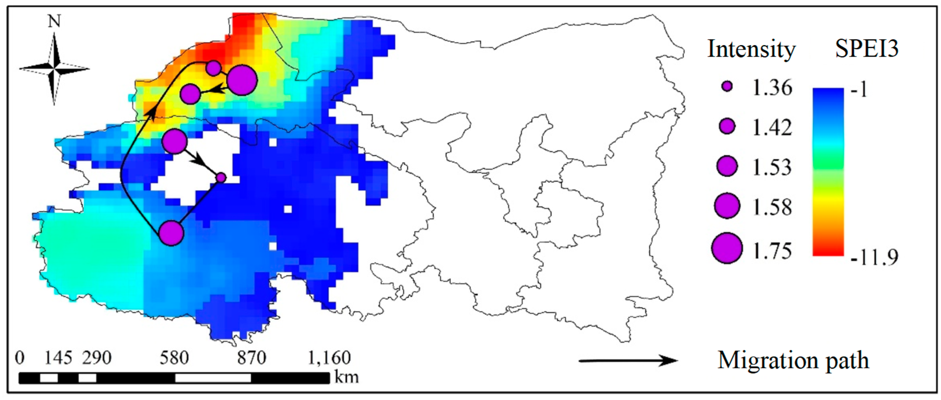
Figure 10 and Figure 11 illustrate the spatiotemporal evolution and migration path of a recent severe drought event. This drought event lasted from December 2017 to May 2018, covering a duration of 6 months. It had a severity of 2.73 × 10⁶ month·km2. The drought event initially struck an approximate area of 0.31 × 10⁶ km2, accounting for 18.10% of the total study area. The drought center was situated in the northwest part of Haixi Mongolian-Tibetan Autonomous Prefecture, Qinghai. In January 2018, the drought area rapidly expanded to 0.63 × 10⁶ km2, accounting for 35.90% of the total area. The drought center shifted southeastwards to the central part of Haixi Mongolian-Tibetan Autonomous Prefecture with a migration distance of 191.73 km. In February of the same year, the drought area and severity declined to 0.34 × 10⁶ km2 and 0.54 × 10⁶ month·km2, respectively. The drought center migrated southwestwards to the northern part of the Yushu Tibetan Autonomous Prefecture at an average velocity of 255.36 km·month−1. In March, the drought magnitude continued to weaken, and the drought area reached its minimum of 0.12 × 10⁶ km2, accounting for only 6.90% of the total study area. It was primarily concentrated in the western part of Jiuquan City, Gansu. Subsequently, the drought magnitude showed an upward trend, with an area of 0.26 × 10⁶ km2 and an intensity of 1.75, signifying the most severe level. It expanded further into central Gansu and the western part of Alxa League. In May, the drought area reduced to 0.15 × 10⁶ km2, indicating a weakened drought situation and the termination of the drought. In summary, this drought event was mainly concentrated in the western part of the study area. The migration path of the drought center was characterized by a north-south oscillation pattern, and the drought had generally experienced five processes: occurrence, aggravation, mitigation, re-aggravation, and termination.

3.3. Multivariable Frequency Analysis of Drought

3.3.1. Correlation Analysis of Drought Variables

The correlation analysis of the various combination features is the foundation for selecting Copula functions and estimating parameters. In this paper, drought events with a duration of two months or longer (a total of 160 events) were selected for multi-feature frequency analysis. Figure 12 and Table 5, respectively, show the scatter diagram and significance test results of the correlations among drought duration, intensity, and area in the study area from 1960 to 2018. It can be observed that there was a strong linear relationship (R2 > 0.6) among the drought feature variables. Moreover, each set of drought variables had high mutual dependence and a strong correlation, with a statistically significant p-value of 0.01. Therefore, it is reasonable to use the Copula function for joint distribution modeling for the frequency analysis.
As shown in Figure 12, the scatter plots of the correlation between drought duration-intensity and drought duration-area exhibit noticeable bands distributed along the vertical axis for each corresponding scale of the abscissa. This is attributed to the monthly SPEI used for drought identification, resulting in the drought duration being integer months and further a much smaller actual sample size. For example, the drought durations in the figure are only present in 2–11 months, which totals to only 10 sample values. This can affect the fitting goodness test results and parameter estimation. Furthermore, according to the Sklar theorem, the marginal distributions used for the Copula frequency analysis must be continuous functions. To achieve this, the randomization scheme proposed by De Michele et al. was adopted to transform the discrete drought duration sequence into a continuous one. This randomization method does not alter the probability distribution characteristics of the original sequence.

3.3.2. Selection of Marginal Distributions for Drought Variables

According to the K-S and A-D goodness-of-fit test results for seven candidate distribution functions, the optimal marginal distribution type for each drought feature variable was determined, and the maximum likelihood estimation was used for parameter estimation. At a significance level of p = 0.05, if the result passed the K-S test, the distribution with the smallest A-D statistic was chosen as the optimal distribution of the drought feature variable. Otherwise, the distribution was rejected directly. Table 6 lists the goodness-of-fit test results and optimal distribution parameters for each distribution function of the drought feature variables, with the optimal distribution in bold black font. It can be seen that the GP distribution is the optimal marginal distribution function for the drought duration and area, while the LogN distribution is optimal for the drought intensity. Figure 13 shows the fitting effect of the empirical frequency and theoretical frequency of the optimal marginal distribution function for drought feature variables. The data points are concentrated around the 1:1 line, indicating that the theoretical and empirical probabilities of the best-fit distribution function for drought feature variables have a good correspondence.

3.3.3. Selection of Optimal Copula Functions

According to the goodness-of-fit test results, one optimal Copula function was determined for each combination of drought feature variables from six candidate Copula functions (Gumbel, Clayton, Frank, Joe, Normal, and t) to construct the joint distribution. Table 7 lists the goodness-of-fit test results and the parameters of the optimal Copula functions. Smaller AIC, BIC, and RMSE values indicate better fitting results. The optimal Copula function is in bold black font. As shown in the table, the Frank Copula function has the smallest AIC, BIC, and RMSE values for the duration-intensity combination, making it the optimal joint model for this combination. The Gumbel Copula function performed the best in constructing the joint probability distribution of the duration-area combination, while the optimal model for the intensity-area combination was the Clayton Copula function. The optimal joint probability distribution model for the duration-intensity-area combination was constructed using the Gumbel Copula function.
Figure 14 shows the PP (probability-probability) of the theoretical cumulative probability of the optimal Copula function and the empirical Copula cumulative probability for each combination of drought feature variables. The data points of the empirical and theoretical cumulative probabilities of the joint distribution of each group of drought feature variables are evenly distributed on both sides of the diagonal line, indicating that the results of the two are roughly equal. The optimal joint distribution function can better describe the joint probability distribution between drought feature variables.

3.3.4. Joint Occurrence Probability of Drought

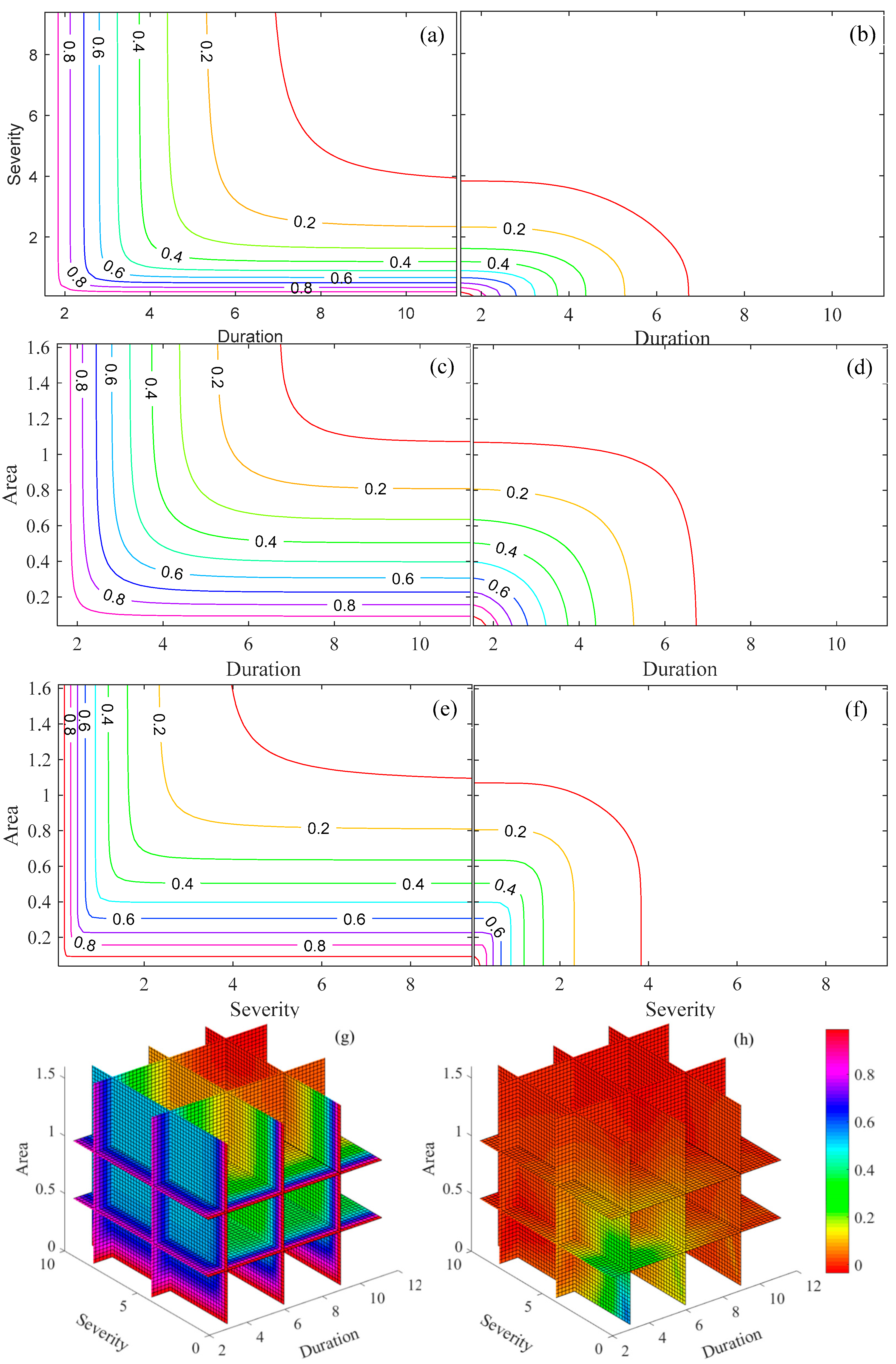
The joint occurrence probabilities between drought variables can be divided into two situations. One is when a variable, such as drought duration, severity, or area, is greater than or equal to a specific value (referred to as the “or” situation), such as P (D ≥ 5 ∪ S ≥ 2) and P (D ≥ 5 ∪ S ≥ 2 ∪ A ≥ 1). The other is when all the three drought variables simultaneously exceed a specific value (referred to as the “and” situation), such as P (D ≥ 5 ∩ S ≥ 2) and P (D ≥ 5 ∩ S ≥ 2 ∩ A ≥ 1). The bivariate and trivariate joint occurrence probabilities of drought variables are shown in Figure 15. It can be seen that the range of high joint occurrence probability in the “or” situation is much larger than that in the “and” situation. The joint occurrence probability of the same combination of drought variables is higher in the “or” situation. For example, when the drought duration and severity are greater than or equal to 4.09 months and 11.02 × 10⁶ month·km2, respectively, the joint occurrence probability in the “or” situation is 49.4%, while it is 30.2% in the “and” situation. In both situations, the joint occurrence probability increases as the drought variables decrease. For example, when the drought duration and severity exceed 6.65 months and 2.73 × 10⁶ month·km2, respectively, in the “or” situation, the joint occurrence probability is 20.1%; when they exceed 3.30 months and 1.97 × 10⁶ month·km2, respectively, the probability is 49.8%.

3.3.5. Conditional Probability of Drought

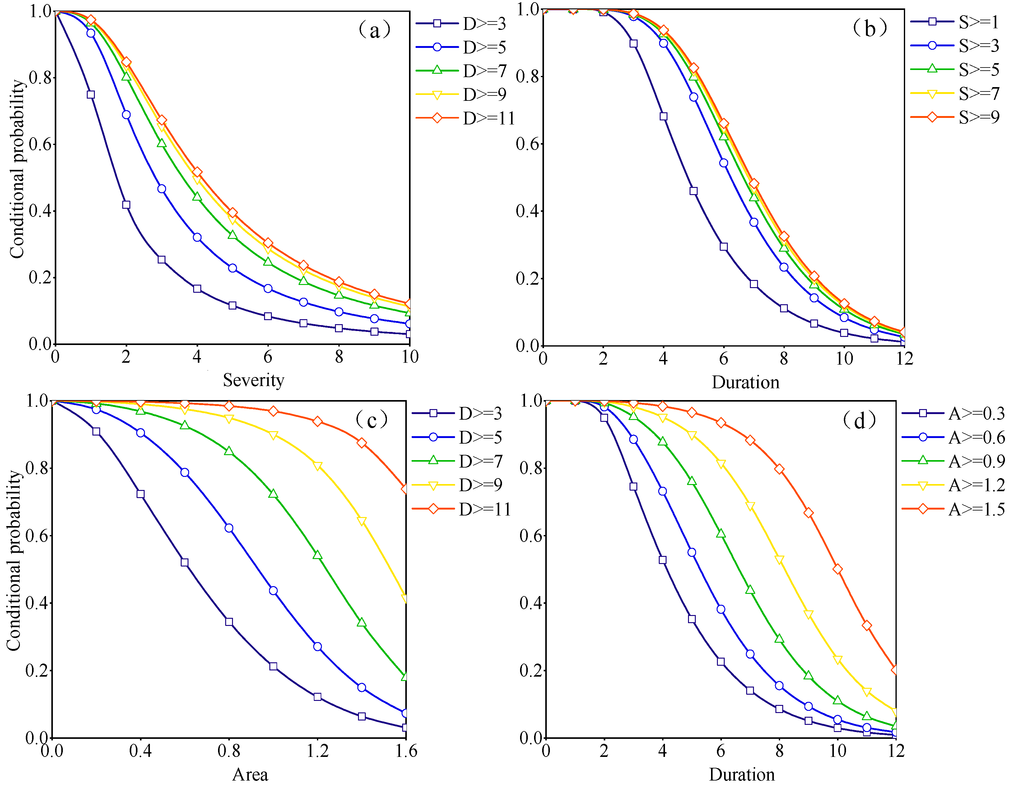
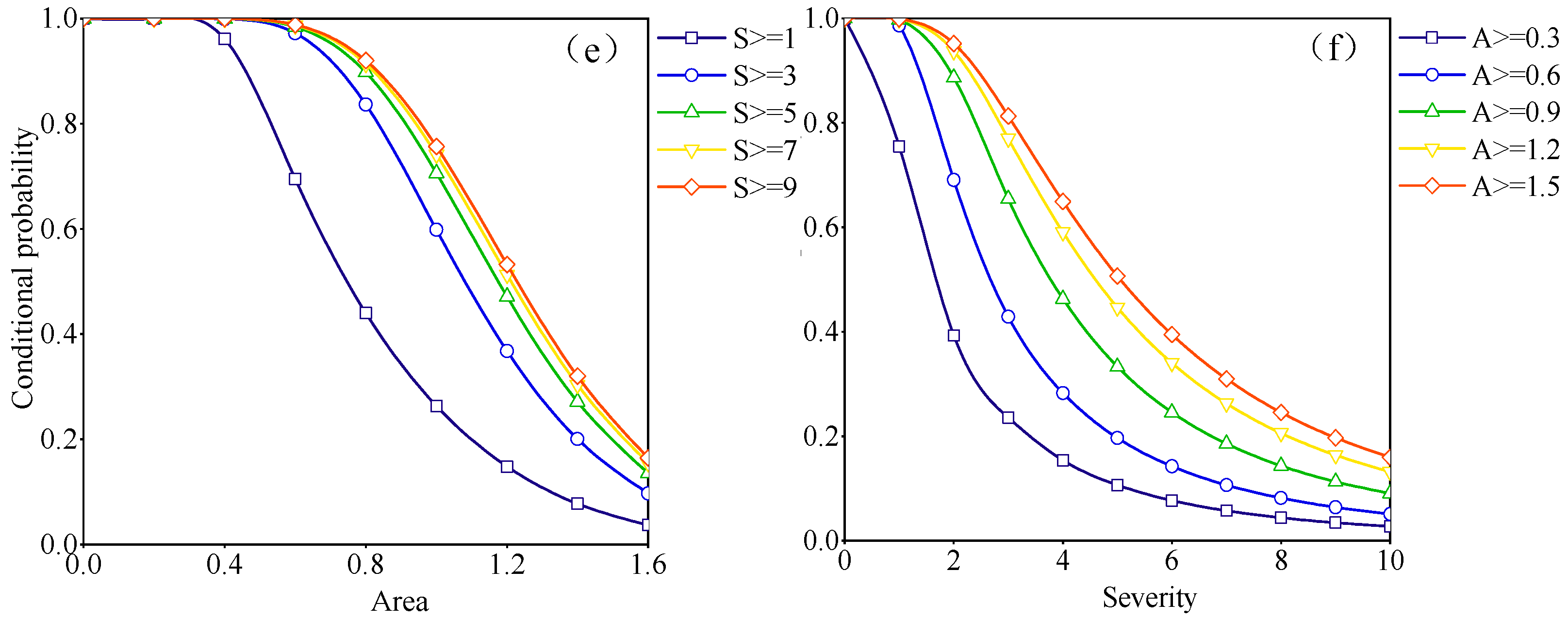
The conditional probabilities of meteorological droughts can be easily obtained based on the joint probabilities of droughts calculated using the Copula function. Figure 16 presents the two-dimensional conditional probability among drought duration, severity, and area. Figure 16a shows the conditional probability of drought severity when the drought duration exceeds a certain threshold. Figure 16b shows the conditional probability of drought duration when the drought intensity is larger than a certain threshold. The results indicate that with increasing conditional factors, both the conditional probabilities of drought severity and duration show a rising trend. Specific probabilities can be determined for a given conditional factor from the figure. For instance, given a drought duration of more than 5 months and drought severity of more than 1 × 10⁶ month·km2, the probability of drought is 93.4%. It means that there is a high likelihood of meteorological drought under such conditions. Furthermore, if the drought severity is larger than 1, 3, 5, 7, or 9 × 10⁶ month·km2 and the drought duration is greater than 5 months, the probability of meteorological drought will be 46.2%, 73.9%, 79.8%, 81.7%, and 82.6%, respectively. The distribution characteristics of probability show a dense distribution at both ends and a sparse distribution in the middle, indicating the difference in probability results at different conditional factor levels. For example, when the drought severity is high (Figure 16a), the probability results for different conditional factors have little difference. Additionally, an increase in the conditional factor (drought duration) will significantly raise the probability of meteorological drought events with moderate intensity, similar to the results of Yusof et al. [45].
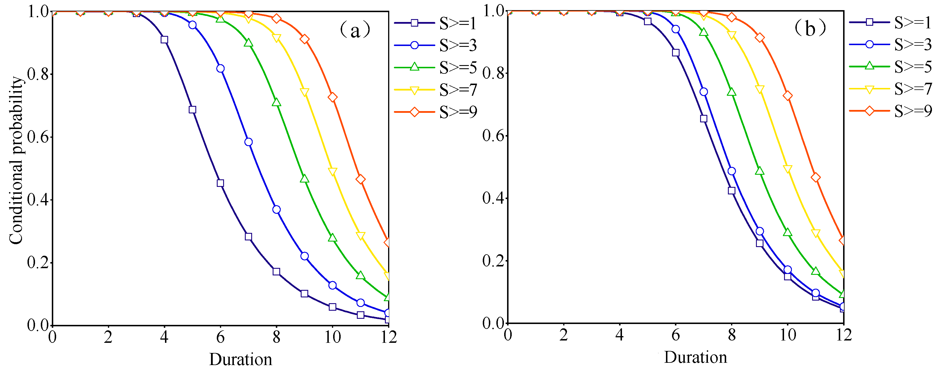
Figure 17 presents the conditional probability of meteorological drought for three drought variable combinations. As shown in Figure 16 and Figure 17, the conditional probability of meteorological drought under three drought variables is greater than that under two. For example, in the case of a drought severity above 5 × 10⁶ month·km2 and a drought duration longer than 5 months, the conditional probability of meteorological drought is 79.8%. Meanwhile, given a drought area greater than 1 × 10⁶ km2, this figure increases to 99.8%. It can be concluded that ignoring any drought variable may significantly underestimate the occurrence probability of severe meteorological droughts, as well as the severity of drought events [17].

4. Discussion

This study found that the temporal variation in the drought index represented an ascending trend in Northwestern China due to a continuous increase in precipitation and temperature [46].Especially, this phenomenon was significant in arid regions, which indicates that runoff and glacier ablation continued to increase, and the water level of inland lakes increased significantly, the rise and flood disasters increased, while the vegetation improved and the number of sandstorm days decreased [47,48]. Moreover, the warm-wet tendency in northwest China exhibits an obvious response to the “global warming stagnation” [49].
The present climate in northwest China has been changing from warm-dry to warm-wet [50], and the 1980s was the turning point of drought. Taking the annual scale drought index series as an example, the moving T test is used to detect the change point of drought in the study area. The step is set to 6, for a fixed significance level of p = 0.05 in the present paper, and the corresponding critical value is 2.31 (Figure 18). Obviously, the statistical value exceeded the reliable lines of the significance level (p = 0.05) between 1981 and 1985. Therefore, the change points of the annual drought index were concentrated between 1981 and 1985, and the property (positive or negative) of the maximum change point (in 1993) could be used to estimate the main trend of the drought index series.
Similar studies have pointed out the late 1980s were the abrupt wetting point of drought. For example, Wang et al. [51] found that there were two evident contrasting periods of drought between 1961 and 2010. Sustaining drought conditions existed between 1961 and 1986, whereas wet conditions dominated after 1986. Li et al. [52] reported a weakening drought in Northwestern China based on the increasing trends of the SPI series. Additionally, as the variation of annual precipitation in northwest China showed a significant upward trend in the central and west of the study region, and a downward trend in the eastern regions [53,54], the SPEI exhibited a fluctuating upward trend in the plateau climate zone and westerly climate zone, while there was a trend towards aridity in the southeast climate zone.
In summary, joint occurrence probabilities can quantitatively capture the occurrence probability of meteorological drought under different drought variables, providing important information for drought mitigation and water resource management. For example, the occurrence probability of meteorological drought with a certain duration and intensity can serve as a critical condition for identifying specific water supply systems and triggering drought emergency plans [55]. Overestimation of drought risk may occur if only the “or” situation is considered, while underestimation may occur if only the “and” situation is considered. Therefore, a comprehensive analysis of both situations is necessary to ensure an accurate assessment of the occurrence probability of meteorological drought. Additionally, the conditional occurrence probability is useful for assessing water resource systems under extreme drought conditions and determining if the systems can meet the water demand under given drought conditions. This information allows water resource managers to quickly determine the amount of additional water needed to alleviate drought.

5. Conclusions

In this study, the SPEI calculated based on the gridded data from 1960 to 2018 was used to estimate meteorological drought. Drought events were identified through a 3D identification method, showing the dynamic evolution of drought events. The optimal marginal distribution of drought variables was selected from seven alternative distributions. Moreover, the best-fitted Copula was selected from six candidate Copulas using the RMSE, AIC, and BIC methods. These selected Copulas were employed to estimate drought risk through bivariate and trivariate joint probability and conditional probability analyses, respectively. The major conclusions are as follows:
(1)
Overall, the SPEI showed an upward trend in the plateau climate zone and the westerly climate zone, with rates of 0.188/10a and 0.046/10a, indicating a mitigation of drought. Conversely, the SPEI demonstrated a descending trend (−0.038/10a) in the southeast climate zone, suggesting an intensified drought situation.
(2)
The variation trend of drought in different seasons was mainly downward in the west part and upward in the east part of Northwestern China. From spring to winter, the humidification trend expanded towards the east, and the areas with a significant humidification trend gradually shifted towards the east.
(3)
The spatial distribution of drought intensity and frequency in different seasons exhibited opposite characteristics. For example, the southeastern part of the study area experienced a high drought intensity but a low drought frequency in spring. This indicated that the likelihood of high-intensity meteorological drought events occurring in the same area was relatively low, whereas low-intensity drought events were frequent.
(4)
The most severe drought event occurred from January 1961 to October 1962 and experienced five processes: occurrence, aggravation, mitigation, re-aggravation, and termination. The migration path was characterized by north-south oscillation.
(5)
The joint occurrence probabilities were consistently higher in the “or” situation than in the “and” situation for the same combination of drought variables. Furthermore, the conditional probability of drought variables, given specific conditional factors, declined as the values of these factors increased. Notably, as the conditional factors increased, there was a noticeable reduction in the drought occurrence probability for drought variables with lower values.

Author Contributions

Conceptualization, K.F. and Y.W.; data interpretation and methodology, F.W. and W.Z.; validation, W.W.; software, Z.Z., original draft preparation, K.F.; funding acquisition, W.Z.; K.F., F.W. and S.H. All authors have read and agreed to the published version of the manuscript.

Funding

This research was supported by Yinshanbeilu Grassland Eco-hydrology National Observation and Research Station, China Institute of Water Resources and Hydropower Research (grant number YSS202112, YSS202101 and YSS202118), Special Research Project of China Institute of Water Resources and Hydropower Research (MK2022J07), Key Special Project of the “Science and Technology Revitalization of Mongolia” Action (grant number 2022EEDSKJXM004-4), National Natural Science Fund of China (grant number 42301024, 52079111 and 52179015), Science and Technology Projects in Henan Province (grant number 222102320043 and 201300311400), and State Key Laboratory of Simulation and Regulation of Water Cycle in River Basin (grant number IWHR-SKL-KF202212).

Data Availability Statement

Data available on request from the authors. The data that support the findings of this study are available from the corresponding author upon reasonable request.

Conflicts of Interest

The authors declare no conflict of interest.

References

  1. Vicente-Serrano, S.; Beguería, S.; López-Moreno, J.I. A Multi-scalar Drought Index Sensitive to Global Warming: The Standardized Precipitation Evapotranspiration Index. J. Clim. 2010, 23, 1696–1718. [Google Scholar] [CrossRef]
  2. Tong, S.; Lai, Q.; Zhang, J.; Bao, Y.; Lusi, A.; Ma, Q.; Li, X.; Zhang, F. Spatiotemporal drought variability on the Mongolian Plateau from 1980–2014 based on the SPEI-PM, intensity analysis and Hurst exponent. Sci. Total Environ. 2018, 615, 1557–1565. [Google Scholar] [CrossRef] [PubMed]
  3. Sun, S.; Li, Q.; Li, J.; Wang, G.; Zhou, S.; Chai, R.; Hua, W.; Deng, P.; Wang, J.; Lou, W. Revisiting the evolution of the 2009–2011 meteorological drought over Southwest China. J. Hydrol. 2019, 568, 385–402. [Google Scholar] [CrossRef]
  4. Yoo, J.; Kim, J.; Kwon, H.; Kim, T. A new drought monitoring approach using three-dimensional drought properties based on a dynamic drought detection technique algorithm. J. Hydrol. Reg. Stud. 2022, 44, 101270. [Google Scholar] [CrossRef]
  5. Gocic, M.; Trajkovic, S. Spatiotemporal characteristics of drought in Serbia. J. Hydrol. 2014, 510, 110–123. [Google Scholar] [CrossRef]
  6. Chen, Z.; Yang, G. Analysis of drought hazards in North China: Distribution and interpretation. Nat. Hazards 2013, 65, 279–294. [Google Scholar] [CrossRef]
  7. He, B.; Chang, J.; Wang, Y.; Wang, Y.; Zhou, S.; Chen, C. Spatio-temporal evolution and non-stationary characteristics of meteorological drought in inland arid areas. Ecol. Indic. 2021, 126, 107644. [Google Scholar] [CrossRef]
  8. Zhou, H.; Liu, Y.; Liu, Y. An Approach to Tracking Meteorological Drought Migration. Water Resour. Res. 2019, 55, 3266–3284. [Google Scholar] [CrossRef]
  9. Wen, X.; Tu, Y.; Tan, Q.; Li, W.; Fang, G.; Ding, Z.; Wang, Z. Construction of 3D drought structures of meteorological drought events and their spatio-temporal evolution characteristics. J. Hydrol. 2020, 590, 125539. [Google Scholar] [CrossRef]
  10. Lloyd-Hughes, B.A. spatio-temporal structure-based approach to drought characterisation. Int. J. Climatol. 2012, 32, 406–418. [Google Scholar] [CrossRef]
  11. Tosunoglu, F.; Can, I. Application of copulas for regional bivariate frequency analysis of meteorological droughts in Turkey. Nat. Hazards 2016, 82, 1457–1477. [Google Scholar] [CrossRef]
  12. Salvadori, G.; De Michele, C. Multivariate real-time assessment of droughts via copula-based multi-site Hazard Trajectories and Fans. J. Hydrol. 2015, 526, 101–115. [Google Scholar] [CrossRef]
  13. Lee, T.; Modarres, R.; Ouarda, T.B.M.J. Data-based analysis of bivariate copula tail dependence for drought duration and severity. Hydrol. Process. 2013, 27, 1454–1463. [Google Scholar] [CrossRef]
  14. Huang, S.; Hou, B.; Chang, J.; Huang, Q.; Chen, Y. Copulas-based probabilistic characterization of the combination of dry and wet conditions in the Guanzhong Plain, China. J. Hydrol. 2014, 519, 3204–3213. [Google Scholar] [CrossRef]
  15. Ma, M.; Song, S.; Ren, L.; Jiang, S.; Song, J. Multivariate drought characteristics using trivariate Gaussian and Student t copulas. Hydrol. Process. 2013, 27, 1175–1190. [Google Scholar] [CrossRef]
  16. Ma, M.; Zang, H.; Wang, W.; Cui, H.; Sun, Y.; Cheng, Y. Copula-Based Severity-Duration-Frequency (SDF) Analysis of Streamflow Drought in the Source Area of the Yellow River, China. Water 2023, 15, 2741. [Google Scholar] [CrossRef]
  17. Xu, K.; Yang, D.; Xu, X.; Lei, H. Copula based drought frequency analysis considering the spatio-temporal variability in Southwest China. J. Hydrol. 2015, 527, 630–640. [Google Scholar] [CrossRef]
  18. Hua, L.; Zhong, L.; Ma, Z. Decadal transition of moisture sources and transport in northwestern China during summer from 1982 to 2010. J. Geophys. Res. Atmos. 2017, 122, 12522–12540. [Google Scholar] [CrossRef]
  19. Zhang, Q.; Yang, J.; Wang, W.; Ma, P.; Lu, G.; Liu, X.; Yu, H.; Fang, F. Climatic warming and humidification in the arid region of Northwest China: Multi-scale characteristics and impacts on ecological vegetation. J. Meteorol. Res. 2021, 35, 113–127. [Google Scholar] [CrossRef]
  20. Liu, C.; Huang, W.; Feng, S.; Chen, J.; Zhou, A. Spatiotemporal variations of aridity in China during 1961–2015: Decomposition and attribution. Sci. Bull. 2018, 63, 1187–1199. [Google Scholar] [CrossRef]
  21. Park, C.E.; Jeong, S.J.; Ho, C.H.; Park, H.; Piao, S.; Kim, J.; Feng, S. Dominance of climate warming effects on recent drying trends over wet monsoon regions. Atmos. Chem. Phys. 2017, 17, 10467–10476. [Google Scholar] [CrossRef]
  22. Zhong, L.; Hua, L.; Yao, Y.; Feng, J. Interdecadal aridity variations in Central Asia during 1950–2016 regulated by oceanic conditions under the background of global warming. Clim. Dyn. 2021, 56, 3665–3686. [Google Scholar] [CrossRef]
  23. Jiang, T.; Su, X.; Singh, V.P.; Zhang, G. Spatio-temporal pattern of ecological droughts and their impacts on health of vegetation in Northwestern China. J. Environ. Manag. 2022, 305, 114356. [Google Scholar] [CrossRef] [PubMed]
  24. Han, Z.; Zhang, B.; Yang, L.; He, C. Assessment of the impact of future climate change on maize yield and water use efficiency in agro-pastoral ecotone of Northwestern China. J. Agron. Crop Sci. 2021, 207, 317–331. [Google Scholar] [CrossRef]
  25. Cao, S.; He, Y.; Zhang, L.; Chen, Y.; Yang, W.; Yao, S.; Sun, Q. Spatiotemporal characteristics of drought and its impact on vegetation in the vegetation region of Northwest China. Ecol. Indic. 2021, 133, 108420. [Google Scholar] [CrossRef]
  26. Zhang, G.; Su, X.; Ayantobo, O.O.; Feng, K.; Guo, J. Remote-sensing precipitation and temperature evaluation using soil and water assessment tool with multi-objective calibration in the Shiyang River Basin, Northwest China. J. Hydrol. 2020, 590, 125416. [Google Scholar] [CrossRef]
  27. Feng, K.; Li, Y.; Wang, F.; Su, X.; Wu, H. Analysis of drought events in Northwest China based on an improved three-dimensional identification method. Water Resour. Prot. 2023, 39, 63–72. [Google Scholar]
  28. Yang, M.; Yan, D.; Yu, Y.; Yang, Z.; Gonzalez, J.E. SPEI-Based Spatiotemporal Analysis of Drought in Haihe River Basin from 1961 to 2010. Adv. Meteorol. 2016, 2016, 7658015. [Google Scholar] [CrossRef]
  29. Wang, Y.; Wang, Z.; Zhang, Z.; Shen, D.; Zhang, L. The best-fitting distribution of water balance and the spatiotemporal characteristics of drought in Guizhou Province, China. Theor. Appl. Climatol. 2021, 143, 1097–1112. [Google Scholar] [CrossRef]
  30. Mathbout, S.; Lopez-Bustins, J.A.; Martin-Vide, J.; Bech, J.; Rodrigo, F.S. Spatial and temporal analysis of drought variability at several time scales in Syria during 1961–2012. Atmos. Res. 2018, 200, 153–168. [Google Scholar] [CrossRef]
  31. Wable, P.; Jha, M.; Shekhar, A. Comparison of Drought Indices in a Semi-Arid River Basin of India. Water Resour. Manag. 2019, 33, 75–102. [Google Scholar] [CrossRef]
  32. Wang, F.; Wang, Z.; Yang, H.; Di, D.; Zhao, Y.; Liang, Q. Utilizing GRACE-based groundwater drought index for drought characterization and teleconnection factors analysis in the North China Plain. J. Hydrol. 2020, 585, 124849. [Google Scholar] [CrossRef]
  33. Guo, Y.; Huang, S.; Huang, Q.; Wang, H.; Fang, W.; Yang, Y.; Wang, L. Assessing socioeconomic drought based on an improved Multivariate Standardized Reliability and Resilience Index. J. Hydrol. 2019, 568, 904–918. [Google Scholar] [CrossRef]
  34. Wang, F.; Yang, H.; Wang, Z.; Zhang, Z.; Li, Z. Drought Evaluation with CMORPH Satellite Precipitation Data in the Yellow River Basin by Using Gridded Standardized Precipitation Evapotranspiration Index. Remote Sens. 2019, 11, 485. [Google Scholar] [CrossRef]
  35. Araujo, M.V.O.; Celeste, A.B. Rescaled range analysis of streamflow records in the São Francisco River Basin, Brazil. Theor. Appl. Climatol. 2019, 135, 249–260. [Google Scholar] [CrossRef]
  36. Zhang, D.; Ge, W.; Zhang, Y. Evaluating the vegetation restoration sustainability of ecological projects: A case study of Wuqi County in China. J. Clean. Prod. 2020, 264, 121751. [Google Scholar] [CrossRef]
  37. Li, J.; Wu, C.; Xia, C.; Yeh, P.J.-F.; Chen, B.; Lv, W.; Hu, B.X. A voxel-based three-dimensional framework for flash drought identification in space and time. J. Hydrol. 2022, 608, 127568. [Google Scholar] [CrossRef]
  38. Diaz, V.; Corzo Perez, G.A.; Van Lanen, H.A.J.; Solomatine, D.; Varouchakis, E.A. An approach to characterizing spatio-temporal drought dynamics. Adv. Water Resour. 2020, 137, 103512. [Google Scholar] [CrossRef]
  39. Ayantobo, O.O.; Wei, J.; Wang, G. Modeling Joint Relationship and Design Scenarios Between Precipitation, Surface Temperature, and Atmospheric Precipitable Water Over Mainland China. Earth Space Sci. 2021, 8, e1513E–e2020E. [Google Scholar] [CrossRef]
  40. Xiao, M.; Yu, Z.; Zhu, Y. Copula-based frequency analysis of drought with identified characteristics in space and time: A case study in Huai River basin, China. Theor. Appl. Climatol. 2019, 137, 2865–2875. [Google Scholar] [CrossRef]
  41. Pontes Filho, J.; Souza Filho, F.; Martins, E.; de Carvalho Studart, T. Copula-Based Multivariate Frequency Analysis of the 2012–2018 Drought in Northeast Brazil. Water 2020, 12, 834. [Google Scholar] [CrossRef]
  42. Azam, M.; Maeng, S.; Kim, H.; Murtazaev, A. Copula-based stochastic simulation for regional Drought risk assessment in South Korea. Water 2018, 10, 359. [Google Scholar] [CrossRef]
  43. Kim, J.E.; Yoo, J.; Chung, G.H.; Kim, T.-W. Hydrologic Risk Assessment of Future Extreme Drought in South Korea Using Bivariate Frequency Analysis. Water 2019, 11, 2052. [Google Scholar] [CrossRef]
  44. Zhao, L.; Li, J.; Shi, Q. The temporal and spatial characteristics of drought in northwest China are analyzed based on Z index. Agric. Henan 2016, 5, 43–60. (In Chinese) [Google Scholar]
  45. Yusof, F.; Hui-Mean, F.; Suhaila, J.; Yusof, Z. Characterisation of Drought Properties with Bivariate Copula Analysis. Water Resour. Manag. 2013, 27, 4183–4207. [Google Scholar] [CrossRef]
  46. Zhang, Q.; Yang, J.; Duan, X.; Ma, P.; Lu, G.; Zhu, B.; Yue, P.; Wang, Y.; Liu, W. The eastward expansion of the climate humidification trend in northwest China and the synergistic influences on the circulation mechanism. Clim. Dynam. 2022, 59, 2481–2497. [Google Scholar] [CrossRef]
  47. Shi, Y.; Shen, Y.; Kang, E.; Li, D.; Ding, Y.; Zhang, G.; Hu, R. Recent and future climate change in northwest China. Clim. Chang. 2007, 80, 379–393. [Google Scholar] [CrossRef]
  48. Wu, P.; Liu, Y.; Ding, Y.; Li, X.; Wang, J. Modulation of sea surface temperature over the North Atlantic and Indian-Pacific warm pool on interdecadal change of summer precipitation over northwest China. Int. J. Clim. 2022, 42, 8526–8538. [Google Scholar] [CrossRef]
  49. Feng, K.P.; Tian, J.C.; Shen, H. Temperature variation characteristics of Northwest China based on K-means clustering partition in the past half century. Arid Land Geogr. 2019, 42, 1239–1252. (In Chinese) [Google Scholar]
  50. Zhang, Q.; Lin, J.; Liu, W.; Han, L. Precipitation seesaw phenomenon and its formation mechanism in the eastern and western parts of Northwest China during the flood season. Sci. China Earth Sci. 2019, 62, 2083–2098. [Google Scholar] [CrossRef]
  51. Wang, Z.; Li, J.; Lai, C.; Zeng, Z.; Zhong, R.; Chen, X.; Zhou, X.; Wang, M. Does drought in China show a significant decreasing trend from 1961 to 2009? Sci. Total Environ. 2017, 579, 314–324. [Google Scholar] [CrossRef] [PubMed]
  52. Li, H.; Hou, E.; Deng, J. Spatio-Temporal Differentiation Characteristic and Evolution Process of Meteorological Drought in Northwest China from 1960 to 2018. Front. Earth Sci. 2022, 10, 857953. [Google Scholar] [CrossRef]
  53. Wei, K.; Wang, L. Reexamination of the Aridity Conditions in Arid Northwestern China for the Last Decade. J. Clim. 2013, 26, 9594–9602. [Google Scholar] [CrossRef]
  54. Wen, X.; Wu, X.; Gao, M. Spatiotemporal variability of temperature and precipitation in Gansu Province (Northwest China) during 1951–2015. Atmos. Res. 2017, 197, 132–149. [Google Scholar] [CrossRef]
  55. Shiau, J. Fitting Drought Duration and Severity with Two-Dimensional Copulas. Water Resour. Manag. 2006, 20, 795–815. [Google Scholar] [CrossRef]
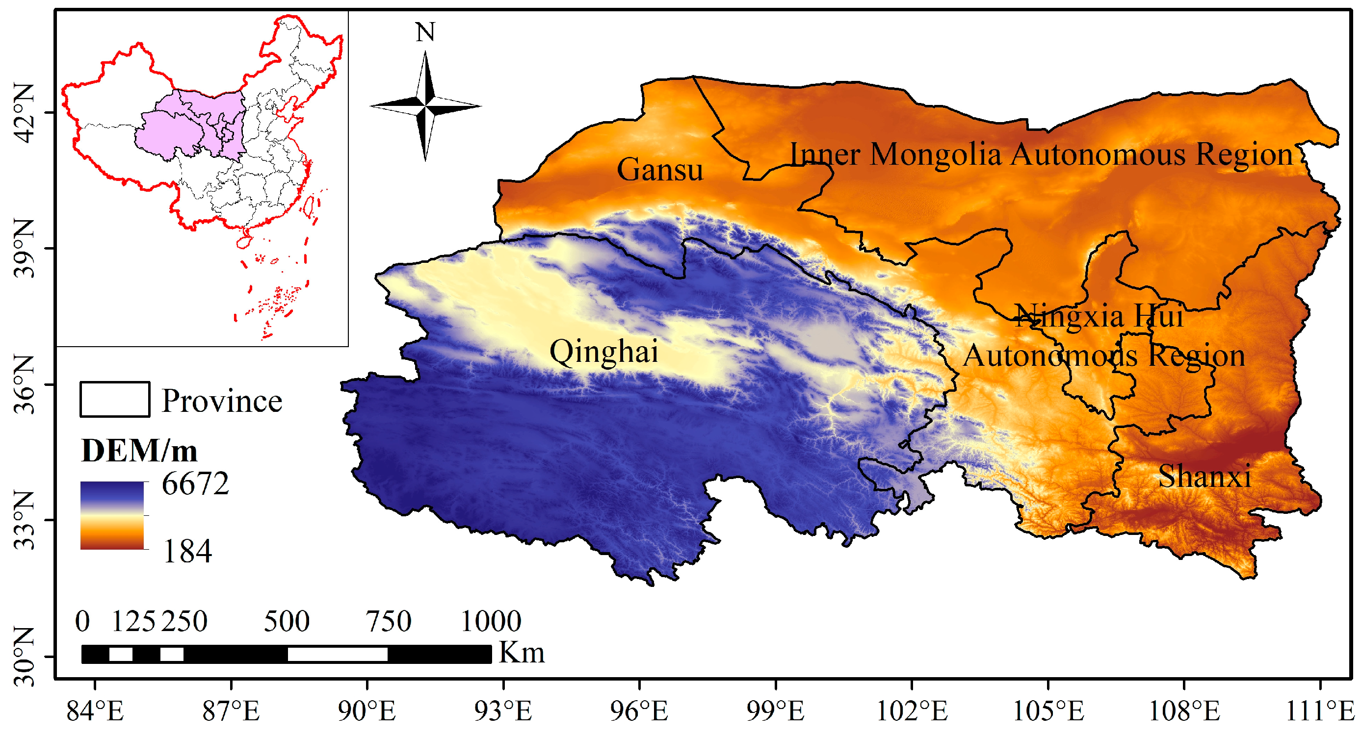
Figure 1. Location and topography of Northwestern China.
Water 15 03861 g001
Figure 2. Schematic diagrams of (a) spatial identification and (b) temporal connection of drought patches.
Water 15 03861 g002
Figure 3. Temporal evolution characteristics of SPEI series at different timescales. (a) Northwest region (b) Plateau climate zone (c) Westerlies climate zone (d) Southeast climate zone.
Water 15 03861 g003
Figure 4. Temporal evolution characteristics of SPEI series at different timescales in northwestern regions between 1960 and 2018: (a) northwestern China; (b) Pplateau climate zone; (c) westerlies climate zone; (d) southeast climate zone.
Water 15 03861 g004
Figure 5. Temporal change characteristics of seasonal SPEI series in northwestern regions during 1960–2018: (a) spring; (b) summer; (c) autumn; (d) winter.
Water 15 03861 g005
Figure 6. Variation trend of monthly SPEI series in northwestern regions between 1960 and 2018 (“*” and “**” denote significant at 0.1 and 0.05 levels, respectively).
Water 15 03861 g006
Figure 7. Spatial distributions of change trend of seasonal SPEI series in northwestern regions between 1960 and 2018: (a) spring; (b) summer; (c) autumn; (d) winter.
Water 15 03861 g007
Figure 8. Spatial distributions of seasonal drought intensity in northwestern regions between 1960 and 2018: (a) spring; (b) summer; (c) autumn; (d) winter.
Water 15 03861 g008
Figure 9. Spatial distribution of seasonal drought frequency in northwestern regions between 1960 and 2018: (a) spring; (b) summer; (c) autumn; (d) winter.
Water 15 03861 g009
Figure 10. Spatiotemporal dynamic evolution of the No.338 meteorological drought (December 2017–May 2018).
Water 15 03861 g010
Figure 11. Migration path of drought center of the No.338 meteorological drought (December 2017–May 2018). Note: the color bar denotes the cumulative value of SPEI3.
Water 15 03861 g011
Figure 12. The correlation of the pairwise drought duration, severity, and affected area.
Water 15 03861 g012
Figure 13. Probability-probability (PP) plot of meteorological drought duration, severity, and area.
Water 15 03861 g013
Figure 14. Probability-probability (PP) plot of the optimal Copula function: (a) duration-severity; (b) duration-area; (c) severity-area; (d) duration-severity-area.
Water 15 03861 g014
Figure 15. The bivariate and trivariate joint occurrence probability of drought duration (month), severity (106 month·km2), and area (106 km2): (a,c,e,g) indicate “or” situation; (b,d,f,h) indicate “and” situation.
Water 15 03861 g015
Figure 16. The conditional probability of (a) severity (106 month·km2) given that duration exceeds a certain value, (b) duration (month) given that severity exceeds a certain value, (c) area (106 km2) given that duration exceeds a certain value, (d) duration (month) given that area exceeds a certain value, (e) area (106 km2) given that severity exceeds a certain value, and (f) severity (106 month·km2) given that area exceeds a certain value.
Water 15 03861 g016aWater 15 03861 g016b
Figure 17. The conditional probability of duration (month) given that severity (106 month·km2) exceeds a certain value and area (106 km2) exceeds (a) 0.6 × 10⁶ km2 and (b) 1 × 10⁶ km2.
Water 15 03861 g017
Figure 18. Moving T test of drought index series between 1960 and 2018.
Water 15 03861 g018
Table 1. Drought level classification based on SPEI.
Drought LevelSPEIDrought Severity
I−0.5 < SPEINo drought
II−1.0 < SPEI ≤ −0.5Mild drought
III−1.5 < SPEI ≤ −1.0Moderate drought
IV−2.0 < SPEI ≤ −1.5Severe drought
VSPEI ≤ −2Extreme drought
Table 2. Cumulative probability distribution function and parameters.
Distribution
Types
Cumulative Probability DistributionParameters
Gam F ( x ) = Γ x / β ( α ) Γ ( α ) α: shape parameter
β: scale parameter
LogL F ( x ) = ( 1 + ( β α ) α ) 1 α: shape parameter (α > 0)
β: scale parameter (β > 0)
LogN F ( x ) = Φ ( ln x μ σ ) μ: location parameter
σ: scale parameter
Wb F ( x ) = 1 exp ( ( x β ) α ) α: shape parameter
β: scale parameter
P-III F ( x ) = 0 x μ β t α 1 exp ( t ) d t Γ ( α ) α: shape parameter
β: scale parameter
μ: location parameter
GEV F ( x ) = { exp ( ( 1 + k ( x μ σ ) 1 k ) ) ,   k 0 exp ( exp ( ( x μ σ ) ) ) ,   k = 0 k: shape parameter
σ: scale parameter (σ>0)
μ: location parameter
GP F ( x ) = { 1 ( 1 + k ( x μ ) σ ) 1 k ,   k 0 1 exp ( ( x μ ) σ ) ,   k = 0 k: shape parameter
σ: scale parameter (σ > 0)
μ: location parameter
Table 3. Function expressions of six Copula functions.
CopulaFunction ExpressionParameters
Frank C F ( u 1 , u 2 , , u d ; θ ) = 1 θ ln [ 1 + j = 1 d e θ u j 1 ( e θ 1 ) d 1 ] θ R \ 0
Clayton C C ( u 1 , u 2 , , u d ; θ ) = [ ( j = 1 d u j θ ) d + 1 ] θ [ 1 ,   ) \ 0
Gumbel C G ( u 1 , u 2 , , u d ; θ ) = exp { [ j = 1 d ( ln u j ) θ ] 1 θ } θ [ 1 ,   )
Joe C J ( u 1 , u 2 , , u d ; θ ) = 1 [ j = 1 d ( 1 u j ) θ j = 1 d ( 1 u j ) θ ] 1 θ θ [ 1 ,   )
Normal C N ( u 1 , u 2 , , u d ; ) = Φ ( Φ 1 ( u 1 ) , , Φ 1 ( u d ) ) = [ 1 ρ 1 d ρ 1 d 1 ]
Student t C t ( u 1 , u 2 , , u d ; , υ ) = T , υ ( T υ 1 ( u 1 ) , , T υ 1 ( u d ) ) = [ 1 ρ 1 d ρ 1 d 1 ]
Table 4. Past and future variation trends of seasonal SPEI series in northwestern regions.
SPEI SeriesTrend StatisticsHurst IndexPast TrendPersistence and Future Trend
Northwestern regionsSpring1.730.54Significant increasePersistence: increase
Summer1.750.52Significant increasePersistence: increase
Autumn0.900.62IncreasePersistence: increase
Winter2.090.59Significant increasePersistence: increase
Plateau climate zoneSpring2.990.63Significant increasePersistence: increase
Summer3.060.57Significant increasePersistence: increase
Autumn1.490.60IncreasePersistence: increase
Winter2.190.64Significant increasePersistence: increase
Westerlies
climate zone
Spring0.180.48IncreaseUnsustainability: decrease
Summer0.560.53IncreasePersistence: increase
Autumn0.900.56IncreasePersistence: increase
Winter0.340.49IncreaseUnsustainability: decrease
Southeast climate zoneSpring0.100.47IncreaseUnsustainability: decrease
Summer0.120.55IncreasePersistence: increase
Autumn−0.860.65DecreasePersistence: decrease
Winter1.770.53Significant increasePersistence: increase
Table 5. Pearson, Kendall, and Spearman correlation coefficients of drought variables.
Drought VariablesPearsonKendallSpearman
Duration-Severity0.83 **0.67 **0.82 **
Duration-Area0.77 **0.57 **0.72 **
Severity-Area0.93 **0.84 **0.97 **
Note: “**” indicates significant at the 0.01 level.
Table 6. The optimal marginal distributions and its parameters of drought variables.
Drought VariablesK-S TestA-D StatisticsOptimal DistributionParameters
GamLogLLogNWbP-IIIGEVGPGamLogLLogNWbP-IIIGEVGP
Duration×2.632.131.825.690.421.250.35GPk = −0.077
σ = 2.438
μ = 1.581
Severity××2.391.080.672.925.242.191.10LogNσ = 1.134
μ = −0.114
Area0.641.501.120.810.311.130.16GPk = −0.199
σ = 0.561
μ = 0.034
Note: “√” indicates that it passes the K-S test, and “×” indicates that it fails the K-S test.
Table 7. The GOF tests and parameters of Copula functions.
Copula FunctionGumbelClaytonFrankJoeNormaltOptimal CopulaParameters
D-SAIC−1195.90 −1094.77 −1235.56 −1149.28 −1181.84 −1139.16 Frank8.01
BIC−1192.82 −1091.70 −1232.49 −1146.20 −1178.76 −1136.09
RMSE0.023 0.032 0.021 0.0270.025 0.028
D-AAIC−1226.21 −1050.26 −1205.33 −1215.57 −1174.88 −1150.98 Gumbel2.04
BIC−1223.14 −1047.19 −1202.26 −1212.49 −1171.81 −1147.90
RMSE0.021 0.037 0.023 0.022 0.025 0.027
S-AAIC−1231.89 −1300.85 −1270.51 −1061.98 −1266.06 −1259.59 Clayton10.63
BIC−1228.82 −1297.77 −1267.43 −1058.90 −1262.99 −1256.51
RMSE0.021 0.017 0.019 0.036 0.019 0.02
D-S-AAIC−1204.64 −1056.04 −1202.06 −983.64 −1147.71 −1140.11 Gumbel3.62
BIC−1201.57 −1052.97 −1198.99 −980.56 −1144.63 −1137.04
RMSE0.022 0.037 0.023 0.046 0.028 0.029
Disclaimer/Publisher’s Note: The statements, opinions and data contained in all publications are solely those of the individual author(s) and contributor(s) and not of MDPI and/or the editor(s). MDPI and/or the editor(s) disclaim responsibility for any injury to people or property resulting from any ideas, methods, instructions or products referred to in the content.