Flow Measurement Methods in Small Tributaries of the Teles Pires River, Southern of the Amazon Hydrological Region

Abstract

The intensification of conflicts associated with the use of water in the transition region of the Cerrado and Amazon biomes caused by population and economic growth, combined with the interest in generating energy from hydroelectric plants, raise the need to quantify the surface water availability of rivers contributing with different drainage areas. The present study estimated and compared in loco measurements of liquid flow (Q_L) and the depth of rivers in the Teles Pires river basin by reference methods (MLN-7 hydrometric windlass and metal rod/winch) and by Acoustic Current Profiler by Doppler Effect (ADCP RiverRay), in this last method the uncertainty estimate of the total measurement time by ADCP was evaluated. Field measurements were carried out at monthly intervals between March 2020 and October 2021, seeking to represent the water seasonality and depth and Q_L variations in the cross-sections of the Caiabi 1 and 2, Celeste, Preto and Renato rivers. The evaluated rivers had a net flow between 3.48 and 60.78 m³ s⁻¹ by the windlass and between 2.66 and 54.30 m³ s⁻¹ by the ADCP, while the depths obtained were from 0.17 to 6.34 m by the rod/winch and from 0.65 to 6.20 m by the ADCP. The methods resulted in similar measurements of net flow and depth in each of the cross-sections, and the statistical performance of the linear regression model was satisfactory with a Willmott concordance index of 0.9977 and 0.9819 for estimates of Q_L and of the depth of the cross-sections, respectively. The ADCP accurately measured the net discharge and depth in shallow (up to 6.5 m) cross-sections of the Teles Pires River relative to the reference method. Determining the total measurement time and pairs of transects to obtain accurate Q_L by ADCP depends on the hydraulic characteristics of the watercourses.

1. Introduction

The management of water resources is increasingly necessary given its importance for the various hydrological realities and the increase in the multiple demands for the use of water for human needs, industrial needs, animal watering, agricultural irrigation, energy generation, recreation, tourism, navigation, maintenance of natural ecosystems, among others [1]. In recent decades, with population growth, conflicts associated with water use have significantly increased in socioeconomic aspects, regardless of the spatial scale [2]. In this sense, for adequate water management, it is necessary to understand and quantify this natural resource through the components of the hydrological cycle in hydrographic basins.

Brazil is the country with the greatest abundance in surface water availability but this is unevenly spatially and temporally distribution over regions/biomes [3]. The intensification of conflicts over water use and climate change, caused by population growth and human activities, impacts the production chain, society’s quality of life, and the maintenance of natural ecosystems [4]. Impacts such as water scarcity, floods and inundation, as well as loss of surface water quality [5], increased concentrations of suspended solid particles [6,7], and the presence of contaminants and pollutants [8] are reflections of the suppression of natural vegetation, the lack of conservationist practices [9], and the dumping of effluents from industrial processes and untreated sewage networks in water bodies [5,10].

In this regard, collecting hydrological information on the surface water availability of natural watercourses can serve as a subsidy for planning and the proper management of water and soil. One of the components of the hydrological cycle that can be monitored and quantified is the flow of a river, called surface, subsurface and base runoff, which is dependent on the characteristics of rainfall (intensity, quantity, duration, and frequency), vegetation cover, soil, climate [11,12], and the physiographic characteristics of the watershed [13].

In natural rivers, flow estimation is complex, as the cross-section can be irregular, in which case it is recommended to measure the flow in loco [14]. The main variables obtained in loco are the speed and water level and, in turn, the flow, regardless of the method. There are several methods for quantitative and qualitative water monitoring. Some of these methods are intrusive, as they depend on the direct contact of the equipment with water [6,15,16], and other methods are considered non-intrusive, such as remote sensing techniques [17,18], terrestrial images [19], and Internet of Things (IoT) technology [20,21,22,23], which do not require physical contact with the object of study (water). These non-intrusive methods have been gaining ground towards the Industrial Revolution 4.0 due to the diverse possibilities of applications in quantitative and qualitative water monitoring, soil management, and monitoring, which contribute to the adequate management and treatment of natural resources [20,21,22,23,24,25].

Among the methods for obtaining flow, the most traditional is the flow measurement by velocity and area that can use mechanical equipment, such as the hydrometric windlass, or, in a more refined case, by electroacoustic equipment, such as the Acoustic Current Profiler by Doppler Effect (ADCP) [26]. The aforementioned equipment provides measurements with accuracy and acceptable uncertainty limits. However, they present methodological differences in the level of detail of the information obtained in the cross-section. The windlass performs punctual water velocity measurements through electromechanical pulses; its limitations focus on the greater demand for time and field staff and restriction to speeds and depths in section, as the equipment operates in a range of speed and depth depending on the coefficient of friction and the diameter of the equipment’s propeller [3].

The ADCP RiverRay model continuously maps the water velocity through the velocity and frequency of the acoustic wave emitted and reflected in suspended solid particles, which move at the same velocity as the water. Its main limitation is that it does not measure water velocity in depths of <0.4 m in the water body’s marginal, surface, and bottom areas [27]. Other operational limitations may occur, such as flow speed errors due to the positioning and stability of the sensor, the vessel speed and errors in compass reading or magnetic variation [28]; signal dispersion errors outside the main beam, as well as due to the return frequency being outside the measurement range, that is, it produces a very strong echo that cannot be measured [26].

The in situ determination of flow in natural watercourses is fundamental for the definition of key curves and the calibration of hydrological models that allow for the forecasting of flood events, water scarcity, soil loss, and silting of reservoirs, in addition to helping in the taking mitigating measures for these problems, such as implementing appropriate land management practices [9,29], defining hydro-agricultural and forestry projects associated with climate change [30], regulating outflows in reservoirs [31], and supplying water for various human activities [1]. It is also worth mentioning morphodynamic river modeling, which is of paramount relevance to predicting river evolution and preventing hydraulic risk. In this context, ADCP shows important performance and some limitations. One of the latter relates to the inability to quantify the secondary flow structures, which have an important role in the erosional process at the river banks [32].

In the regional context of the Cerrado–Amazon transition, there is the watershed of the Teles Pires River, which, despite having good surface water availability, noted the existence of potential conflicts over the use of water, mainly associated with the generation of energy from hydroelectric plants [29,33], since there are already five projects (hydroelectric power plants—HPPs) installed in its main course, demand for irrigation by central pivots [33], the dilution of effluents, and other demands of urbanization.

In addition, the increase in water demand for irrigation and the watering of animals in this region of the Brazilian agricultural frontier requires knowledge about the availability of water to supply the agribusiness sector with the maintenance of environmental safety, and therefore, not only the need for in situ measurements, but also the need to seek to optimize this survey based on the comparisons of measurement methods, as carried out in the present study.

The scarcity of hydrological information on tributaries of the Teles Pires River basin has motivated studies on the hydrological dynamics and continuous monitoring of perennial channels and low drainage networks, as this information can contribute to the management of water resources in the Cerrado–Amazon transition region. In this context, the objective was to estimate and compare the flow and depth of cross-sections in hydrographic sub-basins of the Teles Pires River by different methods (mechanical and acoustic) of in loco measurement and to evaluate the uncertainties in obtaining the flow by acoustic method.

2. Materials and Methods

2.1. Study Area and Installations

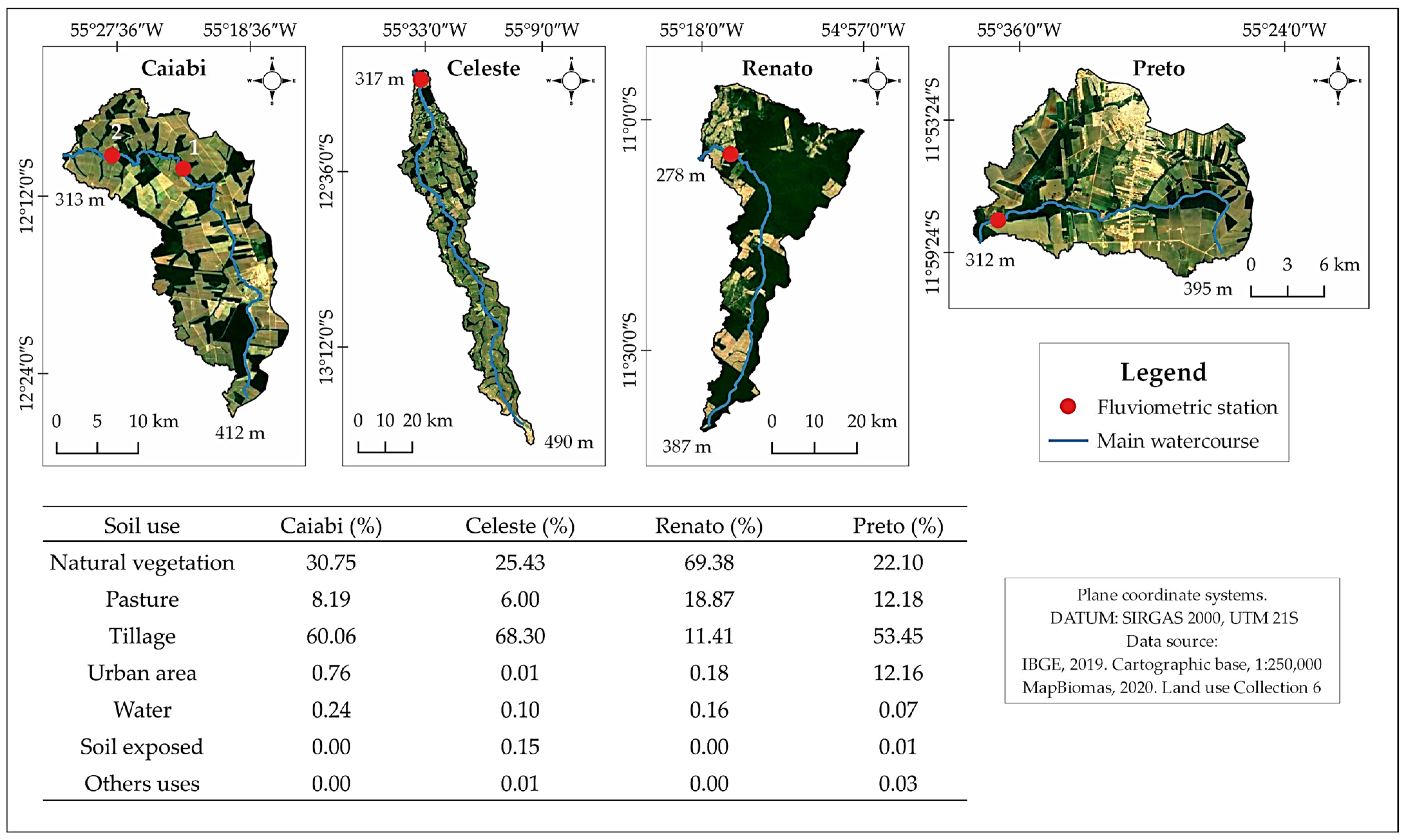
Our study area corresponds to the sub-basins within the Teles Pires River basin, located between 7°16′47″ and 14°55′17″ S and longitudes 53°49′46″ and 58°7′58″ W covering the territories of the states of Mato Grosso and Pará, Brazil. The drainage area of the watershed is approximately 141,278.0 km² and the length of the main watercourse is approximately 1498 km. The Teles Pires River basin has predominant vegetation cover of Cerrado (Upper Teles Pires), a Cerrado–Amazon transition zone (Upper and Middle Teles Pires) and Amazon (Middle and Lower Teles Pires) biomes (Figure 1). Currently, this basin is inserted in the agribusiness hub region of Mato Grosso, with a predominance of agricultural activities, followed by hydroelectric and industrial projects.

The climate of the study region (Cerrado-Amazon transition) is Aw (tropical hot and humid), with climate seasonality defined by two hydrological seasons, the rainy season (October–April) and the dry season (May–September). The mean annual precipitation was 1970 mm, concentrating more than 1700 mm in the rainy season, the reference evapotranspiration ranges from 84 to 131 mm month⁻¹, between the rainy and dry periods of the region, respectively, and the mean annual temperature varies from 24 to 27 °C [34].

The definition of the five cross-sections for fluviometric monitoring followed the following criteria: ease of access and logistics, site free of anthropic actions, stretch with well-distributed speeds, bed and stable margin, well defined and free of vegetation, rocks and other obstacles, rectilinear stretch with parallel margins, regular longitudinal profile and free of backwaters and location far from confluences, location with adequate conditions for the installation, maintenance, and operation of equipment [35].

The general information of the fluviometric stations is presented in

Table 1. General characteristics of the Teles Pires River basin sub-basins, Mato Grosso, Brazil.

Sub-Basin	Fluviometric Station	Latitude	Longitude	Altitude (m)	Subarea (km2)	Main Watercourse (km)	Period of Data
Caiabi	Caiabi 1	12°10′32.64″ S	55°23′5.22″ W	372	340	40	December 2020–September 2021
	Caiabi 2	12°09′27.23″ S	55°28′30.39″ W	345	454	53	March 2020–September 2021
Celeste	Celeste	12°17′39.02″ S	55°33′56.90″ W	319	1.788	211	August 2020–October 2021
Preto	Preto	11°58′1.51″ S	55°37′20.25″ W	325	243	25	May 2020–September 2021
Renato	Renato	11°4′6.29″ S	55°14′59.05″ W	281	1.181	80	April 2020–June 2021

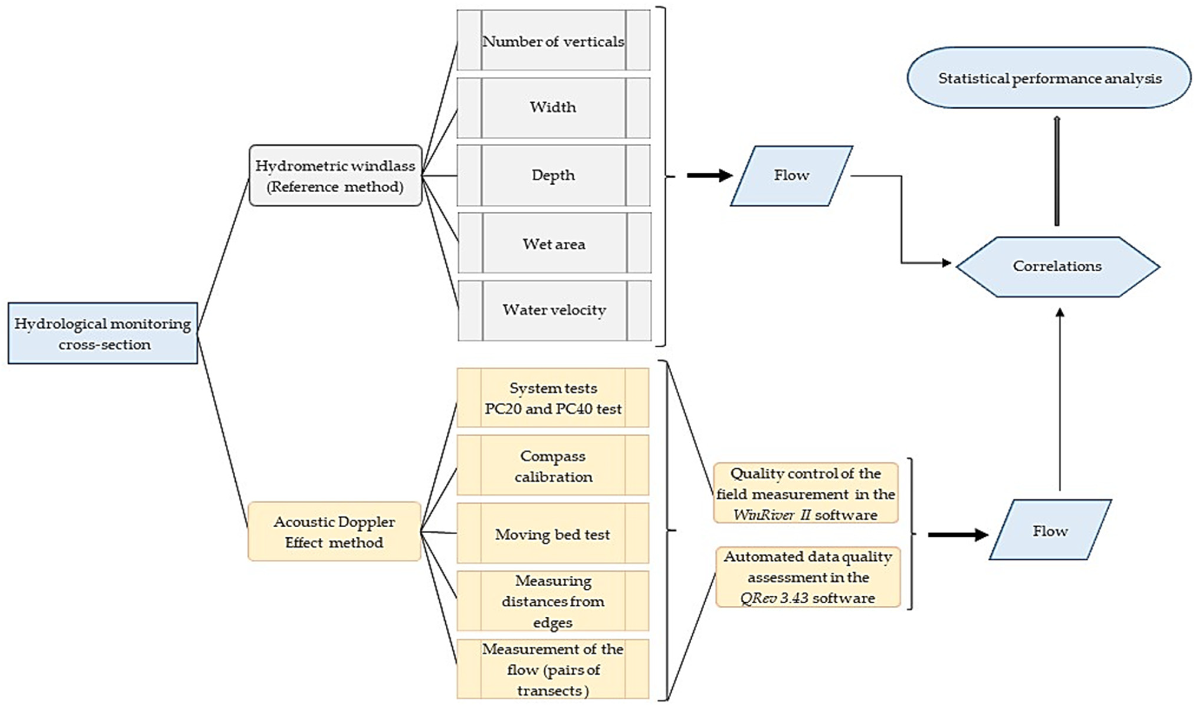
. The areas of the hydrographic sub-basins of the Caiabi, Celeste, and Preto Rivers present a predominance of agricultural activities, with the cultivation of soybeans, corn, cotton, and beans and a considerable urban occupation in the Preto River area. In contrast, in the Renato River area, native vegetation and livestock are predominant, with a significant rise in agriculture (Figure 2). The flowchart of the field measurement steps and subsequent analyses carried out on the collected data are presented in Figure 3.

2.2. Measurements of Depth and Flow by the Reference Method

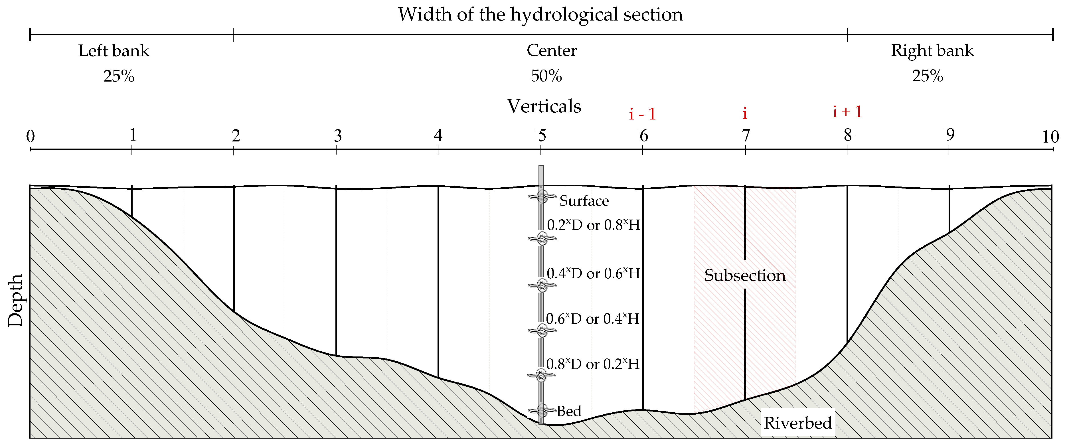
Each monitoring cross-section was demarcated with a graded string fixed between the channel margins and then divided into subsections, represented by fixed verticals, positioned longitudinally along the section [35]. The distance between verticals and the number of verticals was defined according to the width of each cross-section (

Table 2. Distance between fixed verticals according to the width of the river cross-section.

Width of the River (m)	Distance between Verticals (m)
<3	0.3
3–6	0.5
6–15	1
15–30	2
30– 50	3
50–80	4
80–150	6
150–250	8
>250	12

Note: Source: [33].

). In contrast, the position and number of reading points were determined from the depth measurement of each vertical (

Table 3. Depth, number, and position of points on the measuring vertical and calculation of the mean velocity for the respective vertical.

Depth (m)	N° of Points	Position of the Points	Mean Velocity in the Vertical
0.15 to 0.60	1	0.6 D	V0.6
0.60 to 1.20	2	0.2 and 0.8 D	(V0.2 + V0.8)/2
1.20 to 2.00	3	0.2; 0.6 and 0.8 D	(V0.2 + 2 × V0.6 + V0.8)/4
2.00 to 4.00	4	0.2; 0.4; 0.6 and 0.8 D	(V0.2 + 2 × V0.4 + 2 × V0.6 + V0.8)/6
>4.00	6	S; 0.2; 0.4; 0.6; 0.8 D and B	[VS + 2 × (V0.2 + V0.4 + V0.6 + V0.8) + VB]/10

Note: D is the depth of river (m); S is the point very close to the surface; B is the point very close to the bed. Source: [33].

) [35]. The position and number of verticals and measuring points may vary according to the year’s water season, which is necessary to measure the width and depth of the fluviometric cross-sections at each field campaign (Figure 4).

The reference bathymetric survey of each cross-section was carried out from the direct measurement of the depth in each vertical. Sections with a depth of less than 2.50 m were measured at hand, with a metallic rod graduated with a numerical scale of 0.01 m, the reference being the riverbed (obtaining H—height of the water column over the point). For sections with a depth greater than 2.50 m, we use a GFL-25 fluviometric winch and a LAS-15 fluviometric ballast (15 kg model), manufactured by JCTM Ltd.a, in Rio de Janeiro city, Brazil, both installed on an aluminum boat. In this method, the water surface is the reference, and an analog odometer is used, which must be reset with the central axis of the hydrometric windlass level with the water surface and then submerged to the riverbed to obtain D (depth) of the water vertical.

Water velocity measurements to obtain flow were performed by direct measurement with a hydrometric windlass manufactured by JCTM Ltd.a, model MLN-7, in Rio de Janeiro city, Brazil, associated with an electronic revolution counter, connected together. In this case, the metal propeller rotates in the opposite direction of the flow under the action of the movement of the water in the river and sends electrical signals to the rotation counter, which relates the number of rotations per second with the flow velocity.

During measurements, the equipment was positioned with the propeller against the direction of the water flow and three readings of the number of rotations were performed for a time of 40 s per reading, considering a standard deviation ≤10%, in each position of each vertical of the cross-section, from the left bank to the right bank. To obtain the average speed in each vertical, the rotations were converted into speeds through the linear equation established by the manufacturer. The time of 40 s per reading was sufficient for average conditions of regular flow in all sections evaluated [35].

The wet area of influence of each cross-section was calculated using the numerical method of the half section or subsection (Figure 4), which consists of calculating the partial flows of each subsection by multiplying the average velocity of the vertical by the area of the trapezoidal segment, defined by the product of the average depth by the sum of the semi-distances to the adjacent verticals [35]. This method disregards the areas close to the margins (Equation (1)):

$${\mathrm{A}}_{\mathrm{i}}=\frac{\left(\frac{{\mathrm{D}}_{\mathrm{i}-1}+{\mathrm{D}}_{\mathrm{i}}}{2}+{\mathrm{D}}_{\mathrm{i}}\right)}{2}·\frac{\left({\mathrm{d}}_{\mathrm{i}}-{\mathrm{d}}_{\mathrm{i}-1}\right)}{2}+\frac{\left({\mathrm{D}}_{\mathrm{i}}+\frac{{\mathrm{D}}_{\mathrm{i}+1}+{\mathrm{D}}_{\mathrm{i}}}{2}\right)}{2}·\frac{\left({\mathrm{d}}_{\mathrm{i}+1}-{\mathrm{d}}_{\mathrm{i}}\right)}{2}$$

(1)

where D_i−1 is the depth of the vertical preceding the vertical whose area of influence is being calculated (m); D_i is the depth of the vertical whose area of influence is being calculated (m); D_i+1 is the depth of the vertical behind the vertical whose influence area is being calculated (m); d_i − d_i−1 is the distance between the vertical whose area of influence is being calculated and the previous vertical (m); d_i+1 − d_i is the distance between the vertical whose area of influence and the posterior vertical is being calculated (m) (Figure 4).

The total net flow for each cross-section was determined by the sum of the product of the velocity and the wetted area of each subsection (Equation (2)).

$${\mathrm{Q}}_{\mathrm{L}}=⅀{\mathrm{q}}_{\mathrm{i}}=⅀({\mathrm{V}}_{\mathrm{i}}\times {\mathrm{A}}_{\mathrm{i}})$$

(2)

where Q_L is the total net flow (m³ s⁻¹); q_i is the flow of each subsection (m³ s⁻¹); V_i is the average velocity of the vertical (m s⁻¹); and A_i is the wetted area of the subsection (m²).

2.3. Measurements of Depth and Flow by the Acoustic Doppler Effect Method

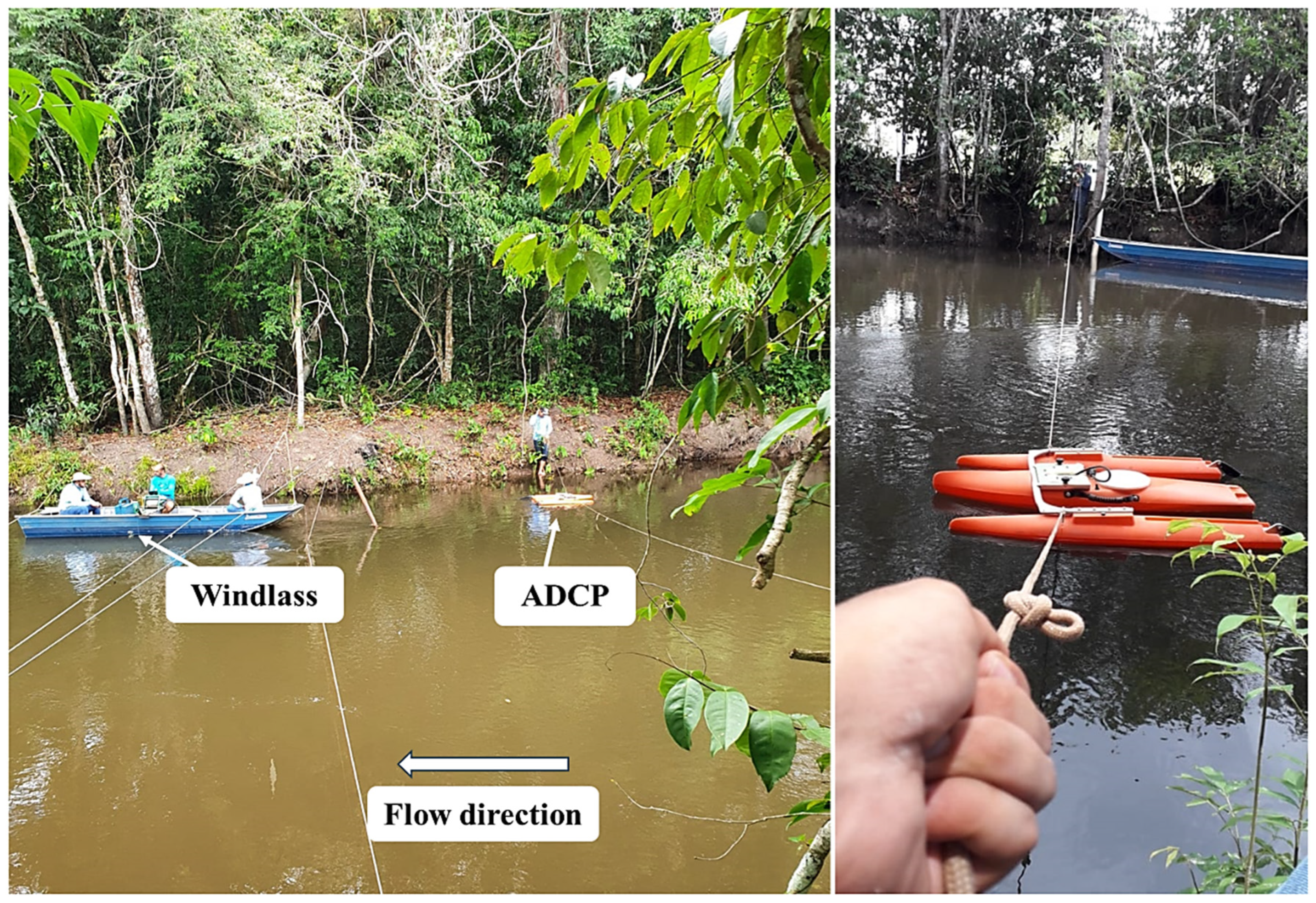
In addition to the measurements with the hydrometric windlass (reference method), a bathymetric survey and water velocity measurements were carried out by indirect measurement to obtain the flow of five cross-sections for monitoring with the Doppler Acoustic Current Profiler (ADCP model RiverRay manufactured by Teledyne Marine RD Instruments, Poway City, CA, USA). This equipment consists of a transducer with two pairs of beams, standard temperature, pressure, inclination, acoustic depth and internal compass sensors, a 12 V battery, and a trimaran for its operation (the GPS was not coupled to the ADCP).

The ADCP RiverRay is a robust equipment that measures the speed of propagation of a sound wave emitted and reflected by particles suspended in water, converting these sound waves into electrical signals interpreted by the WinRiver II 2.18 acquisition software. The transducer performs readings in the vertical orientation, which makes it more accurate for detailed bathymetric surveys, emitting and receiving sound signals with a frequency of 600 kHz ranging from 300 to 3000 kHz, and estimation of water velocity with a range of background pulse between 0.4 and 60 m [26,37].

The basic settings of file preparation, as well as the system tests, compass calibration, moving bed test, and depth and flow measurements, were carried out in the WinRiver II 2.18 data acquisition software. The information was transmitted via Bluetooth from the notebook between the ADCP and the software.

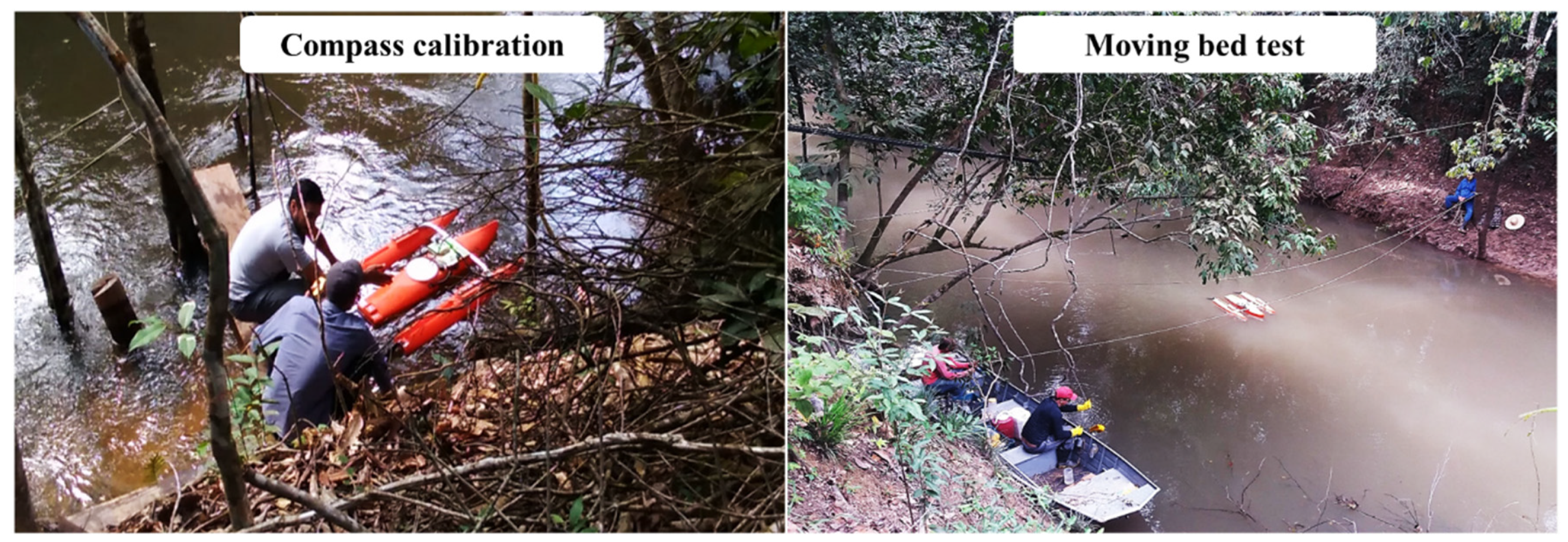
They initially used this software to run the PC20 and PC40 system test protocols. Next, the compass calibration was performed, which consisted of slowly turning the ADCP clockwise by 360° with the transducer in contact with the water, adding a minimum time of 3 min for the complete turn; at this stage, at least 100 assessments must be performed during a complete rotation. In each measurement for each cross-section, the stationary, moving bed test was performed by the mean subsection method in a minimum time of 600 s (~10 min); in this case, the equipment was positioned in the center of the cross-section and fixed with two taut ropes between the edges of the section, seeking to avoid the occurrence of vibrations as much as possible [37]. The result of this test is analyzed in the data post-processing step (Figure 5).

The bathymetric survey was carried out concomitantly with the flow measurement. The ADCP was positioned with the front of the trimaran against the water flow direction and at a profiling depth of 0.10 m. Two operators guided the crossing of the ADCP, positioned one on each river bank with the aid of two ropes fixed on each side of the trimaran, at a constant speed and lower than the water velocity. The measurement started from the left bank to the right bank, covering a continuous transect, parallel and upstream of the section in which the flow measurement was carried out with the hydrometric windlass (reference method) with an approximate distance of 2.5 m between the parallel sections (Figure 6).

The first reading begins with the emission of sound pulses “pings”, registering at least 10 beams with the ADCP stopping on the left bank and ending when counting 10 more beams with the equipment stopping on the right bank. A measurement with ADCP corresponds to a pair of transects, that is, a round trip between the edges of the section (Figure 7). However, strips close to each bank cannot be measured due to restrictions on the presence of roots and shallow banks (depth < 0.3 m), and the size of these strips close to the banks varies according to the width and depth of each cross-section and water season of the year. In this way, these ranges are measured at the beginning of the first reading of each section and inserted in WinRiver II 2.18, so that they can be considered in the extrapolation to obtain the total net flow.

The quality control of the field measurement for each transect followed the criteria pre-established by the United States Geological Survey (USGS) located in Reston city, Virginia, USA, which were observed by the WinRiver II 2.18 software at the time of the field measurements. Thus, for the reading to be valid, one must: (i) count 10 more verticals in each transect at the beginning and end of the measurement of each transect, with static ADCP within the pre-defined limits of the margins; (ii) the width of the measured strip must be greater than 50% of the total width of the cross-section; (iii) compose the minimum time of 720 s adding all the transect pairs, that is, the total measurement; (iv) the measured net flow (Q_L) must be ≥50% of the total net flow (Qt); (v) the percentage of verticals considered bad must be <25% of the total observed; (vi) the verticals considered of poor quality + verticals with lost measurement must be less than 10% of the total number of verticals observed; (vii) the “pitch and roll” must be less than 5° of variation (inclination of the ADCP in the longitudinal and transverse directions of the vessel); (viii) and the ADCP velocity needs to be less than the water velocity (Figure 8) [37]. For the hydrographic sub-basins studied, 10 reading pairs (20 transects) were established per cross-section on each measurement date.

2.4. Processing of Measured Data

The bathymetric survey and flow measurements of the five monitoring cross-sections were analyzed for the consistency and integrity of measurements by both types of equipment. The data obtained in the field by the hydrometric windlass were processed in an electronic spreadsheet, and the data obtained by the ADCP were analyzed using the QRev 3.43 post-processing software developed by USGS [27].

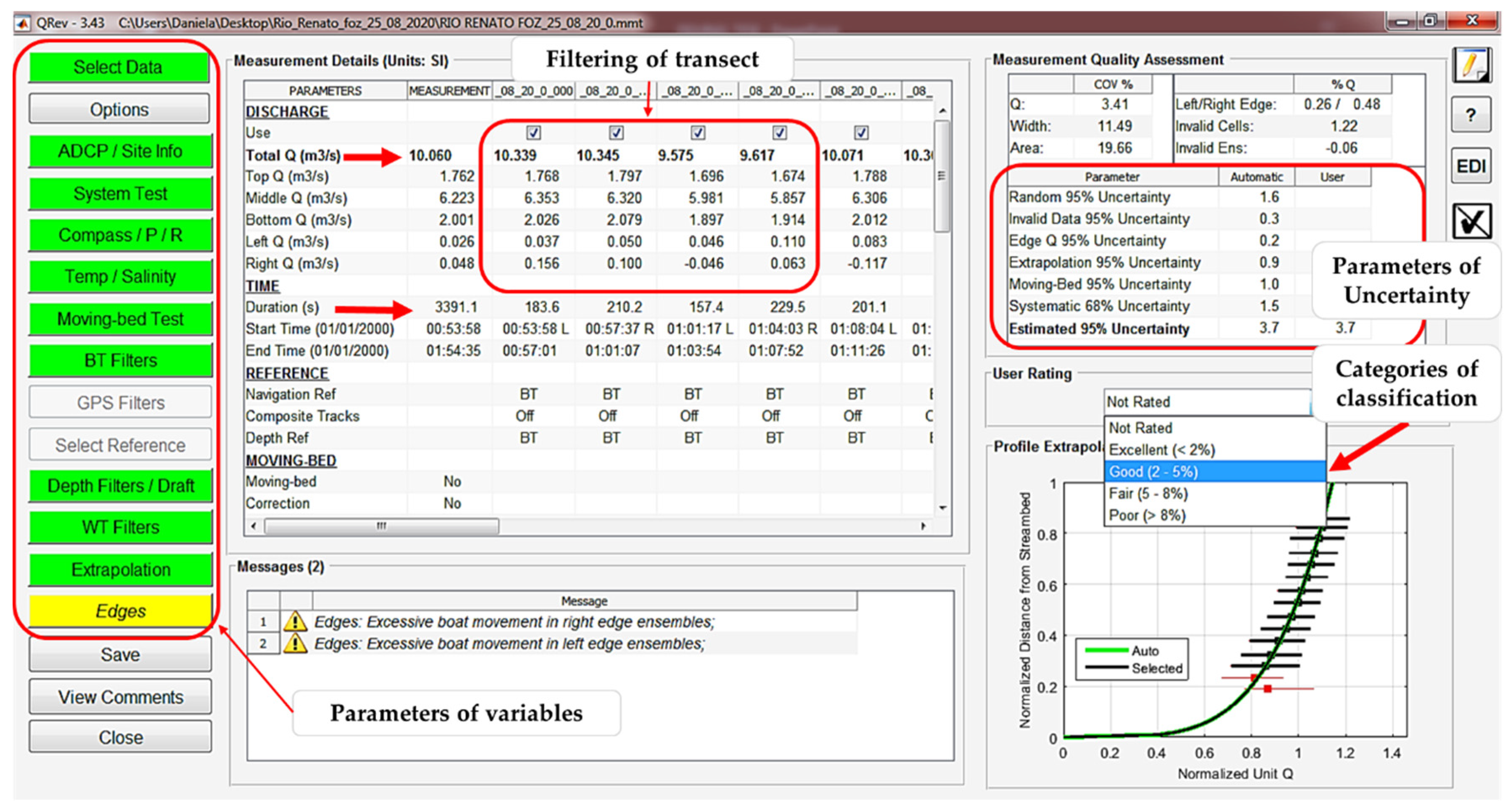
The QRev 3.43 software reviews and processes the data generated by WinRiver II 2.18 using consistent algorithms, applying the so-called automated data quality assessment (ADQA) of parameters of the net flow measured in the field. This software makes it possible to automate the filtering and verification of data quality through graphs and tables containing quality indicators generated in its interface. Thus, the present study decided to work with the standard configurations of extrapolation algorithms in automatic mode.

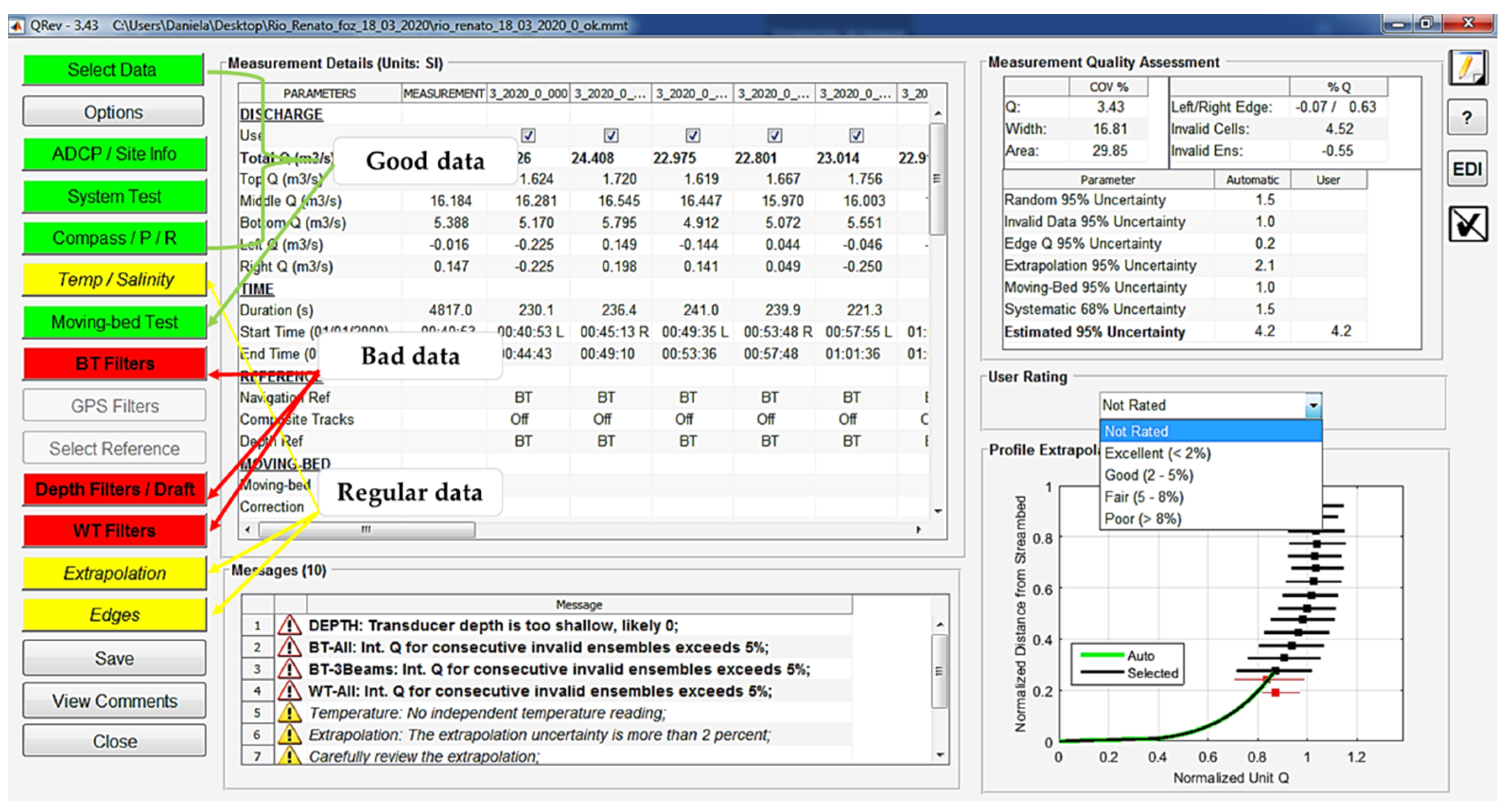
The ADQA considers several parameters/attributes of the measured flow, such as transect parity, minimum total measurement time (720 s), system tests (PC20 and PC40), compass calibration, temperature and salinity, stationary moving bed test, the validity of sets of verticals and cells per transect, transducer depth, extrapolation, and effects of margins on flow (Figure 9). The parameters of a measurement considered “good”, which passes the ADQA, are identified by green color; in a regular measurement with a reading problem, but not critical by ADQA, the yellow color represents them; and bad measurements that do not pass the ADQA, that is, when there are critical reading problems that violate the USGS measurement policies and procedures, are indicated by the color red (Figure 9 and Figure 10).

The QRev 3.43 software also provides data classification categories based on the parameters of random uncertainties, invalid data, edge flow, extrapolation, stationary moving bed test, systematic errors, and, above all, based on estimates, all with 95% confidence level uncertainty. In addition, this allows the user to manually interpret and classify the category of each measurement: excellent (<2%); good (between 2 and 5%); regular (between 5 and 8%); poor (>8%) (Figure 9).

In the present study, a total of 56 measurements (560 pairs of transects) were analyzed in the ADQA and 10 (100 pairs of transects) were excluded due to significant issues regarding statistical uncertainty that violated USGS policies (parameters in red). Of the 10 excluded measurements, 7 were obtained in the dry season and 3 in the rainy season, and the main problems identified were: (i) operational errors such as the system test not being performed; (ii) lack of transducer depth information and consequent errors in flow extrapolation; (iii) ADCP velocity (BT filters) and water velocity (WT filters) reading errors; (iv) bad cell reading and loss of vertical set (Figure 10).

In the user’s evaluation, the rate between 2 and 5% was defined as “good” quality for the estimated data uncertainty. Finally, after the joint evaluation obtained by ADQA and the classification of the estimated uncertainty, 46 measurements (460 pairs of transects) were established for the analysis and estimation of the flow and 46 transects for the depth, obtained both with the metallic rod, windlass, and ADCP. Obtaining the net flows with the ADCP occurred without the global positioning system and salinity sensor; however, the absence of these sensors did not compromise the quality and statistical security of the measurements.

2.5. Analysis and Estimates for Depth and Flow

Depth and discharge measurements by the reference method and with the ADCP were carried out simultaneously at monthly intervals (between March 2020 and October 2021) for the five monitoring cross-sections. From the 46 measurements established in the ADQA for the measurements with the ADCP, the same measurement dates were defined for the metal rod and windlass. The analysis of the flows obtained by the ADCP occurred as follows:

• First, the minimum number of pairs of transects with a minimum duration of 720 s of the total measurement (minimum flow measurement time by ADCP RiverRay established by the USGS) on each measurement date of each cross-section was filtered in QRev 3.43 [37]. Subsequently, other transect pairs were added (one at a time) until the 10 measurement pairs defined in the study were completed. For each pair of incremented transects, the average values (annual) and amplitudes (dry and rainy seasons) of the flow, coefficient of variation, estimated uncertainty, number of pairs, and total measurement time were determined;
• The second part of the analysis consisted of establishing the minimum number of pairs of transects for each cross-section, based on the statistical security given by the uncertainty estimate at a 95% confidence level, defined in this study as a category between 2 and 5% (classified as good). The minimum number of pairs of transects was defined by measurements in the dry season since, in this period of drought, there are more limitations on measurements, such as smaller depths and widths of cross-sections, factors that influence the quality of the ADCP measurements;
• The last step was summarized by relating the average values of the outflows obtained by each set of transect pairs of each cross-section measured by the ADCP with the average values measured by the hydrometric reel, seeking to verify the agreement between the methods of measuring the flow for rivers with low depth.

The analysis of the bathymetric survey obtained by the ADCP occurred as follows:

(i).

In WinRiver II 2.18, a representative transect of each cross-section was defined based on the following observations: a transect whose flow value was close to the average net flow value of the section; a transect that had the minimum number of cells and lost verticals; and transects in which faults or noise interfering in the measurement of the depth of the verticals were absent.

(ii).

In the sequence, the depth values were obtained in punctual verticals and representative of the selected bathymetry, the extraction of the values was carried out manually with the aid of the cursor (mouse) along the transverse profile mapped by the ADCP. At this stage, the objective was to relate the depth values of both methods in the same verticals (subsections);

(iii).

Additionally, the number of verticals per transect, time per transect, time per vertical and the time of the continuous bathymetric survey of the transect at the peaks of maximum and minimum flow were surveyed.

For the net flow, the data were evaluated in the total grouping, monthly measurements between March 2020 and October 2021 by simple linear regression (y = a + bx), between windlass and ADCP. For comparing the bathymetry (fluviometric rod or winch and ADCP), data groups such as total section, margins and center were considered. The databases of the depth and flow variables in all the data above the groups were separated by 70 and 30%, respectively, for the calibration of the coefficients and evaluation of the statistical performance of the generated estimation models. Data separation occurred so that all hydrographic sub-basins and water seasons of the year (rainy and dry seasons) were represented in both data groups (calibration and validation).

In evaluating the performance of the adjusted models, the statistical indicators MBE—mean relative error (Equation (3)), RMSE—square root of mean relative error (Equation (4)), and dw—Willmott concordance index (Equation (5)). The MBE indicator is a measure of systematic errors (or bias) that represents the deviation from the averages and provides information regarding the long-term performance of the model, with negative values indicating underestimation and vice versa; thus, an MBE closer to zero is desired, as it indicates the better performance of the tested model. However, within a dataset, an overestimate cancels out an underestimate [38,39].

The RMSE is the square root of the mean squared error and informs about the real value of the error produced by the model; that is, it provides a value of the level of dispersion the model produces. However, some large errors in the sum can cause significant increases in RMSE values, in addition to not differentiating overestimation from underestimation, as it is a measure of absolute deviation; RMSE is always positive. The lower the values obtained for RMSE, the better the performance of the models. This is an important statistic as it highlights the reliability and repeatability of the model, providing a term-by-term comparison of the actual deviation between predicted and measured values [38,39]. The adjustment index “d” measures the degree to which a model’s predictions are error-free; this index varies from 0 to 1; it represents how much the estimated values adjust with the measured values, with one being in perfect agreement [39,40].

Badescu [39] suggests the application of statistical indicators based on error instead of indicators based on relative errors and that a minimum subset of statistical indicators can be considered for analyzing the performance of a model; among them, the joint analysis of the MBE and RMSE is recommended, and the t-statistic and the Willmott index “d” can also be added to this subset.

$$\mathrm{M}\mathrm{B}\mathrm{E}=\frac{\sum _{\mathrm{i}=1}^{\mathrm{n}}{\mathrm{P}}_{\mathrm{i}}-{\mathrm{O}}_{\mathrm{i}}}{\mathrm{n}}$$

(3)

$$\mathrm{R}\mathrm{M}\mathrm{S}\mathrm{E}={\left[\frac{\sum _{\mathrm{i}=1}^{\mathrm{n}}{\left({\mathrm{P}}_{\mathrm{i}}-{\mathrm{O}}_{\mathrm{i}}\right)}^2}{\mathrm{n}}\right]}^{0.5}$$

(4)

$$\mathrm{d}\mathrm{w}=1-\frac{\sum _{\mathrm{i}=1}^{\mathrm{n}}{\left({\mathrm{P}}_{\mathrm{i}}-{\mathrm{O}}_{\mathrm{i}}\right)}^2}{\sum _{\mathrm{i}=1}^{\mathrm{n}}{\left(\left|{\mathrm{P}}_{\mathrm{i}}^{\prime }-\overline{\mathrm{O}}\right|+\left|{\mathrm{O}}_{\mathrm{i}}^{\prime }-\overline{\mathrm{O}}\right|\right)}^2}$$

(5)

where: ${\mathrm{P}}_{\mathrm{i}}$—estimated values; ${\mathrm{O}}_{\mathrm{i}}$—observed values; n—number of observations; $\left|{\mathrm{P}}_{\mathrm{i}}^{\prime }-\overline{\mathrm{O}}\right|$—absolute value of the difference between the estimated value and the average of the observed values; $\left|{\mathrm{O}}_{\mathrm{i}}^{\prime }-\overline{\mathrm{O}}\right|$—absolute value of the difference between the observed value and the average of the observed values.

3. Results

The studied rivers are natural and perennial channels and show seasonal variations in the volume and velocity of surface runoff flow. The five hydrological cross-sections showed similar hydraulic dynamics between the hydrological stations in the region, with maximum peaks between March and May (rain-dry transition) and minimum points between August and October (dry-rain transition) for the flow and the other hydraulic variables (

Table 4. Hydraulic characteristics obtained by reference methods in the cross-sections of sub-basins of the Teles Pires river, Mato Grosso, Brazil.

Variables		Caiabi 1	Caiabi 2	Preto	Renato	Celeste
Flow (QL) (m3 s−1)	QLmax	8.91	14.58	6.03	24.11	60.78
	QLmean	5.43	7.29	4.69	16.46	30.47
	QLmin	3.63	3.81	3.48	9.18	22.07
Water velocity (V) (m s−1)	Vmax	0.43	0.61	0.23	0.42	0.63
	Vmean	0.35	0.41	0.22	0.37	0.47
	Vmin	0.33	0.32	0.27	0.29	0.38
Wet area (A) (m2)	Amax	20.15	24.47	23.37	54.55	118.61
	Amean	14.41	16.12	19.39	40.33	62.42
	Amin	10.24	11.10	12.25	29.65	53.18
Width (W) (m)	Wmax	9.00	12.50	12.00	19.20	31.30
	Wmean	8.41	11.70	11.22	18.63	25.98
	Wmin	7.80	10.25	9.50	18.00	24.60
Depth (D) (m)	Dmax	3.24	3.04	2.41	3.77	6.34
	Dmean	1.87	1.35	1.69	2.29	2.25
	Dmin	1.02	0.20	0.17	1.18	1.09

Notes: max—maximum value of a single measurement obtained during the rainy season; min—minimum value obtained during the dry season; med—average value of all measurements during the overall period. Observation: Evaluation period between March 2020 and October 2021.

and

Table 5. General characteristics obtained by the acoustic method by Doppler effect—ADCP RiverRay in transverse sections of sub-basins of the Teles Pires River, Mato Grosso, Brazil.

Variables	Caiabi 1	Caiabi 2	Preto	Renato	Celeste
Maximum flow (m3 s−1)	8.16	14.74	6.22	23.03	54.30
Coefficient of variation (%)	5.29	2.44	4.10	2.57	7.68
Estimate 95% uncertainty (%)	4.70	4.30	4.10	4.10	6.60
Number of transect pairs	6	4	8	4	5
Time of total measurement (s)	1640	1353	1668	1946	1326
Number of verticals per transect	188	230	139	392	211
Time per transect (s)	135	165	100	285	127
Time per vertical (s)	1.40	1.40	1.40	1.37	1.67
Mean flow (m3 s−1)	5.17	7.16	4.63	16.04	27.56
Coefficient of variation (%)	5.11	3.50	6.18	3.42	4.86
Estimate 95% uncertainty (%)	4.80	4.50	4.80	4.90	5.20
Number of transect pairs	7	5	9	5	5
Time of total measurement (s)	1541	1120	1910	1627	1565
Number of verticals per transect	180	176	152	263	204
Time per transect (s)	127	119	108	190	144
Time per vertical (s)	1.42	1.49	1.40	1.39	1.42
Minimum flow (m3 s−1)	3.44	4.30	2.66	10.00	20.95
Coefficient of variation (%)	6.78	3.88	6.72	3.55	3.45
Estimate 95% uncertainty (%)	5.10	4.50	4.90	4.40	4.20
Number of transect pairs	7	5	9	5	5
Time of total measurement (s)	1507	1087	1581	1563	1517
Number of verticals per transect	171	178	124	307	218
Time per transect (s)	117	110	90	222	156
Time per vertical (s)	1.46	1.61	1.38	1.38	1.40

Notes: The minimum and maximum values represent a single measurement obtained during the dry and rainy seasons, respectively, and the mean values represent the measurements of the entire evaluated period. Observation: Evaluation period between March 2020 and October 2021.

).

In general, between the reference method (windlass) and the ADCP, the lowest values of the net flow were obtained using the ADCP, but with a low difference in this variable between the methods used, ranging between 0.02 and 6.48 m³ s⁻¹ between the cross-sections. The highest and lowest flow amplitudes obtained between the methods were recorded in the cross-sections of the Celeste and Preto rivers (Table 4 and Table 5). The depths obtained by the reference method (metal rod or fluviometric winch) were 0.17 to 6.34 m between the cross-sections of the Preto and Celeste rivers, respectively, and those obtained with the ADCP were 0.65 and 6.20 m between the Caiabi (fluviometric station 2) and Celeste rivers (Table 4).

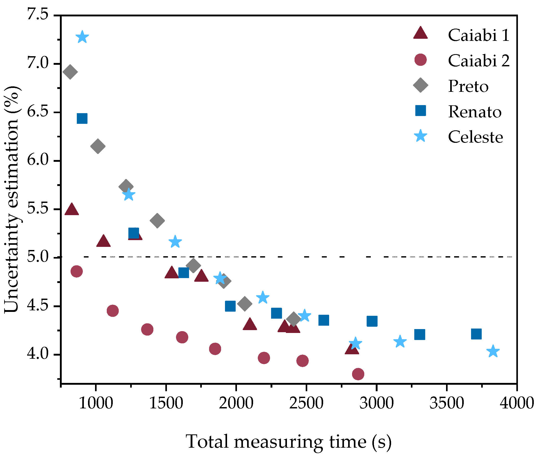
The minimum number of pairs of transects needed to obtain flow measurements with a time greater than 720 s and an uncertainty estimate between 2 and 5% (good quality measurement) in the (dry) period of more limiting conditions was 7 pairs (1507 s) for Caiabi (fluviometric station 1), 5 pairs (1087, 1563 and 1517 s) for Caiabi (fluviometric station 2), Celeste and Renato, and 9 pairs (1581 s) for Preto; under these conditions, the average coefficient of variation ranged from 3.50 to 6.18% between the cross-sections (Table 5). The total measurement time for an uncertainty estimate of less than 5% varied in each cross-section; a reduction in the uncertainty estimate was also observed with the increase in the total measurement time (Figure 11).

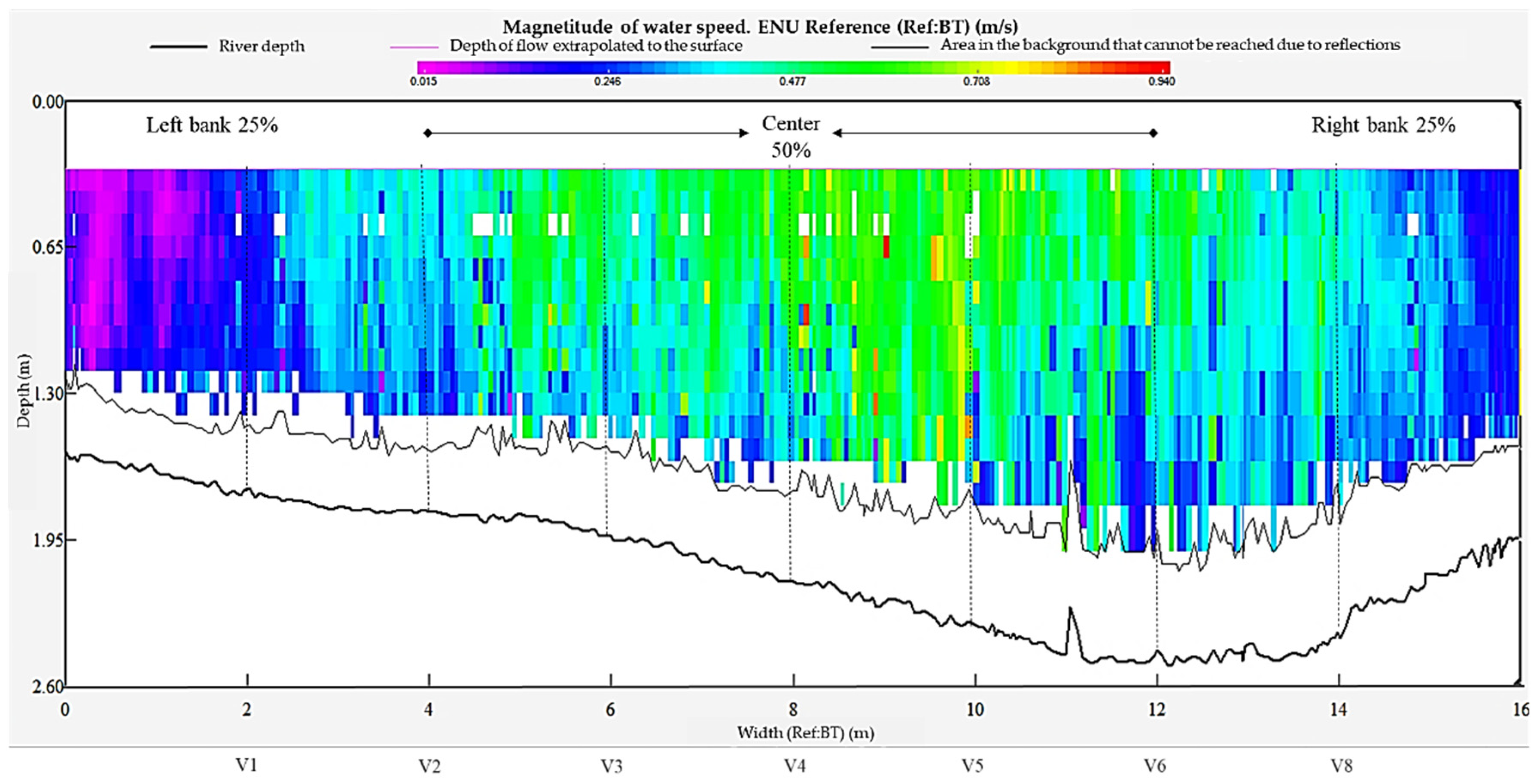
As for the bathymetric profile, the punctual depth of 8–13 verticals was obtained by the reference method according to the width of the cross-section (Figure 12), while by the acoustic method with ADCP, the continuous depth along each section was obtained with an average of 180–263 verticals per transect between cross-sections (Table 5). During the rainy season, with the increase in water level and depth of the cross-sections, “more complete” measurements can be obtained with the ADCP RiverRay, resulting in fewer margins, bed, and surface extrapolations.

The cross-sections studied showed a stable bed and margins, similar in shape to a triangle, with continuous and unidirectional flow but fluctuations in hydraulic variables throughout the year. The water level fluctuated on average by 0.66, 0.87, 0.98, 1.20, and 1.60 m from the average depth for the sections of the Preto stream and Caiabi rivers (fluviometric stations 2 and 1), Renato and Celeste, in that order. The average width ranged from 8.40 to 26.00 m between the cross-sections of the Caiabi (fluviometric station 1) and Celeste rivers, with amplitudes from 1.00 to 6.70 m observed for the same sections between the dry and rainy seasons of the region (Table 4 and Figure 12).

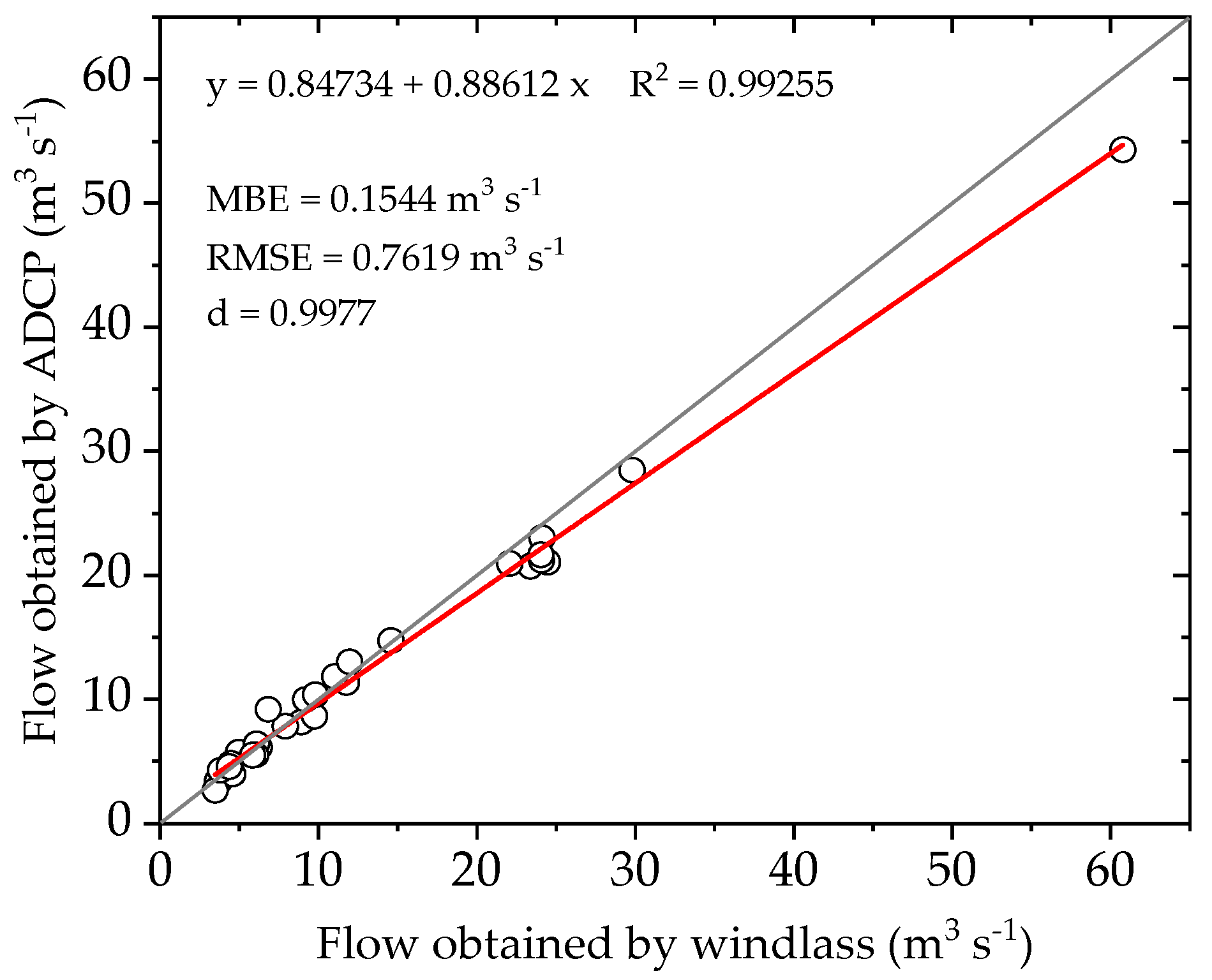
In the relationship between the methods, most of the flows measured by the ADCP RiverRay were underestimated, especially from 15.0 m³ s⁻¹ (Figure 13). The flow estimation equation between the windlass and ADCP showed a satisfactory statistical performance with an adjustment dw of 0.9977. The mean deviation was only 0.15 m³ s⁻¹, which was considered small for the flows obtained in the present study, while the RMSE indicated a strong approximation of the flows measured by both methods (Figure 13).

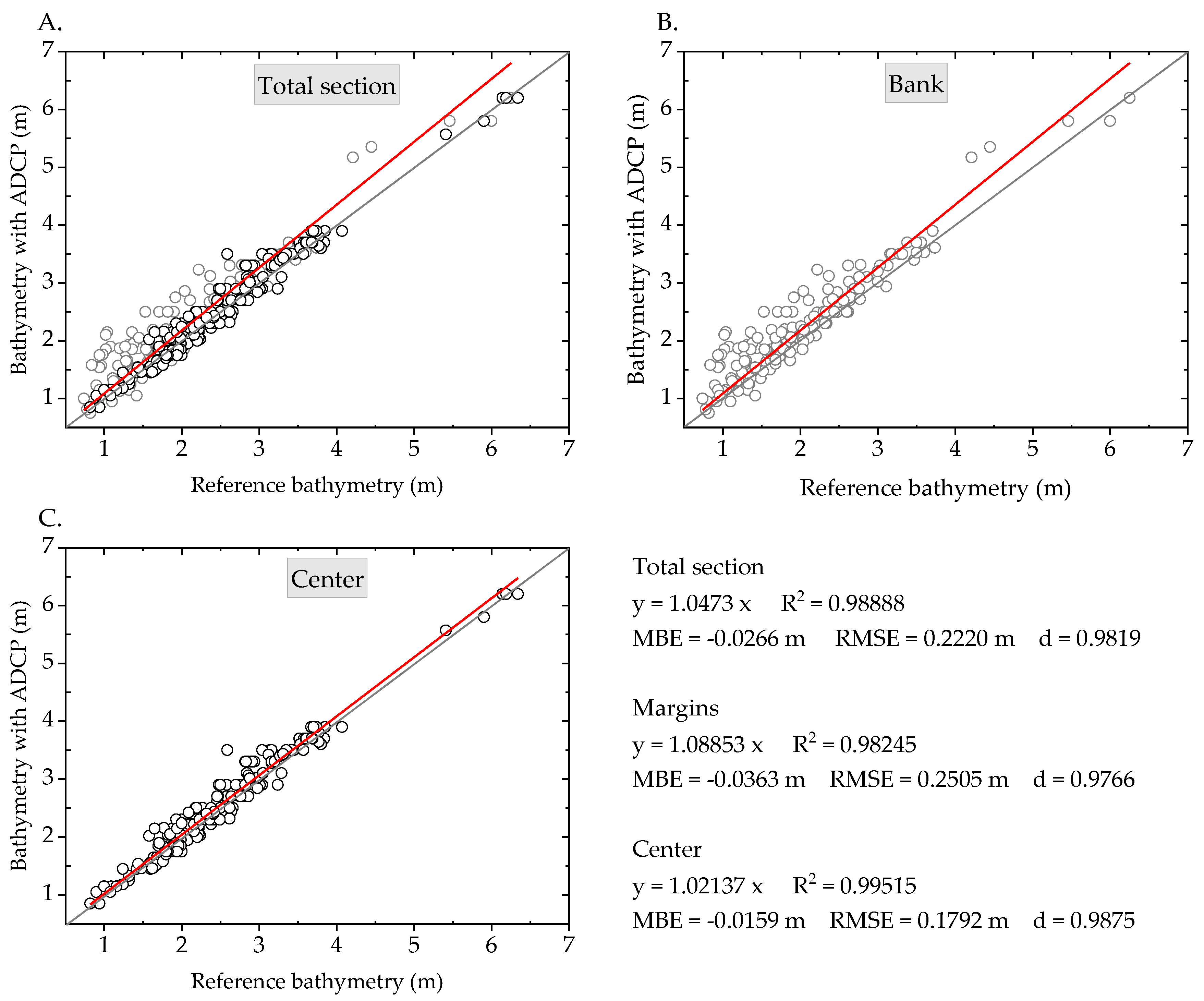
The estimation equations of the depths measured by the reference method and with ADCP RiverRay grouped in the total section, margins and center of the five transversal sections showed a satisfactory performance of the statistical indicatives (Figure 14). Most depth values obtained by ADCPs were overestimated near the margins with differences of 0.37 to 1.11 m and underestimated at the center of the section with differences of 0.34–0.91 m between the evaluated methods. There was a greater mean deviation (4.0 cm) and spread (25.0 cm) of the depth values in the grouping of the margins and smaller in the center of the section (Figure 14).

4. Discussion

The sub-watersheds studied are predominantly rural, the main land uses in these basins are concentrated in rising agriculture and urban/industrial areas (Figure 2). In all cross-sections of the rivers evaluated, the predominant vegetation cover on the banks is native vegetation (Figure 2); however, the amount of cover varies according to the width of the watercourse and the type of vegetation, as established in the Brazilian Forest Code (Federal Law No. 12,651 of 25 May 2012). Soil use and cover conditions are important for evaluating water dynamics in the region’s river basins.

The conditions of soil use and coverage, the density of vegetation cover [41], and the type and physical water characteristics of the soil are important factors that control the dynamics of water and sediments in a river basin [9,42], in addition to climatic [12,29], edaphic [9,43], and physiographic characteristics [13]. The latter refers to the area and density of the drainage network, the shape, slope, and sinuosity of the channel that influence the generation, volume, speed, and direction of the surface runoff flow [42] and the production and transport of sediments [6,7].

The rivers under study are natural and perennial channels with continuous surface runoff flow throughout the year. However, due to regional hydrological seasons, the volume of water drained and sediment transport dynamics vary as the drainage area increases [7]. The survey of water availability in the watercourses of the Caiabi, Celeste, Preto, and Renato rivers is still incipient and recent; only the Caiabi river (fluviometric station 2) has records of net flow by the hydrometric windlass between 5.95 and 16.14 m3 s-1 during the period from December 2018 to February 2020 [44], these values are close to those observed in the present study (Table 4).

The measurement of liquid flow in watercourses can be carried out using different methods and techniques, the choice of which depends on the hydrodynamic and morphological characteristics of the cross-section, the desired precision and accuracy, the availability of equipment, the type and configuration of the equipment, and the operator experience [26,44,45]. The monitoring cross-sections of the present study presented different morphologies; however, the beds (bottom) and margins were stable (Figure 12), maintaining the same conditions observed in another study in this region [7]. The maintenance of the morphological conditions of the sections made it possible to compare the mechanical method with the fluviometric windlass and the acoustic method with the ADCP RiverRay in the on-site measurement of liquid flow and depth.

The largest differences in the net flow measured by the evaluated methods occurred in the cross-sections with higher flows, such as Renato and Celeste (Table 4 and Table 5). Despite these differences, ADCP RiverRay presented a satisfactory statistical performance for measuring the liquid flow in rivers with different depth ranges (0.43–6.34 m) and widths (7.80–31.30 m) in the cross-sections studied (Table 4 and Table 5), in addition to continuously detailing the hydraulic behavior of these sections throughout the year.

Regarding the bathymetric survey, the ADCP measured the lowest depth value (0.65 m) close to the bank, a difference of 0.22 m in terms of the depth measured by the metal rod (0.43 m) on the same shore vertical of the cross-section. This highlights the limitation of ADCP when applied to sections with depths below 0.40 m, and that in this case, the equipment performs extrapolations and interpolations of areas close to unmeasured margins to estimate the depth and velocities of suspended solids and calculate the total liquid flow.

In the acoustic method with ADCP RiverRay, the minimum total measurement time to obtain the net flow in rivers in the Teles Pires river basin mainly depended on the width and speed of the flow, since the wider cross-sections with a higher speed surface runoff flow required a smaller number of transect pairs to complete the minimum time of 720 s required by the USGS (Table 5). Thus, the total measurement time, time per vertical, the number of transect pairs, and the number of verticals per transect depended on the hydraulic characteristics of each hydrological section (Table 4 and Table 5).

The statistical quality of liquid flow measurements must also be considered to establish the total measurement time and the minimum number of transect pairs, as these depend on the quality of the variables obtained during the field measurement. In the present study, based on the uncertainty estimate at 95% confidence, a range between 2 and 5% of the measurement uncertainty was established, which is considered a good quality measurement.

With the increase in the number of transect pairs and the total liquid flow measurement time from the pre-established time of 720 s, the uncertainty estimate decreased by up to 0.5% (Figure 11). Klema et al. [16] reported that the longer a transect is measured, the more accurate the net flow estimate will be, which reinforces the greater influence of the total measurement time in reducing the measurement uncertainty than that of the greater number of transects measured.

In the bathymetric survey, despite finding depths with greater average deviations and scattering close to the margins, when analyzing the grouping in the full section using the reference and acoustic methods using the Doppler effect, it did not negatively affect the quality of the measurement, resulting in a good fit to the equation, and therefore, the bathymetric survey carried out by ADCP RiverRay considered the entire section to be viable to measure the liquid flow (Figure 14).

The fact that the ADCP overestimated the depths as it approached the banks may be associated with the transducer frequency. For the acoustic method using the Doppler effect, the precision of a liquid flow measurement depends on the frequency of the transducer, the mode of operation, and the type of acoustic processing [26,46]. The RiverRay ADCP features automatic configuration and adaptive measurement methods to optimize the ADCP performance for measuring the water speed, turbulence level and depth, a flat-surface phased-array transducer with larger beam angles, making it more accurate for the bathymetric survey in shallow-to-deep rivers (0.4–60 m) and updated software [37,46].

The differences observed between the measured values of net flow and cross-section depth by the two methods may be associated with the level of detail of the measurement. The reference method (windlass) can be considered “static” and punctual, that is, water speed readings are taken with the equipment stopped at pre-established depths and verticals, similarly occurring by obtaining the depth. The acoustic method can be considered dynamic and continuous, as measurements are carried out with the transducer in motion, allowing complete and detailed mapping (screening) of the water velocity and depth of the section in the transverse direction. With this distinction in the level of detail in obtaining the hydraulic variables, the estimated values of the net flow may present differences.

Furthermore, other measurement factors associated with the acoustic method must also be considered and evaluated in situ during measurements to ensure measurement quality, such as errors in the direction and orientation (pitch and roll) of the transducer/profiler during the measurement of water speed, with a vessel speed greater than the water speed, a loss of cells and verticals (bins and beams), changes in the sediment concentration, the presence of plants and roots, dunes, and rocks, high turbulence, bidirectional currents, an error in the ADCP depth (draft), margin errors, analysis error, and a measured liquid flow less than 50% of the total liquid flow, among other errors [26,28,37,47].

The application of the Doppler effect acoustic method with the ADCP RiverRay is a viable alternative for measuring the liquid flow of natural rivers with depths between 0.4 and 6.5 m and widths between 7.80 and 31.50 m; however, care must be taken when applying this equipment when the hydrodynamic and morphological characteristics of the cross-section are not known, it is first advisable to seek to know the hydraulic conditions of the watercourse to choose the most appropriate ADCP configuration for such conditions. It is worth highlighting that the shape of the cross-section is responsible for its hydraulic geometry and influence, above all, the directions taken by surface flow. Furthermore, geomorphological formation can affect the stability of the bed and banks of a channel [13]. Furthermore, the total measurement time of the liquid flow must also be considered to obtain accurate and precise measurements.

Future work will make it possible to compare methods and techniques for measuring the net flow in shallow natural rivers (up to 6.5 m) in the Cerrado–Amazonia transition region, taking into account other geomorphological and physiographic characteristics of the river basin, in addition to analyzing the seasonality of flows during the region’s water regime. Evaluate measurement methods and techniques that optimize human and financial resources and reduce fieldwork time when there is an alternative (non-substitute) and safe method for water and sediment surveying and the monitoring of natural water bodies.

Other studies also report the importance of evaluating measurement methods and techniques for liquid flow and bathymetry [26,46,48,49,50,51,52,53] to define the most appropriate method for measuring and/or estimating the surface flow, as well as understanding the dynamics and availability of water resources, to provide tools that support land use management and the conservation of available natural resources.

5. Conclusions

Measurement with ADCP RiverRay is accurate for obtaining the net flow and depth in shallow cross-sections (up to 6.5 m) of hydrographic sub-basins of the Teles Pires River. Comparisons with the reference method (fluviometric windlass) still need to be evaluated in other shallow rivers with different hydraulic and geomorphological characteristics to optimize and increase the statistical security of measurements in the field.

The increase in the total measurement time greater than 720 s with the use of the ADCP RiverRay influences the reduction in uncertainty in estimating the net flow in shallow cross-sections (up to 6.5 m) of hydrographic sub-basins of the Teles Pires River. Determining the total measurement time and pairs of transects to obtain the measurements of flow depends on the hydraulic characteristics of the watercourse.