Drought Characterization in Croatia Using E-OBS Gridded Data

Abstract

Droughts are among the major natural hazards that are spreading to many parts of the world, with huge multi-dimensional impacts. An extensive analysis of drought phenomenon is presented for continental Croatia based on a meteorological E-OBS gridded dataset (0.25° × 0.25°), within the period of 1950–2022. The drought events were characterized by the Standardized Precipitation Evapotranspiration Index (SPEI), applied to different time-scales (6 and 12 months), in order to describe the subannual and annual variability of drought. The spatiotemporal patterns of drought are obtained through principal component analysis (PCA) and K-means clustering (KMC) applied to the SPEI field. An areal drought evolution analysis and the changes in the frequency of occurrence of the periods under drought conditions were achieved using a kernel occurrence rate estimator (KORE). The modified Mann–Kendall (MMK) test, coupled with the Sen’s slope estimator test, are applied to the SPEI series in order to quantify the drought trends throughout the country. According to the history drought events and considering the different morphoclimatic characteristics of the study area, the results showed that Croatia could be divided into three different and spatially well-defined regions with specific temporal and spatial characteristics of droughts (central northern, eastern and southern regions). A manifest increase is shown in the percentage of area affected by drought, as well as in the yearly drought occurrences rates, in both central northern and eastern regions, and an evident decrease is shown in the southern region for both 6- and 12-month SPEI time-scales. In the observation of the drought’s temporal characteristics, it was found that downward trends expressing increasing drought severities were strongly significant in northern and eastern regions, while a few significant upward trends were seen in the southern region. From this study, it is possible to obtain a broader view of the historical behaviour of droughts in Croatia, with the results providing useful support for drought risk assessment and decision-making processes.

1. Introduction

Droughts are still among the least understood and most complex extreme climate events, affecting large worldwide areas and having serious impacts on society, the environment, and the economy [1]. The Convention to Combat Desertification from the United Nations 15th Conference of Parties (COP15) states in its 2022 report [2] that, globally, the information points in the same direction, which is an increase in the duration and severity of droughts and their impacts on both human societies and ecological systems.

Due to the recent, more pronounced climate variability, drought patterns have been changing, making it more difficult to follow their evolution, which leads to a constant need to update the understanding of their behaviour and characteristics. To better cope with drought, it is also important to distinguish between drought and water scarcity, the two major phenomena that challenge water security [3]: while drought is a natural climate event caused by climate variability that cannot be avoided by water management practices, water scarcity refers to the long-term unsustainable use of water resources, where consumption exceeds water availability, and where water management practices can have an influence [4].

To characterize the drought phenomenon and the occurrence of drought in Croatia, and to understand the historical and recent climate variability in the country, it is important to study the long-term time series of precipitation and temperature, since they show the behaviour of two of the most important climate variables. Around the world, several authors have characterized the phenomenon of drought using well-known scientific indices, such as the Standardized Precipitation Index (SPI) [5] and the more recent Standardized Precipitation Evapotranspiration Index (SPEI) [6], and by studying the spatio-temporal patterns of droughts, along with their duration and frequency.

In this regard, the pioneering work of [7] for the Iberian Peninsula shows that using the SPI at a 12-month temporal scale in 51 monthly precipitation time series within a period from 1910 to 2000 allowed for the identification of four different regions, showing internal homogeneity and well-defined boundaries (north, northeast, southeast and central/western). Specifically for Portugal, and using multiple SPI time-scales, [8] analysed droughts based on monthly precipitation data from a meteorological network, concluding that the country could be divided into three homogeneous regions (north, center and south); the spatial results were confirmed in 2015 by [9] using gridded data and the same drought index. More recently, also based on SPI computed using rainfall grid data for a time window of 100 years, [10] studied regionalized droughts in three regions of Portugal, concluding that the frequency of moderate and severe droughts is increasing. In Southern Europe, [11] studied spatiotemporal drought variation using clustering techniques and the SPEI6 based on gridded datasets, allowing for the identification of five well-distinguished regions in the south of Italy characterized by drought events that differed in terms of their duration and severity. In China, in Xinjiang Province, a study using the Mann–Kendall trend test, cluster analysis and Morlet wavelet analysis concluded that historical drought evolution is better characterized by three regions in close connection with the topography and climate [12]. The recent work of [13] is a good example of climate regionalization, decomposing a field into its spatial and temporal terms, allowing for a study of drought variability in Mozambique.

For the period 1950–2012, in a study about European drought climatologies and trends, [14] found that, in Central Europe and the Balkans, the precipitation increase was not significant, but the temperature increase, and hence the potential evapotranspiration (PET), caused the drought severity to increase. Especially in the last decade, occurrences of drought have been increasing in the Balkans region so that, in 2018–2019, winter precipitation deficits coupled with record-high temperatures in the summer across much of the Balkan Peninsula, i.e., Croatia, Albania, Slovenia, North Macedonia, Montenegro and Hungary, as well as in Slovakia, led to uncommon hydro-climatological conditions that clearly differed from the rest of Europe [15].

It is especially relevant for Croatia that, according to the Center for Climate and Security [16], droughts pose the largest threat to the Balkans region’s stability and prosperity, especially through their impacts on the agriculture and hydroelectric sectors. The western Balkans are also a hotspot of biodiversity in Europe and contain a great diversity of ecosystems, which can be explained by their extremely diverse geology, soil, climate ranges and topography; the Balkans are one of the six European centers of biodiversity [17].

Some studies have been conducted in Croatia regarding drought analysis, namely the works of [18], which applied principal component analysis to a drought index, or [19], which compared the SPI, SPEI, and the standardized groundwater index (SGI) at different time-scales (1, 3, 6, 12, 24, and 48 months). Drought indices (SPI and Palmer Drought Severity Index (PDSI)) were also compared for one meteorological station in north–western Croatia and their agricultural impacts were assessed [20].

In this study, a comprehensive characterization of droughts over Croatia using the SPEI is achieved using the combined classification methods of Principal Component Analysis (PCA) and Cluster Analysis (K-means). The temporal characteristics of drought variability, the changes in the yearly occurrence rate, the drought areal evolution and the characterization of trends via robust and commonly used techniques within the climatology and hydrology fields are examined.

While different studies have been conducted on the Croatian continuum, a long-term analysis aiming to identify the spatial and temporal patterns of drought has never been undertaken. This limitation has largely been due to the unavailability of ground records of climate variables, as the number of meteorological stations with continuous, long time series is relatively small. Therefore, the primary contribution of this research is to address this constraint by utilizing a highly dense, gridded meteorological dataset and employing well-established, validated methodologies to investigate the drought phenomenon across the entirety of Croatia. Importantly, this study represents the first instance in which complete long-term data have been used for this purpose.

The results are intended to be of practical value for planning activities, water resources management, and stakeholders, providing insights that could be used to create risk-based drought management plans at a regional scale but also to understand the connection between drought risk and climate variability.

2. Materials and Methods

By using gridded climate data within a 73-year period, from September 1950 to July 2022, the drought characterization used the following research steps and complementary methods:

(i)

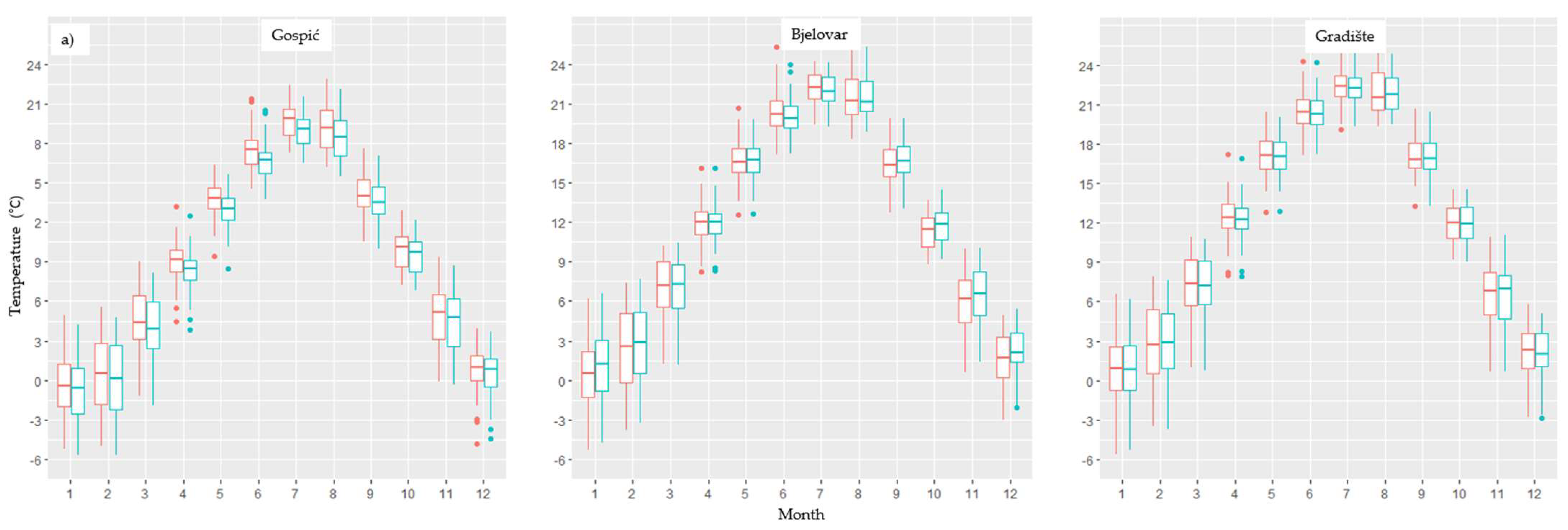
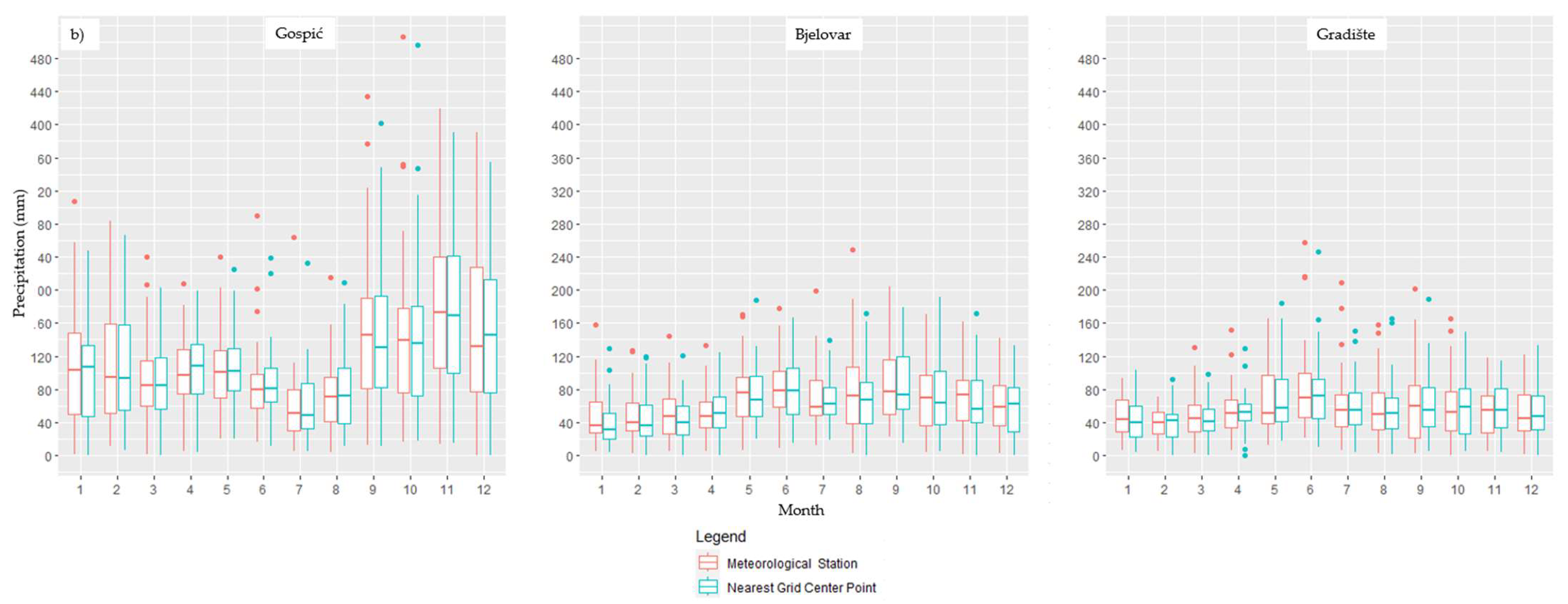
Data validation: E-OBS precipitation and temperature datasets are first validated with records from meteorological stations at different locations in Croatia.

(ii)

Drought index calculation: SPEIs with a 6- and 12-month time-scale (SPEI6 and SPEI12) are calculated to ascertain the sub-annual and annual temporal variability of droughts.

(iii)

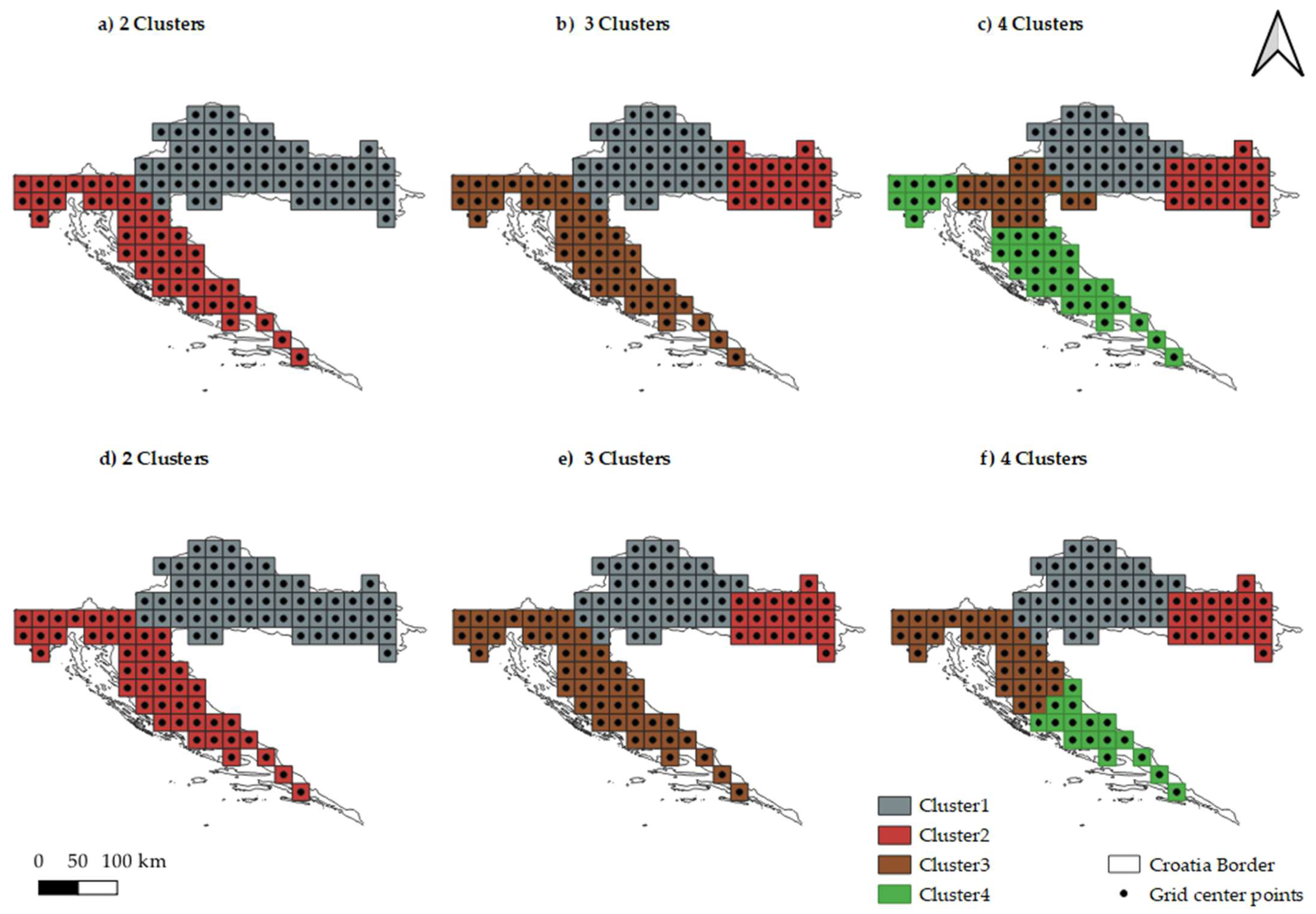
Drought regional patterns: Principal Component Analysis (PCA) was applied to the previous SPEI time series, aiming to identify homogeneous regions. The K-means clustering method (K-means) was used to validate the regions identified from the PCA.

(iv)

Temporal evolution of drought areas: Drought areal evolution of the SPEI6 and SPEI12 fields in each of the identified regions is achieved by assigning an area of influence to each grid cell.

(v)

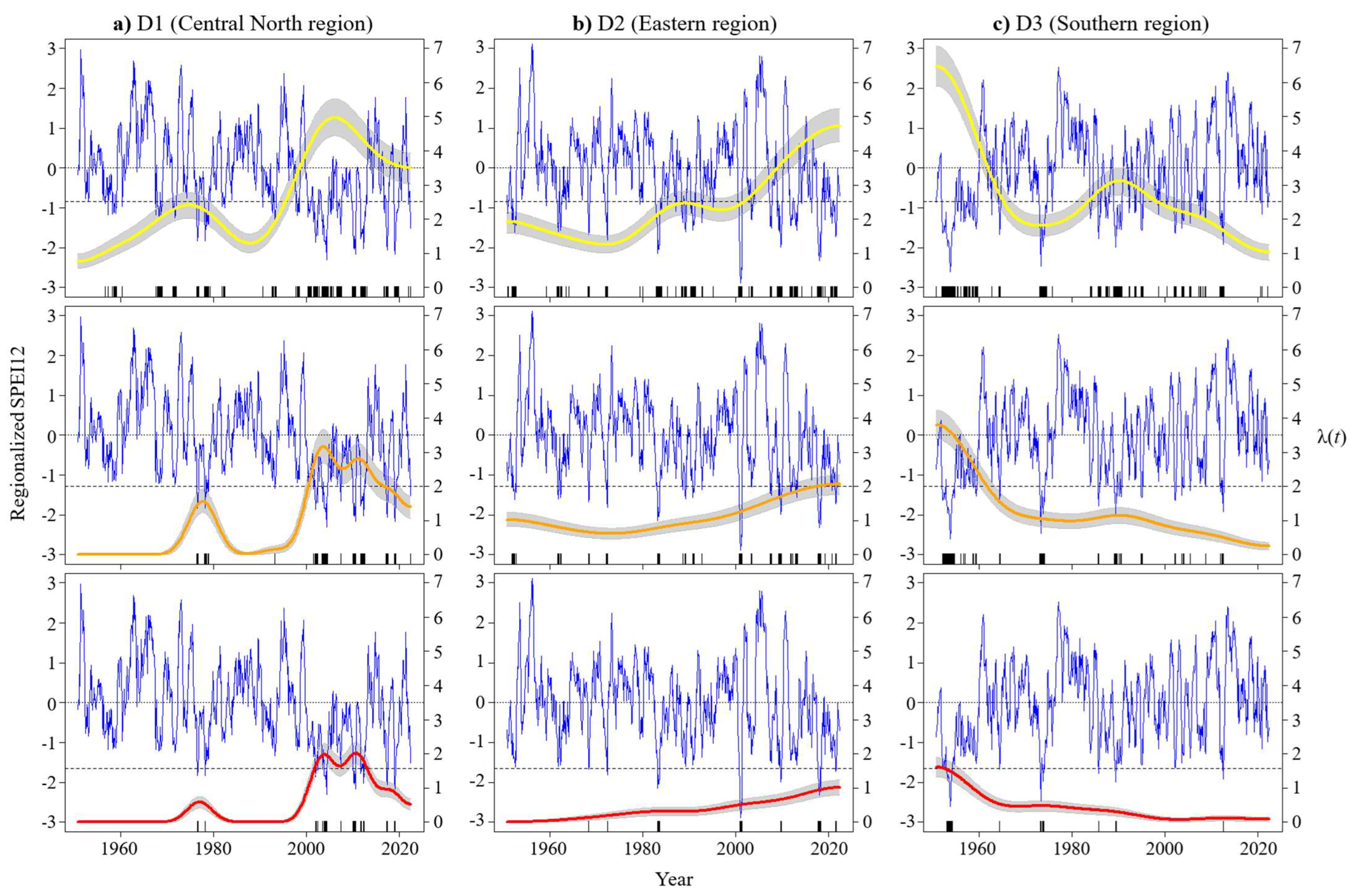
Yearly frequency analysis of drought occurrences: A kernel occurrence rate estimator (KORE) is used to analyse the yearly frequency of the periods under drought conditions for different drought categories according to the regionalized SPEI time series given by the factor scores previously obtained by the PCA.

(vi)

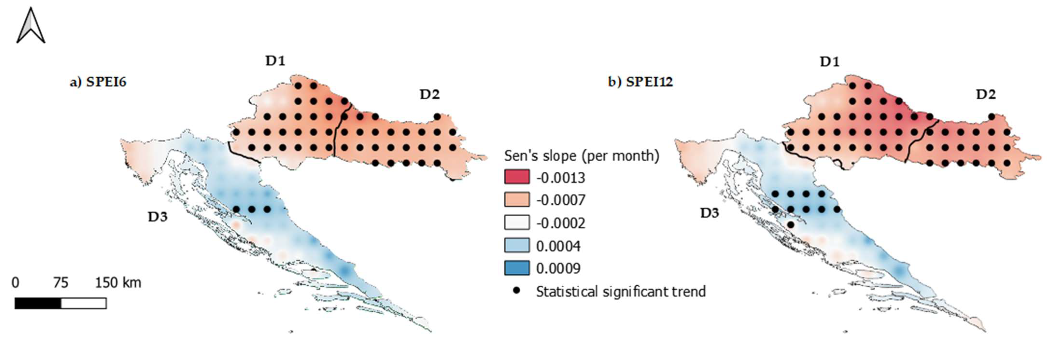
Trend analysis: The Modified Mann–Kendall (MMK) trend test, coupled with the Sen’s Slope estimator test, is used to detect the temporal variability of drought intensities within the SPEI6 and SPEI12 fields in each of the regions.

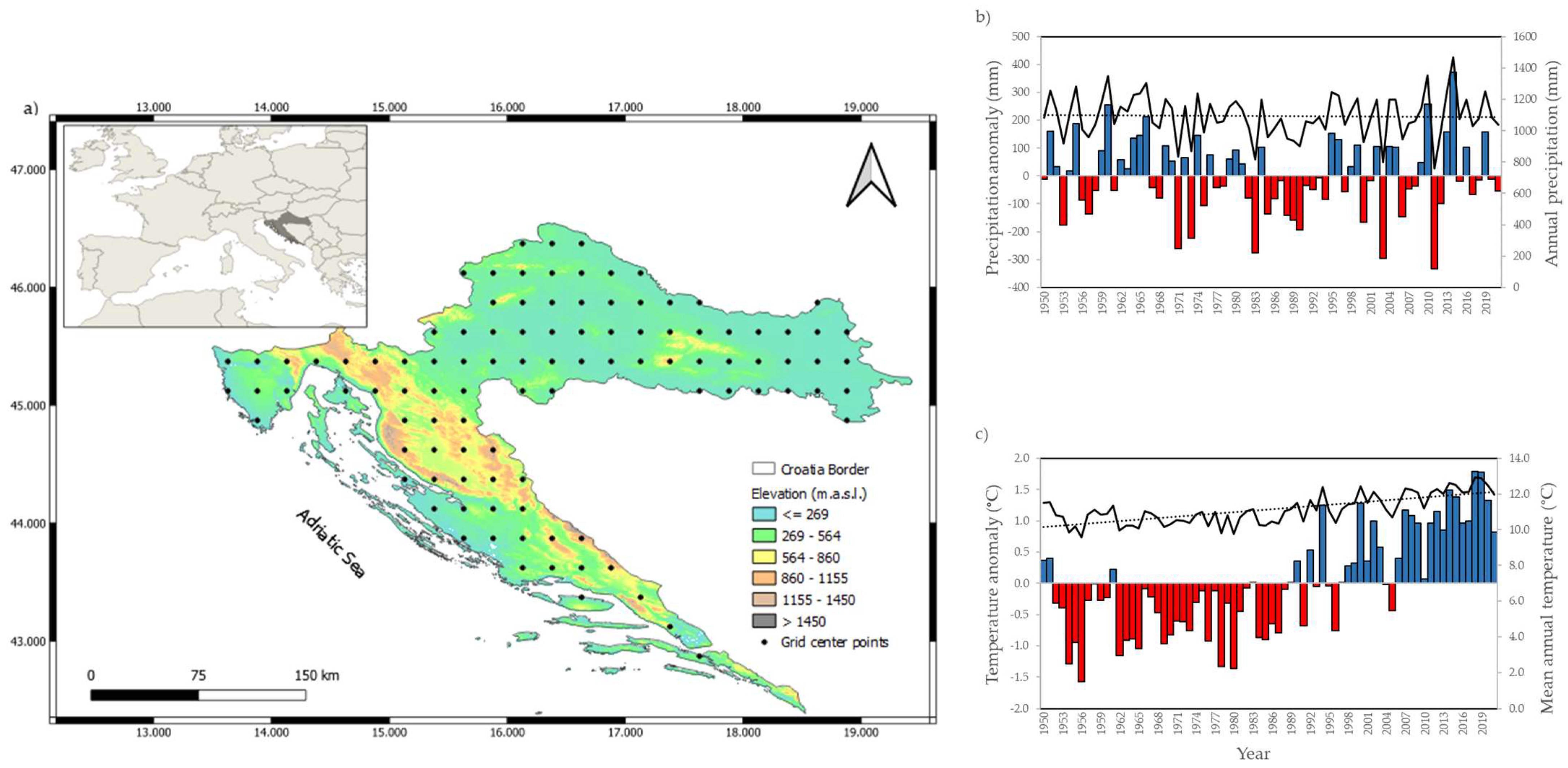
The framework used for the application of the algorithms was developed using the R Software (RStudio Team, 2023), namely by considering the following principal packages: “SPEI” [6], “psych” [21], “modifiedmk” [22], “stats” (developed by the R Core Team and contributors worldwide), and others.

2.1. Study Area

The extensive drought analysis considered mainland Croatia (Figure 1a), approx. 56,594 km², as the study area. The country is located in the middle of the Central and Southeast Europe transition (between latitudes 42° and 47° N and longitudes 13° and 20° E), faces the Adriatic Sea in the southern part and has a complex topography, a complex and variable climate, and diverse terrestrial ecosystems.

The major natural factors that condition the climate of the country are the latitude, the topography, ranging approx. 0–1831 meters above sea level, m.a.s.l. (the highest mountain in Croatia, the Dinaric Alps), and proximity to the Adriatic Sea, with a predominantly Mediterranean influence [23].

The majority of Croatia is characterized by a moderately warm and rainy climate, but it has experienced significant spatial heterogeneity in precipitation with large variability across the country in recent decades [24]. The mean annual precipitation in Croatia is approximately 1100 mm [25] (Figure 1b), ranging from about 3900 mm on the summits of the southern Velebit mountain, located along the northern Croatian Adriatic coast, to about 300 mm on the outlying islands in mid-Adriatic, in close connection with the relief. The mean annual temperature in the lowland area of northern Croatia is 10–12 °C, the mountain regions experience mean temperatures of 3–4 °C, and coastal areas experience temperatures of 12–17 °C [23]. In the last 20–30 years, the average annual temperature has considerably increased over Croatia, where its anomalies reached + 1.8 °C (Figure 1c). A consistent warming trend throughout the whole country was confirmed in recent studies [26]. The precipitation and temperature anomalies in Figure 1b,c represent deviations in relation to the average for the reference period of 1950–2021.

2.2. E-OBS Data

Climate variables, namely precipitation and temperature, were used to calculate the SPEI over a long base period, a 73-year period from September 1950 to July 2022, to correctly sample the natural variability. These were obtained through the Copernicus Climate Change Service (C3S) program, operated on behalf of the European Union by the European Centre for Weather Forecasting (ECMWF). This program combines data from observations of the climate system with recent data and provides high-quality information on the past, present, and future state of the climate for Europe and the World (https://cds.climate.copernicus.eu/cdsapp#!/home; accessed on 25 July 2023). The product used was the “E-OBS daily gridded meteorological data for Europe from 1950 to 2022, derived from in situ observations” (https://www.ecad.eu/dailydata/index.php; accessed on 10 May 2023). This is a daily product for Europe, obtained from observations at stations of the European National Meteorological and Hydrological Services (NMHSs) or other institutions, available on a regular grid of 0.25° × 0.25° [27]. Figure 1a represents the location of the center points of the respective grid.

The monthly time series needed to compute the SPEI for Croatia were generated from the daily temperature and precipitation E-OBS grid datasets by averaging or aggregating daily data into a monthly time-scale, respectively. The resulting grid spatially covered Croatia with 103 grid cells, all within the Croatian border. The 0.25° × 0.25° spatial resolution means a vertical distance that varies with latitude, ranging from 27,660 m in the grid cell of the most southern point to 27,814 m in the topmost northern grid cell. In order to validate the E-OBS grid dataset, the meteorological station data from the Croatian Meteorological and Hydrological Service (DHMZ) were used, and the monthly boxplots between each station and the nearest grid center point were obtained for both climate variables. For this purpose, a common period with available ground data, spanning from 1981 to 2022, was adopted (Figure 2).

The chosen meteorological stations represent Croatian climate zones: the cool temperate moist mountainous regions, close to the Adriatic Sea (Gospić); the warm temperate moist northern central region (Bjelovar); the warm temperate dry northeastern region (Gradište). The grid center point (E-OBS cells) that was assigned, for comparison purposes, to each of the previous stations was the nearest one, which resulted in a maximum distance of 8000 m from the coupled station. The respective elevations from each data source location were also quite similar, reinforcing the comparison between datasets.

From Figure 2, it is clear that both datasets showed similar behaviour through all the months. The central tendency median and similar monthly variability were compared using the equivalent interquartile range. The monthly mean temperatures show the normal yearly distribution of a temperate northern hemisphere country, with the hotter months being those of summer and the colder ones occurring in winter. The within-the-year temporal pattern of the precipitation is always very smooth. The highest values relate to November in Gospić, September in Bjelovar and June in Gradište, for the period 1981–2022.

The Pearson correlation coefficients for the sequential monthly time series of the meteorological stations, and the respective nearest grid center points, were obtained in order to complement the boxplot information; these were 0.98, 0.86 and 0.87 for precipitation in Gospić, Bjelovar and Gradište, respectively, and 0.99 for the mean temperatures in any of the stations.

2.3. Drought Index

The Standardized Precipitation Evapotranspiration Index (SPEI), developed by [6] was adopted as the climate drought index to assess the occurrence of drought in mainland Croatia. The SPEI has become one of the most popular drought indices for drought monitoring, characterization and forecasting [13,15,28,29,30], and is also recognized by the World Meteorological Organization (WMO) as an eligible index for those purposes [31]. It was derived from the original Standardized Precipitation Index (SPI) [5] by accounting for evapotranspiration, and it uses the water balance (WB = P − PET) time series, where P accounts for precipitation and PET accounts for the potential evapotranspiration, instead of precipitation alone, as in the SPI.

As the original formulation of the SPEI suggested, the PET method considered here was the Thornthwaite model, because of the simple data requirements for its computation, which is uniquely based on monthly mean temperatures and the latitude of such meteorological observations [28]. The SPEI has several advantages: (1) great flexibility, as it can be applied at different time-scales, allowing for the representation of the response of crops, natural vegetation and hydrological systems to drought conditions; (2) less complexity than other indices, as it requires relatively simple and well set calculations; (3) great suitability to spatial representation, allowing for comparison between areas within the same region, as it is a normalized index; (4) in comparison with SPI, the SPEI considers air temperature as the most prominent variable of the water budget at the watershed level and most prominent variable of climate change.

The model uses a probability distribution function to fit either the monthly WB series or the aggregated WB over n months for SPEI time-scales higher than 1 month; then, those probabilities are standardized in z units (mean = 0, standard deviation = 1) by a equiprobability transformation and the SPEI time series is obtained. According to [6], the log-logistic distribution adopted here provided better results than other distributions for obtaining SPEI series and has been widely used in many different drought research frameworks and countries [15,32,33,34].

The log-logistic distribution for a given variable x is given by:

$$\mathit{F}\left(\mathit{x}\right)={\left[\mathbf{1}+{\left(\frac{\mathit{\alpha }}{\mathit{x}-\mathit{\gamma }}\right)}^{\mathit{\beta }}\right]}^{-\mathbf{1}}$$

(1)

where α, β, and γ represent the scale, shape and location parameters that are estimated from the x sample (in this case, WB).

When computing the SPEI series, the drought categories adopted for analysis follow the ones proposed by [33], as shown in

Table 1. Drought categories—SPEI values according to [33].

Nonexceedance Probability	SPEI	Drought Category
0.05	>1.65	Extremely wet
0.1	>1.28	Severely wet
0.2	>0.84	Moderately wet
0.6	>−0.84 and <0.84	Normal
0.2	<−0.84	Moderate drought
0.1	<−1.28	Severe drought
0.05	<−1.65	Extreme drought

.

The time-scale of SPEI could be separated into three groups: short (2–4 months), medium (6–10 months) and long (10–20 months) [34]. Normally, short-to-medium SPEI time-scales could be used to analyze the response of crops and natural vegetation to drought, and with longer time-scales, the index could capture water resources’ availability and hence be used to evaluate hydrological variations. In order to characterize the historical drought conditions in Croatia, medium (6 month) and longer (12 months) time-scales were chosen, which allowed for an analysis of the subannual and annual variability in drought conditions (SPEI6 and SPEI12).

2.4. Drought Regional Patterns

To characterize the spatial and temporal drought patterns, principal component analysis (PCA) and nonhierarchical clustering (K-means) were applied to the SPEI time series, as considered by many other authors for drought regionalization purposes [9,10,12,35].

The PCA allows for the classification of data in such a way that the spatial patterns identified for climate data could be expressed in order to highlight their similarities and differences [36]. The original intercorrelated field of SPEI could be reduced to small groups of new SPEI grid center points that are linearly uncorrelated and that explain most of the total variance. The main advantages of PCA [37] are as follows: (1) PCAs are not affected by the lack of independence in the original variables; (2) the normality of the data is preferred but not essential; (3) only an excessive number of zeros would cause problems, which, given the nature of SPEI, is not a concern.

The number of PCs identified by the scree plot method to retain [38] should explain at least 75% of the accumulated variance in the SPEI field. With the main PCs selected, it is possible to produce a more stable spatial patterns by rotating the PCs with the Varimax procedure, providing a clearer division between components due to the redistribution of the explained variance, preserving their orthogonality and producing more physically explainable patterns [39,40,41]. The new elements are referred to as rotated principal components (RPCs).

The PC results can be based on the eigenvalues, the correlations between PCs and the original variables (factor loadings), or the observation coordinates in the PC, which are linear combinations of all the grid point series (factor scores). In order to identify spatially disjunctive areas within the gridded SPEI field, the mapping of the correlations between the retained RPCs and the original SPEI series was also used to validate the obtained classification, confirming the selection of the optimal number of PCs. Accordingly, whenever a group of grid center points had the highest correlation with an RPC, a new region was delimited.

In order to validate the regional classification obtained by the PCA, a cluster analysis using the k-means method [9,10,14] was also applied to see if the number of regions obtained with K-means is equivalent to those obtained by the PCA. The K-means method, similarly to the PCA, has the ability to divide the dataset into homogeneous and distinct groups with members with similar characteristics [41].

The optimal number of clusters was evaluated by the Euclidean distances between the created clusters, which yields the lowest possible number with the greatest possible homogeneity, as the analysis requires that the number of clusters should be established beforehand. To overcome this aspect, which is considered one of the major unresolved issues in the cluster analysis, the test was repeated by considering several number of clusters, with the Euclidean distances being analysed to ensure maximum heterogeneity between groups [37].

2.5. Drought Yearly Occurrence Rate and Trend Analysis

The analysis of changes in the temporal occurrence rate of droughts is a very important aspect when characterizing their persistence and frequency. To evaluate the frequency of the occurrence of these periods under drought conditions over time, a kernel occurrence rate estimator (KORE) was applied to a historical series of drought events with the aim of estimating how the mean yearly number of drought periods, λ, changes over time; that is, to characterize λ (t). Several authors have also used this for similar purposes, such as [42,43,44,45].

The kernel technique is a nonparametric model developed by [46] for smoothing point process data; in the case of the present application, the occurrence times of periods under drought conditions. It can be formulated as:

$$\widehat{\mathit{\lambda }}(\mathit{t})=\sum _{\mathit{i}=\mathbf{1}}^{\mathit{m}}\mathit{K}\left(\frac{\mathit{t}-{\mathit{T}}_{\mathit{i}}}{\mathit{h}}\right)$$

(2)

where $\widehat{\lambda }\left(t\right)$ is the estimated occurrence rate in each instant t, m is the number of events, K is the kernel function, h is the bandwidth, and ($t-T_i$) is the difference between the instant t and the i^th occurrence. In the applications that were carried out, a Gaussian kernel was used, according to [42].

In hydrological time series, trend analysis is an important and popular tool for better understanding the effects of climate variation and anthropogenic influences. In the present paper, the temporal variability of droughts regarding the occurrence of trends was addressed based on the modified Mann–Kendall (MMK) [22] test coupled with Sen’s slope estimator test [47], applied to the SPEI time series. The basic Mann–Kendall test [48] is a rank-based, non-parametric trend test that requires data to be independent and randomly ordered; however, the SPEI inherently shows a positive autocorrelation in the time series, which becomes stronger as the time-scale of the SPEI increases.

The Modified Mann–Kendall test (MMK), however, can address the issue of serial correlation through the use of the variance correction approach, as first introduced and explained by [22]. According to [49], the ability to eliminate the influence of autocorrelation on test significance is the main advantage of using the MMK test over the basic MK test.

3. Results

3.1. Spatial Drought Patterns

The E-OBS grid dataset with 73 years (from 1950 to 2022) of monthly precipitation and mean monthly temperatures obtained from daily data, whose coordinates are shown in Figure 1a, allowed for the calculation of the series of SPEI6 and SPEI12, with lengths of 871 and 865 months, respectively. For each of the time-scales, the SPEI values are comparable as they represent normalized values.

The PCA analysis was then applied to the 103 grid time series of SPEI at the time-scales of 6 and 12 months in order to regionalize the SPEI field into regions with different temporal drought behaviours. The amount of explained variance and the scree plot based on the Eigenvalues are shown for the first 10 principal components (D values on xx axis) in Figure 3, with the threshold adopted for the selection of the optimum number of PCs.

From Figure 3 and SPEI6, the D1 can explain a large percentage of the total variance (78.1%), while D2 and D3 explained 8.5% and 4.5%, respectively. According to the proposed criteria, the adopted threshold retained three PCs, with a total of 91.1% of the variance being explained; these were then selected for the Varimax orthogonal rotation, and the D4, explaining only 2.30%, was left out. Three new rotated principal components (RPCs) were obtained with 28.8%, 27.6% and 34.7% of the total variance explained, for RPC1, RPC2 and RPC3, respectively. For SPEI12, the D1 explained 75.6% and D2 and D3 explained 9.5% and 4.4% of the total variance, respectively. The three PCs explained a total variance of 89.5%, which, after rotation, resulted in new RPCs with 29.0%, 36.4% and 24.1%, respectively, for RPC1, RPC2 and RPC3.

The mapping of the factor loadings obtained for the RPCs is shown in Figure 4. The interpolation method used to map the correlations, between the three chosen RPCs and each of the 103 SPEI series, was the inverse distance weighting (IDW), available on QGIS version 3.16, Hannover, which computes the inverse distance to a power gridding, combined with the nearest neighbour method. For SPEI6, the contour line for a significant correlation of r = 0.6 allowed for the identification of three different regions that were spatially disjunctive without overlapping, defined as the central north region (RPC D1), eastern region (RPC D2), and southern region along the Adriatic Coast (RPC D3), as represented in Figure 4a–c. In Figure 4d–f, by using the same contour line of r = 0.6, identical results for SPEI12 were obtained, validating the initial adoption of the three PCs that were retained for rotation.

The regionalization of SPEI6 and SPEI12, presented in Figure 4, could be a consequence of the climatological characteristics of the continental part of the country—a decrease in precipitation from the west to the east and light increase in mean annual air temperature in the same direction. However, the southern coastal region has a typical Mediterranean climate, which is mainly characterized by the lowest precipitation occurring during the warm period of the year, high summer temperatures and a much higher mean annual air temperature. With the objective of validating the classification results of the PCA, regarding the three regions that were obtained, a non-hierarchical cluster analysis was applied using the k-means method and the optimal number of clusters for the SPEI field was also obtained.

To evaluate the K-means classification, the Euclidean distances between clusters were examined to ensure that heterogeneity between clusters prevailed, and so a clustering of 2, 3, and 4 group regions was tested. A spatial representation of the resulting cluster test is shown in Figure 5. According to the Euclidean distances for SPEI6 (

Table 2. Euclidean distances between clusters for SPEI6, on the left, and SPEI12, on the right.

SPEI6	Cluster 1	Cluster 2	Cluster 3	Cluster 4	SPEI12	Cluster 1	Cluster 2	Cluster 3	Cluster 4
Two Classification Groups					Two Classification Groups
Cluster 1	0.000				Cluster 1	0.000
Cluster 2	0.546	0.000			Cluster 2	0.584	0.000
Three Classification Groups					Three Classification Groups
Cluster 1	0.000				Cluster 1	0.000
Cluster 2	0.526	0.000			Cluster 2	0.532	0.000
Cluster 3	0.719	0.525	0.000		Cluster 3	0.570	0.753	0.000
Four Classification Groups					Four Classification Groups
Cluster 1	0.000				Cluster 1	0.000
Cluster 2	0.740	0.000			Cluster 2	0.532	0.000
Cluster 3	0.391	0.669	0.000		Cluster 3	0.578	0.783	0.000
Cluster 4	0.597	0.528	0.417	0	Cluster 4	0.674	0.795	0.479	0.000

), classification with two groups (Figure 5a) is considered inadequate (0.546), since, when grouped into three clusters (Figure 5b), the distance between the centroids of the new cluster 2 and cluster 3 is still above 0.5 (0.525). The four-cluster group solution (Figure 5c) is also inadequate, since the distances between clusters 3 and 4 and between clusters 1 and 3 are below 0.5 (0.417 and 0.391, respectively), providing the three-cluster group with the optimum solution. For SPEI12, the Euclidean distances in Table 2 (Figure 5d–f) provide a similar result, which provides the optimal solution for the three-group clustering, with almost the same areas being represented as were represented for the SPEI6 (one grid center point of difference between the three-cluster solution when comparing SPEI6 and SPEI12).

The spatial classification that resulted from the K-means cluster analysis is equivalent to the one obtained with the PCA, suggesting that both methods can be used to identify spatial areas with different temporal patterns. It is, therefore, reasonable to state that mainland Croatia could be divided by the PCA into three different regions (D1, D2 and D3—Figure 4), with 34, 25 and 44 grid center point series for SPEI6, respectively, and with 36, 22 and 45 for SPEI12. For both SPEI time-scales, approximately the same areas were identified as D1 (central north region), D2 (eastern region), and D3 (southern region), offering consistency to the drought regionalization in the country for the selected SPEI time-scales.

For some of the subsequent analyses, the SPEI6 and SPEI12 regional series, which are representative of the resulting homogeneous regions, were considered, corresponding to the respective factor scores.

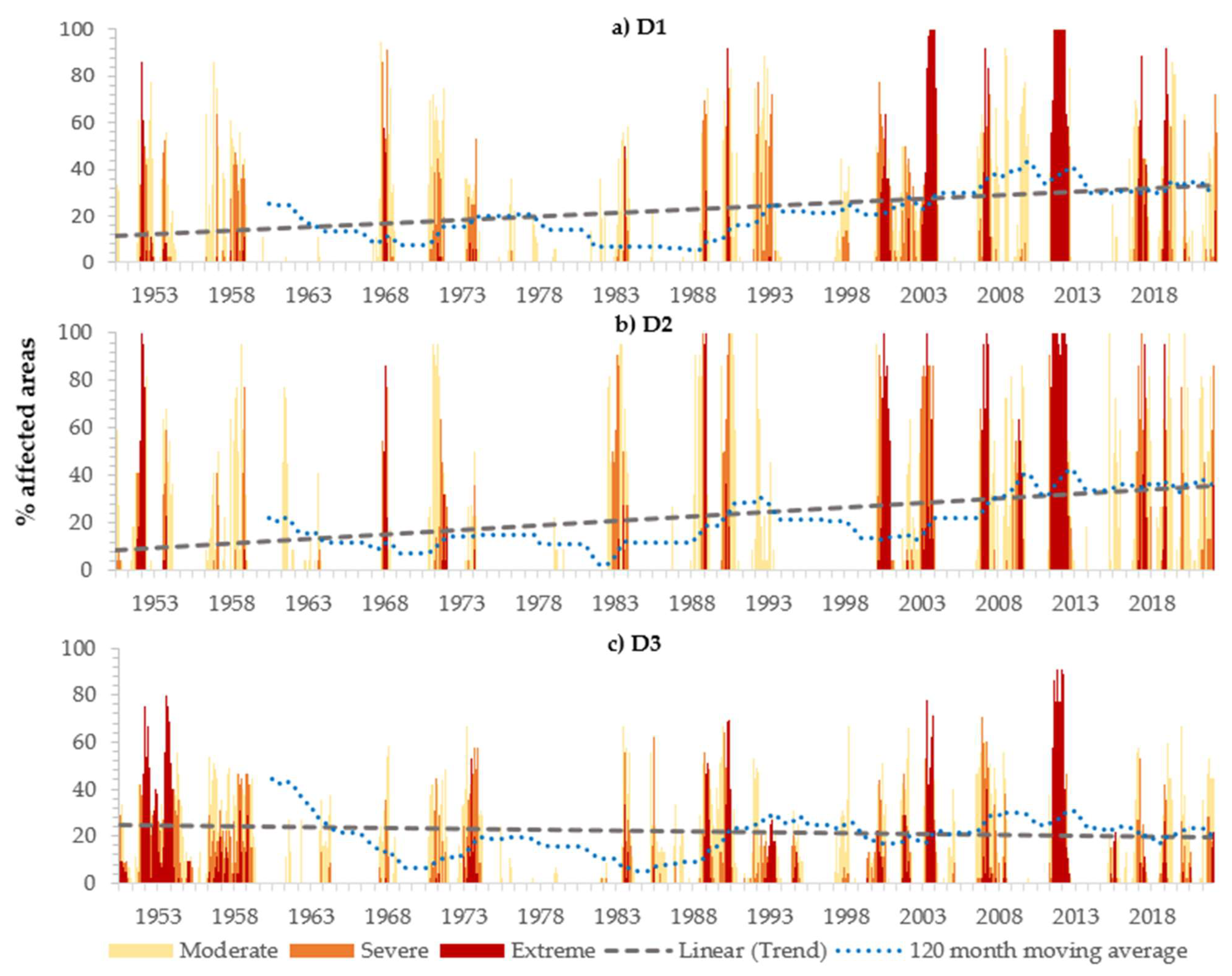
3.2. Temporal Evolution of Drought Areas

The areas affected by drought are an important indicator of the severity of drought events and can also indicate the frequency of various categories of drought. For that purpose, the percentages of area affected by moderate, severe, and extreme drought, according to the SPEI categories of Table 1, were computed for the SPEI6 and SPEI12 series in the three Croatian regions (Figure 6 and Figure 7). The area of each grid center point was accumulated to calculate the total area inside each region D1, D2, and D3, attributed to a specified drought category with SPEI6 and SPEI12 values within those limits. To further understand the linear and nonlinear temporal evolution of the total areas under drought, linear trend lines, along with a moving average considering a running length of 120 months, i.e., 10 years expressing the percent change in drought area, were fitted.

In general terms, it can be seen that, for both SPEI6 (Figure 6) and SPEI12 (Figure 7) fields in each of the regions (D1 to D3), the evolution of the percentage of drought-affected areas shows similar trends, and that, from the year 2000 onwards, the frequency of occurrences of extreme droughts, with an evidently affected cumulative area, increased comparatively to the rest of the time period in both SPEI time-scales. Indeed, droughts are equally spread among each Croatian region and the analysed time window, so that the period with the smallest areas that were affected by drought being the years 1975–1983, with mainly moderate droughts. For SPEI6 and for the entire period from 1950 to 2022, the number of months when drought affected more than 50% of the total area in each region was 180, 192, and 171, respectively, for the central north region (D1), eastern region (D2), and southern region (D3), and 189, 176, and 183 for the respective regions and period in SPEI12. The extraordinary documented drought in Croatia that took place in 2011/2012 [50] is clearly seen in each of the time-scales, especially in SPEI12, where the regions D1 and D2 and almost all the area of D3 experienced an extreme drought situation. Another major drought event occurred in 1950/1951 and 2005/2006 for SPEI6, with 100% of the country experiencing an extreme drought. In the years 1951/1952 and 2005/2006, the SPEI12 droughts affected almost all the regions: D1, D2 and D3.

The change in the percentage of total drought-affected area at both time-scales presents similar linear trends, showing an increasing trend with time in regions D1 and D2, while for region D3, a flattening trend can be seen for SPEI6 and a slightly decreasing trend for SPEI12 (Figure 6 and Figure 7, respectively).

3.3. Changes in Yearly Drought Occurrence Rate

In order to analyse the changes in the yearly drought occurrence rate, the KORE estimator was applied in each of the three regions, from D1 to D3, to the regionalized SPEI series represented by the factor scores that were previously obtained by the PCA. The results, shown in Figure 8 and Figure 9 for SPEI6 and SPEI12, respectively, refer to the occurrences of moderate, severe and extreme droughts, which means that SPEI values were between the drought thresholds (DT) of −0.84 and −1.28, between −1.28 and −1.65, and lower than −1.65, respectively. The dates of the periods under drought conditions are identified by vertical black ticks on the x-axes. A 95% bootstrap confidence band was assigned to each λ(t) curve.

The bandwidth h that appears in Equation (2) was obtained using Silverman’s ‘rule of thumb’ [51], which resulted in values ranging from ca. 30 to 110 months.

Comparison of the results of Figure 8 and Figure 9 for the same drought threshold (DT) shows that the general temporal behaviour of the moderate, severe and extreme drought occurrence rates is relatively independent of the SPEI time-scale (6 or 12 months). For SPEI12 in region D1 (central north region) there is a strong general increase in the occurrence of moderate droughts starting in the 1990s, followed by a decrease that was initiated in around 2010 and lasted until the end of the analysed period, with similar behaviour for severe and extreme droughts. For SPEI6, the same fluctuation pattern in the rate of occurrences of drought is seen but is much less pronounced, as the severe drought category (DT = −1.28) is achieved after the highest rate of annual droughts occurred in 2010; there was only a slight decrease towards the end of the analysed period.

For region D2 (eastern region), the same general increase pattern in the drought occurrence rate was seen among all the drought thresholds and both SPEI time-scales, shown in Figure 7 and Figure 8. Starting at around the beginning of the 1980s for SPEI6 and the 1970s for SPEI12, a persistent increase in the yearly drought occurrence rate is clear, especially for moderate droughts (DT = −0.84), where the increase rate is more pronounced. Region D3 (southern region) has a different pattern, with a general decrease in the drought frequency identified towards the present for both SPEI6 and SPEI12; although this was much less evident, a slight general decrease over time can be seen for extreme drought (DT = −1.65), whereas, for moderate and severe droughts, an increase in the occurrence of drought started around 1975 and reached a peak in 1990, before immediately starting to decrease again until the end of the analysed period.

The obtained results show that the areas most prone to drought occurrence in Croatia, where an upward trend in the number of droughts per year can be seen since 1950, are regions D1 and D2 in both SPEI time-scales. The southern coastal region (D3), with decreasing rates of drought occurrences, showed a different pattern over the entire of the observed period, showing some progressive weakening in droughts (Figure 8 and Figure 9).

3.4. Temporal Trend Analysis

The temporal variability of droughts from 1950 to 2022 was analysed by exploring significant trends, which could be either positive or negative, in the SPEI6 and SPEI12 time series fields with the modified Mann–Kendall test (MMK) [22]. Figure 10 shows the drought trends in the different homogenous regions using Sen’s slope and the results of the MMK test. The color scale represents the magnitude of the slope, and the black dots represents the statistically significant trend at the 0.05 significance level (p < 0.05).

From the results, an overall upward trend (blueish) in D3 is clear, suggesting progressively reduced drought susceptibility over the study period, strictly following the relief of the southern region (D3), which is consistent with the downward trend in the number of drought occurrences shown in Figure 8 and Figure 9 at both time-scales, especially SPEI12. Only a few grid center points show statistically significant upward trends: 3 for SPEI6 and 9 for SPEI12, respectively, in Figure 10a,b. The region of Istria and some coastal parts of Zadar and Sibenik-Knin are the exceptions to the upward trends of D3, with some reddish areas experiencing downward trends for both SPEI time-scales; however, only one of them showed statistical significance (Zadar for SPEI12).

In both the central north region (D1) and eastern region (D2), an opposite general downward trend (reddish), showing more susceptibility to droughts along the study period, was obtained, denoting an intensification of the drought phenomena. This is more pronounced for SPEI12 due to the higher trend slope (a more reddish area) and a slightly higher number of grid center points with statistically significant trends. In fact, almost all the trends identified in regions D1 and D2 have statistical significance, with marked grid center points covering most of the regions (black dots). These results are somehow in agreement with those of Figure 8 and Figure 9 in terms of the frequency of different categories of drought occurrences showing an upward trend for both SPEI timescales, except for Figure 9 in region D1, which is not as clear.

4. Discussion

According to the Seventh National Communication of the Republic of Croatia under the UNFCCC (2018) and Strategy on Adaptation to Climate Change in Croatia (2020) [52,53], several priorities are highlighted. One of them is strengthening the professional, scientific and management capacities to deal with the risks of climate change’s impact on water resources. The proposed measures and activities include the development of monitoring systems, data acquisition and research as fundamental for the estimation of vulnerabilities in the agricultural and environmental sectors. Within this framework, the obtained regionalization, by dividing mainland Croatia into three distinct homogenous regions, will certainly provide new prospects and help in future activities, and is especially relevant tp the most susceptible areas of Croatia.

Recent investigations of extreme hydrological events were mostly focused on observed changes in the seasonal and annual air temperature and precipitation amounts in Croatia [26], or studying the spatiotemporal characteristics of the mean and maximum dry spells in Croatia [54], but they did not deal with drought as a complex hydro-climatological event that is inter-related with many of the morphoclimatic characteristics of a certain area.

Research involving drought phenomena in Croatia, and its severity in terms of duration and intensity, was mostly conducted at regional or local scales [20,21,22], or focused on specific drought events such as a meteorological analysis of an extreme drought in 2011/2012, which seriously affected the territory of Croatia [50]. In this research, the spatial and temporal characteristics of droughts obtained using the SPEI6 and SPEI12, calculated using the two main climate drivers (precipitation and temperature), seem to be aligned with the geomorphological characteristics of the identified regions. Region D3, which covers the mountain system of the Dinarides and the Adriatic basin, has the highest average elevation in the country and the highest average annual precipitation, while in regions D1 and D2, representing the Pannonian basin, the average annual precipitation progressively decreases towards the eastern areas. The eastern region (D2) covers all the Lowland areas, with elevations up to 200 m, and represents 50% of the total area of the country.

Although these results should be taken with caution due to the complexity of the climate system, they further highlight the need for the development of future drought research and in-depth studies on drought variability and the respective main drivers in the identified regions. Similar results were found in some of the literature examples around the world, such as the work of [8,11,12] or [49], where the identification of homogeneous regions was consistent with the morphological and climate characteristics of those territories, which seems to play an important role in shaping drought areal patterns.

From the results obtained for SPEI6, the time-scale typically associated with agricultural drought occurrence [6], the linear trend and the 120 month moving average in the drought areal evolution of regions D1 and D2 (Figure 6 and Figure 7) are illustrative of the upward trend in areas affected by drought, which is particularly relevant since the Pannonian region (covered by D1 and D2) is the most important and largest agricultural region of Croatia, with highly developed intensive arable farming and high yields of most of the crops [55]. If the drought-affected areas in these regions are affected within the months of May–October, the droughts tend to be more critical, since this is the hottest period of the year in Croatia (Bjelovar and Gradište from Figure 2a) and the atmospheric evaporative demand is higher. In most of region D3, the areal evolution trend is almost negligible and even slightly negative for the SPEI12, a time-scale that can effectively characterize the country’s historical drought annually.

In general terms, for both regions D1 and D2, the number of drought occurrences through KORE is also increasing, showing some oscillatory periods over time, independently of the drought category and SPEI time-scale. For region D3 and both SPEI6 and SPEI12, some evident downward trends are seen, especially for moderate and severe droughts, and a slight decrease in extreme droughts. The MMK trends applied to the SPEI grid center point series seems to have some relation with the drought areal evolution and occurrence rate analysis, since the trend signals are predominantly significant in regions D1 and D2, showing more locations with significant negative trends compared to the few mainly non-significant positive trends that can be seen in region D3. In region D3, for both SPEI time-scales, the results seem to be in accordance with the results of [26] for the period 1960–2020, since for the mountainous system of the Dinarides, the authors identified a significant increase in precipitation due to the occurrence of very wet days using the daily intensity index, while the Imotski station (Southern Adriatic coast) detected a non-significant upward trend in the annual precipitation [56]. However, the effect of temperature on the aggravation of drought conditions seems to be less complex, since several authors show that statistically significant increases in air temperature, especially in the mean annual temperatures, consistently occurred all over the country in the last 50 years [57,58].

5. Conclusions

To better deal with climate change and its impacts, it is crucial, as a first step, to understand climate variability at a sub-regional scale; therefore, a generalized assessment of historical drought behaviour emerges as one of the main priorities when characterizing the existence of water deficits at a subannual and annual scale throughout any country.

The present study accomplishes part of this objective by providing a quite complete insight into the drought phenomena in Croatia with such a spatial resolution. Based on the E-OBS dataset, the SPEI was calculated over 6- and 12-month time-scales for the period from 1950 to 2022. The PCA and K-means methods were used for drought regionalization and to explore the spatial patterns of drought distribution, as well as describing and plotting drought characteristics such as drought occurrence frequency and drought severity by calculating the percentage of drought-affected areas. The drought trends were also analysed using the MMK method coupled with Sen’s slope. The main findings of the study are as follows:

(1)

Based on PCA and K-means validation, Croatia was divided into three homogeneous regions: the central north region (D1), eastern region (D2) and southern region (D3).

(2)

The central north region (D1) and eastern region (D2) showed an upward trend in the percentage of areas affected by drought in the whole study period for both SPEI6 and SPEI12, but in the southern region (D3), a negligible trend was obtained for SPEI6 and a downward trend was seen, meaning that progressively fewer areas affected by drought were obtained for SPEI12. Both the D1 and D2 areas have large amounts of non-irrigated agricultural land and grassland, resulting in high ecological vulnerability.

(3)

Region D1 (the central north region) experienced an increase in the drought occurrence rate from 1950 until around 2010, and some decreases occurred in the last 10 years, which were especially pronounced in SPEI12. The eastern region (D2) experienced a generalized continuous increase in the drought occurrence rate from 1950 to 2022 in all drought categories and at SPEI time-scales. In the southern region (D3), a decrease in the drought occurrence rate was obtained with one interruption peak. According to the nature of the SPEI calculation procedure, an increase in the number of drought occurrences over the years means that there are progressively longer periods of time with negative water balances, which necessarily lead to to bigger challenges in water management practices.

(4)

A generalized change towards increased susceptibility to drought conditions in most areas of D1 and D2 was obtained using the MMK test, with strong statistical significance in both SPEI6 and SPEI12. Given the Sen’s slope values obtained from the trend analysis applied to the SPEI series, more intense drought events are expected in those areas. In the southern region (D3), the trend of less susceptibility to drought conditions spatially follows the mountainous areas of the Dinarides, with less statistical significance. The region of Istria and some coastal parts of Zadar and Sibenik-Knin are the exceptions to the general pattern found in D3, since some localized areas will become a bit more susceptible to drought, which is seen in both SPEI time-scales.

(5)

In general terms, the west (Mediterranean climate) is becoming less susceptible to drought, while the east (continental climate) is becoming more prone to an intensification of drought events, showing a greater increase in the areas affected by drought over the years and an increasing rate of occurrence for annual droughts. Although the Mediterranean region is usually at the center of drought research, it is in the mainly agricultural mainland of Croatia that drought conditions seem to have worsened.

Due to Croatia’s complex morphoclimatic characteristics, there are still some limitations to using the obtained results, such as delving into the underlying causes and implications of the regional spatio-temporal drought patterns found in the homogeneous regions, or how these patterns relate to climate change and other environmental factors, such as soil moisture or vegetation, and their roles in shaping areas of drought susceptibility. Clearer evidence from this study suggests that, in addition to climate drivers, topographical features greatly influence the spatial patterns that are identified here. However, the spatio-temporal variability of the identified droughts given the limitations of using only SPEI6 and SPEI12, suggests that other time-scales should be considered in future studies in order to obtain more information on the drought behaviour in each homogenous region.

To build on the presented results, future studies should also investigate the main teleconnection patterns that could explain drought variability in the country; since temperature plays an important role on drought conditions, the effect of considering more physically realistic PET methods in drought characterization, such as the FAO-56 Penman-Monteith [58], should also be considered.

To reduce and mitigate drought impacts, the development and implementation of risk-based drought management plans is encouraged to support policy-makers and water resources managers in developing the best strategies. The authors hope that the achieved results could provide valuable supporting information by highlighting regions that are more susceptible to drought than others, where the severity, number of yearly occurrences and affected areas have been increasing over the years.

References

1. Dadson, S.; Penning-Rowsell, E.; Garrick, D.; Hope, R.; Hall, J.; Hughes, J. Water Science, Policy, and Management: A Global Challenge; Wiley Blackwell: Hoboken, NJ, USA; Chichester, UK, 2020; ISBN 978-1-119-52060-3. [Google Scholar]
2. United Nations Convention to Combat Desertification (UNCCD). Drought in Numbers 2022-Restoration for Readiness and Resilience; United Nations: Abidjan, Côte d’Ivoire, 2022.
3. World Meteorological Organization (WMO). Drought and Water Scarcity (WMO-No. 1284); World Climate Programme (WCP): Geneve, Switzerland, 2022. [Google Scholar]
4. Van Loon, A.F.; Van Lanen, H.A.J. Making the Distinction between Water Scarcity and Drought Using an Observation-Modeling Framework: Distinguishing between Water Scarcity and Drought. Water Resour. Res. 2013, 49, 1483–1502. [Google Scholar] [CrossRef]
5. McKee, T.B.; Doesken, N.J.; Kleist, J. The Relationship of Drought Frequency and Duration to Time Scales. Eighth Conference on Applied Climatology, Anaheim, CA, USA, 17–22 January 1993; 17, pp. 179–183. [Google Scholar]
6. Vicente-Serrano, S.M.; Beguería, S.; López-Moreno, J.I. A Multiscalar Drought Index Sensitive to Global Warming: The Standardized Precipitation Evapotranspiration Index. J. Clim. 2010, 23, 1696–1718. [Google Scholar] [CrossRef]
7. Vicente-Serrano, S.M. Spatial and Temporal Analysis of Droughts in the Iberian Peninsula (1910–2000). Hydrol. Sci. J. 2006, 51, 83–97. [Google Scholar] [CrossRef]
8. Santos, J.F.; Pulido-Calvo, I.; Portela, M.M. Spatial and Temporal Variability of Droughts in Portugal. Water Resour. Res. 2010, 46. [Google Scholar] [CrossRef]
9. Raziei, T.; Martins, D.S.; Bordi, I.; Santos, J.F.; Portela, M.M.; Pereira, L.S.; Sutera, A. SPI Modes of Drought Spatial and Temporal Variability in Portugal: Comparing Observations, PT02 and GPCC Gridded Datasets. Water Resour. Manag. 2015, 29, 487–504. [Google Scholar] [CrossRef]
10. Espinosa, L.A.; Portela, M.M. Grid-Point Rainfall Trends, Teleconnection Patterns, and Regionalised Droughts in Portugal (1919–2019). Water 2022, 14, 1863. [Google Scholar] [CrossRef]
11. Di Nunno, F.; Granata, F. Spatio-Temporal Analysis of Drought in Southern Italy: A Combined Clustering-Forecasting Approach Based on SPEI Index and Artificial Intelligence Algorithms. Stoch. Environ. Res. Risk Assess. 2023, 37, 2349–2375. [Google Scholar] [CrossRef]
12. Xie, P.; Lei, X.; Zhang, Y.; Wang, M.; Han, I.; Chen, Q. Cluster Analysis of Drought Variation and Its Mutation Characteristics in Xinjiang Province, during 1961–2015. Hydrol. Res. 2018, 49, 1016–1027. [Google Scholar] [CrossRef]
13. Araneda-Cabrera, R.J.; Bermudez, M.; Puertas, J. Revealing the Spatio-Temporal Characteristics of Drought in Mozambique and Their Relationship with Large-Scale Climate Variability. J. Hydrol. Reg. Stud. 2021, 38, 100938. [Google Scholar] [CrossRef]
14. Spinoni, J.; Naumann, G.; Vogt, J.; Barbosa, P. European Drought Climatologies and Trends Based on a Multi-Indicator Approach. Glob. Planet. Change 2015, 127, 50–57. [Google Scholar] [CrossRef]
15. Blauhut, V.; Stoelzle, M.; Ahopelto, L.; Brunner, M.I.; Teutschbein, C.; Wendt, D.E.; Akstinas, V.; Bakke, S.J.; Barker, L.J.; Bartošová, L.; et al. Lessons from the 2018–2019 European droughts: A collective need for unifying drought risk management. Nat. Hazards Earth Syst. Sci. 2022, 22, 2201–2217. [Google Scholar] [CrossRef]
16. Barron, E.; van Manen, H. The World Climate and Security Report 2022: Climate Security Snapshot-The Balkans; Product of the Expert Group of the International Military Council on Climate and Security; An institute of the Council on Strategic Risks; Center for Climate and Security: The Hague, The Netherlands, 2022. [Google Scholar]
17. Knez, S.; Štrbac, S.; Podbregar, I. Climate Change in the Western Balkans and EU Green Deal: Status, Mitigation and Challenges. Energy Sustain. Soc. 2022, 12, 1. [Google Scholar] [CrossRef]
18. Juraj, J.; Tadić, L.; Brleković, T.; Potočki, K.; Leko-Kos, M. Application of Principal Component Analysis to Drought Indicators of Three Representative Croatian Regions. Elektron. Časopis Građev. Fak. Osijek 2021, 12, 41–55. [Google Scholar] [CrossRef]
19. Brleković, T.; Tadić, L. Hydrological Drought Assessment in a Small Lowland Catchment in Croatia. Hydrology 2022, 9, 79. [Google Scholar] [CrossRef]
20. Pandžić, K.; Likso, T.; Curić, O.; Mesić, M.; Pejić, I.; Pasarić, Z. Drought Indices for the Zagreb-Grič Observatory with an Overview of Drought Damage in Agriculture in Croatia. Theor. Appl. Climatol. 2020, 142, 555–567. [Google Scholar] [CrossRef]
21. Revelle, W. An Introduction to Psychometric Theory with Applications in R, 2023rd ed.; Springer International Publishing: Berlin/Heidelberg, Germany, 2023. [Google Scholar]
22. Hamed, K.H.; Ramachandra Rao, A. A Modified Mann-Kendall Trend Test for Autocorrelated Data. J. Hydrol. 1998, 204, 182–196. [Google Scholar] [CrossRef]
23. Perčec Tadić, M.; Pasarić, Z.; Guijarro, J.A. Croatian High-Resolution Monthly Gridded Dataset of Homogenised Surface Air Temperature. Theor. Appl. Climatol. 2023, 151, 227–251. [Google Scholar] [CrossRef]
24. Gajić-Čapka, M.; Cindrić, K.; Pasarić, Z. Trends in Precipitation Indices in Croatia, 1961–2010. Theor. Appl. Climatol. 2015, 121, 167–177. [Google Scholar] [CrossRef]
25. Perčec Tadić, M.; Gajić-Čapka, M.; Zaninović, K.; Cindric, K. Drought Vulnerability in Croatia. Agric. Conspec. Sci. 2014, 79, 31–38. [Google Scholar]
26. Cindric Kalin, K.; Patalen, L.; Marinovic, I.; Pasaric, Z. Trends in Temperature and Precipitation Indices in Croatia, 1961–2020. In Proceedings of the Copernicus Meetings, EMS Annual Meeting 2022, Bonn, Germany, 5–9 September 2022. [Google Scholar]
27. Cornes, R.C.; Van Der Schrier, G.; Van Den Besselaar, E.J.M.; Jones, P.D. An Ensemble Version of the E-OBS Temperature and Precipitation Data Sets. J. Geophys. Res. Atmos. 2018, 123, 9391–9409. [Google Scholar] [CrossRef]
28. Thornthwaite, C.W. An Approach toward a Rational Classification of Climate. Geogr. Rev. 1948, 38, 55. [Google Scholar] [CrossRef]
29. Alam, N.M.; Sharma, G.C.; Moreira, E.; Jana, C.; Mishra, P.K.; Sharma, N.K.; Mandal, D. Evaluation of Drought Using SPEI Drought Class Transitions and Log-Linear Models for Different Agro-Ecological Regions of India. Phys. Chem. Earth Parts ABC 2017, 100, 31–43. [Google Scholar] [CrossRef]
30. Dikshit, A.; Pradhan, B.; Huete, A. An Improved SPEI Drought Forecasting Approach Using the Long Short-Term Memory Neural Network. J. Environ. Manag. 2021, 283, 111979. [Google Scholar] [CrossRef] [PubMed]
31. Svoboda, M.D.; Fuchs, B.A. Handbook of Drought Indicators and Indices; World Meteorological Organization: Geneva, Switzerland, 2016; ISBN 978-92-63-11173-9. [Google Scholar]
32. Liu, C.; Yang, C.; Yang, Q.; Wang, J. Spatiotemporal Drought Analysis by the Standardized Precipitation Index (SPI) and Standardized Precipitation Evapotranspiration Index (SPEI) in Sichuan Province, China. Sci. Rep. 2021, 11, 1280. [Google Scholar] [CrossRef]
33. Agnew, C. Using the SPI to Identify Drought. Drought Network News, May 2000; 12p. [Google Scholar]
34. López-Moreno, J.I.; Vicente-Serrano, S.M.; Zabalza, J.; Beguería, S.; Lorenzo-Lacruz, J.; Azorin-Molina, C.; Morán-Tejeda, E. Hydrological Response to Climate Variability at Different Time Scales: A Study in the Ebro Basin. J. Hydrol. 2013, 477, 175–188. [Google Scholar] [CrossRef]
35. Bonaccorso, B.; Bordi, I.; Cancelliere, A.; Rossi, G.; Sutera, A. Spatial Variability of Drought: An Analysis of the SPI in Sicily. Water Resour. Manag. 2003, 17, 273–296. [Google Scholar] [CrossRef]
36. Smith, L.I. A Tutorial on Principal Components Analysis; Cornell University: Ithaca, NY, USA, 2002. [Google Scholar]
37. Hair, J.F. Multivariate Data Analysis, 6th ed.; Pearson Prentice Hall: Upper Saddle River, NJ, USA, 2006; ISBN 978-0-13-032929-5. [Google Scholar]
38. Woods, C.M.; Edwards, M.C. Essential Statistical Methods for Medical Statistics; Rao, C.R., Miller, J.P., Rao, D.C.R., Eds.; Elsevier: Amsterdam, The Netherlands, 2011; ISBN 978-0-444-53737-9. [Google Scholar]
39. Vicente-Serrano, S.; González-Hidalgo, J.; De Luis, M.; Raventós, J. Drought Patterns in the Mediterranean Area: The Valencia Region (Eastern Spain). Clim. Res. 2004, 26, 5–15. [Google Scholar] [CrossRef]
40. Kahya, E.; Kalaycı, S.; Piechota, T.C. Streamflow Regionalization: Case Study of Turkey. J. Hydrol. Eng. 2008, 13, 205–214. [Google Scholar] [CrossRef]
41. Shukla, S.; Mostaghimi, S.; Petrauskas, B.; Al-Smadi, M. Multivariate Technique for Baseflow Separation Using Water Quality Data. J. Hydrol. Eng. 2000, 5, 172–179. [Google Scholar] [CrossRef]
42. Mudelsee, M.; Börngen, M.; Tetzlaff, G.; Grünewald, U. No Upward Trends in the Occurrence of Extreme Floods in Central Europe. Nature 2003, 425, 166–169. [Google Scholar] [CrossRef]
43. Silva, A.T.; Portela, M.M.; Naghettini, M. Nonstationarities in the Occurrence Rates of Flood Events in Portuguese Watersheds. Hydrol. Earth Syst. Sci. 2012, 16, 241–254. [Google Scholar] [CrossRef]
44. Portela, M.M.; Dos Santos, J.F.; Silva, A.T.; Benitez, J.B.; Frank, C.; Reichert, J.M. Drought Analysis in Southern Paraguay, Brazil and Northern Argentina: Regionalization, Occurrence Rate and Rainfall Thresholds. Hydrol. Res. 2015, 46, 792–810. [Google Scholar] [CrossRef]
45. Portela, M.M.; Santos, J.F.; Purcz, P.; Silva, A.T.; Hlavatá, H. A Comprehensive Drought Analysis in Slovakia Using SPI. Eur. Water 2015, 51, 15–31. [Google Scholar]
46. Diggle, P. A Kernel Method for Smoothing Point Process Data. Appl. Stat. 1985, 34, 138. [Google Scholar] [CrossRef]
47. Sen, P.K. Estimates of the Regression Coefficient Based on Kendall’s Tau. J. Am. Stat. Assoc. 1968, 63, 1379–1389. [Google Scholar] [CrossRef]
48. Mann, H.B. Nonparametric Tests Against Trend. Econometrica 1945, 13, 245. [Google Scholar] [CrossRef]
49. Kamruzzaman, M.; Almazroui, M.; Salam, M.A.; Mondol, M.A.H.; Rahman, M.M.; Deb, L.; Kundu, P.K.; Zaman, M.A.U.; Islam, A.R.M.T. Spatiotemporal Drought Analysis in Bangladesh Using the Standardized Precipitation Index (SPI) and Standardized Precipitation Evapotranspiration Index (SPEI). Sci. Rep. 2022, 12, 20694. [Google Scholar] [CrossRef]
50. Cindrić, K.; Telišman Prtenjak, M.; Herceg-Bulić, I.; Mihajlović, D.; Pasarić, Z. Analysis of the Extraordinary 2011/2012 Drought in Croatia. Theor. Appl. Climatol. 2016, 123, 503–522. [Google Scholar] [CrossRef]
51. Silverman, B.W. Density Estimation for Statistics and Data Analysis, 1st ed.; Routledge: London, UK, 2018; ISBN 978-1-315-14091-9. [Google Scholar]
52. Climate change adaptation strategy in the Republic of Croatia for the period up to 2040 with a view to 2070. Official Gazette of the Republic of Croatia 46/2020. Available online: https://faolex.fao.org/docs/pdf/cro207819.pdf (accessed on 11 June 2023).
53. Seventh National Communication of the Republic of Croatia under the United Nation Framework Convention on the Climate Change (UNFCCC). 2018. Available online: https://unfccc.int/sites/default/files/resource/IDR7_HRV_complete.pdf (accessed on 20 May 2023).
54. Cindrić Kalin, K.; Pasarić, Z. Regional Patterns of Dry Spell Durations in Croatia. Int. J. Climatol. 2022, 42, 5503–5519. [Google Scholar] [CrossRef]
55. Agricultural Regions of Croatia. The Soils of Croatia; World Soils Book Series; Springer: Dordrecht, The Netherlands, 2013; pp. 23–36. ISBN 978-94-007-5814-8. [Google Scholar]
56. Vrsalović, A.; Andrić, I.; Bonacci, O.; Kovčić, O. Climate Variability and Trends in Imotski, Croatia: An Analysis of Temperature and Precipitation. Atmosphere 2023, 14, 861. [Google Scholar] [CrossRef]
57. Roushangar, K.; Ghasempour, R. Multi-Temporal Analysis for Drought Classifying Based on SPEI Gridded Data and Hybrid Maximal Overlap Discrete Wavelet Transform. Int. J. Environ. Sci. Technol. 2022, 19, 3219–3232. [Google Scholar] [CrossRef]
58. Allen, R.G.; Pereira, L.S.; Raes, D.; Smith, M. Crop Evapotranspiration: Guidelines for Computing Crop Water Requirements; Food and Agriculture Organization of the United Nations, Ed.; FAO Irrigation and Drainage Paper; Food and Agriculture Organization of the United Nations: Rome, Italy, 1998; ISBN 978-92-5-104219-9. [Google Scholar]
Figure 1. (a) General location of Croatia and its hypsometric map, with grey marks that illustrate the E-OBS grid center points (0.25° resolution). Annual series of (b) precipitation and (c) mean temperature (solid lines), with positive (blue bars) and negative (red bars) anomalies in respect to the mean from 1950 to 2021, trend lines (dotted lines) indicate linear tendencies.
Water 15 03806 g001
Figure 2. Boxplots of mean monthly temperatures (a) and monthly precipitation (b) time series (1981–2022) between selected meteorological stations (identified by title name) and the respective nearest grid center points from E-OBS.
Water 15 03806 g002aWater 15 03806 g002b
Figure 3. Scree plots of the Eigenvalues and percentage of variance explained for the first 10 PCs at the SPEI6 (a) and SPEI12 (b).
Water 15 03806 g003
Figure 4. Spatial distribution of the factor loadings for SPEI6 and SPEI12. Top, SPEI6: (a) RPC D1 (central north region); (b) RPC D2 (eastern region); (c) RPC D3 (southern region). Bottom, SPEI12: (d) RPC D1 (central north region); (e) RPC D2 (eastern region); (f) RPC D3 (southern region). Solid lines (in black) indicate the contour line for a significant correlation of r = 0.6.
Water 15 03806 g004
Figure 5. Test comparison of clusters analysis with two, three, and four classification groups. On the top, from (ac), for SPEI6, and on the bottom, from (df), for SPEI12.
Water 15 03806 g005
Figure 6. Temporal evolution of the percentage of area affected by Moderate (yellow), Severe (orange) and Extreme (red) drought categories for SPEI6 series in each of the homogeneous regions of (a) D1, (b) D2 and (c) D3 (in correspondence with Figure 4a–c)).
Water 15 03806 g006
Figure 7. Temporal evolution of the percentage of area affected by Moderate (yellow), Severe (orange) and Extreme (red) drought categories for SPEI12 series in each of the homogeneous regions of (a) D1, (b) D2 and (c) D3 (in correspondence with Figure 4d–f)).
Water 15 03806 g007
Figure 8. Regionalized SPEI6 from 1950 to 2022. Time-dependent occurrence rates of drought periods in homogeneous regions (a) D1, (b) D2, and (c) D3, as shown in Figure 4a–c, respectively. Left y-axis: the regionalized SPEI6 in dark blue. Right y-axis: the number of months under drought conditions per year, λ(t), categorized as moderate (in yellow), severe (in orange), and extreme (in red); the confidence band is represented by the grey area around λ(t). Horizontal dashed lines, distinct from zero, indicate the thresholds (DT) adopted for different types of drought conditions. Vertical ticks mark the dates of periods under drought conditions.
Water 15 03806 g008
Figure 9. Regionalized SPEI12 from 1950 to 2022. Time-dependent occurrence rates of drought periods in homogeneous regions (a) D1, (b) D2, and (c) D3 as illustrated in Figure 4d–f), respectively. Left y-axis: the regionalized SPEI12 in dark blue. Right y-axis: the number of months under drought conditions per year, λ(t), categorized as moderate (in yellow), severe (in orange), and extreme (in red); the confidence band is represented by the grey area around λ(t). Horizontal dashed lines, distinct from zero, indicate the thresholds (DT) adopted for different types of drought conditions. Vertical ticks mark the dates of periods under drought conditions.
Water 15 03806 g009
Figure 10. Drought trends for SPEI6 (a) and SPEI12 (b) based on the modified Mann–Kendall test. The black dots represent the statistically significant trends at the 0.05 significance level.
Water 15 03806 g010