
Monthly Runoff Prediction by Combined Models Based on Secondary Decomposition at the Wulong Hydrological Station in the Yangtze River Basin


Abstract
:1. Introduction
2. Materials and Methods
2.1. Decomposition–Prediction Model
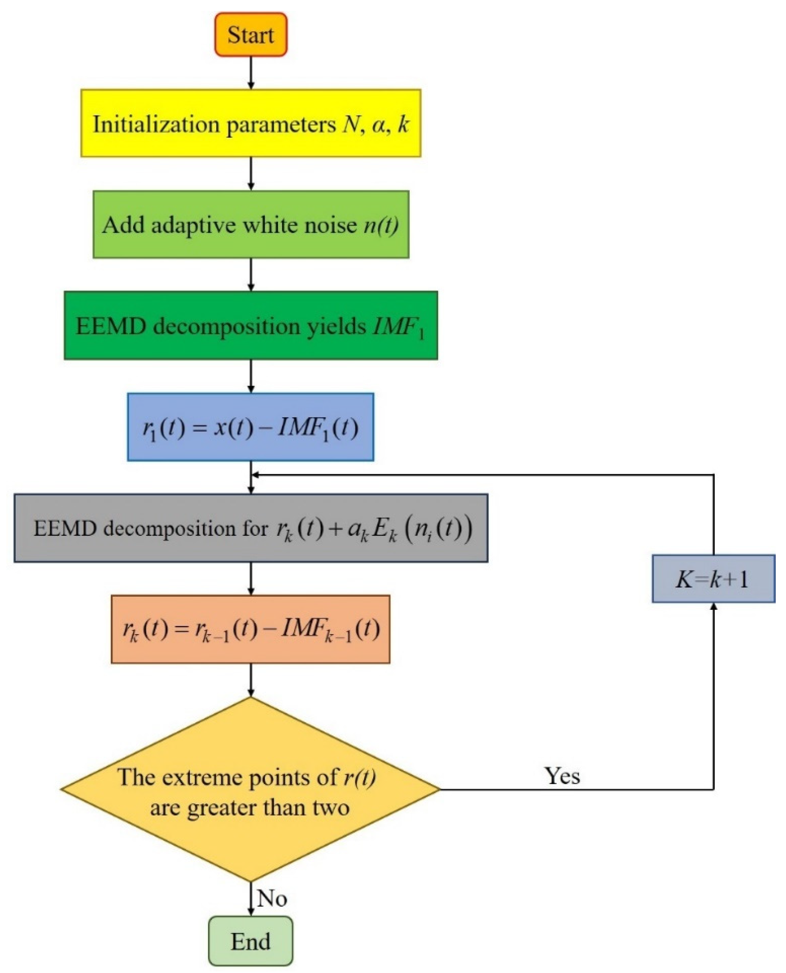
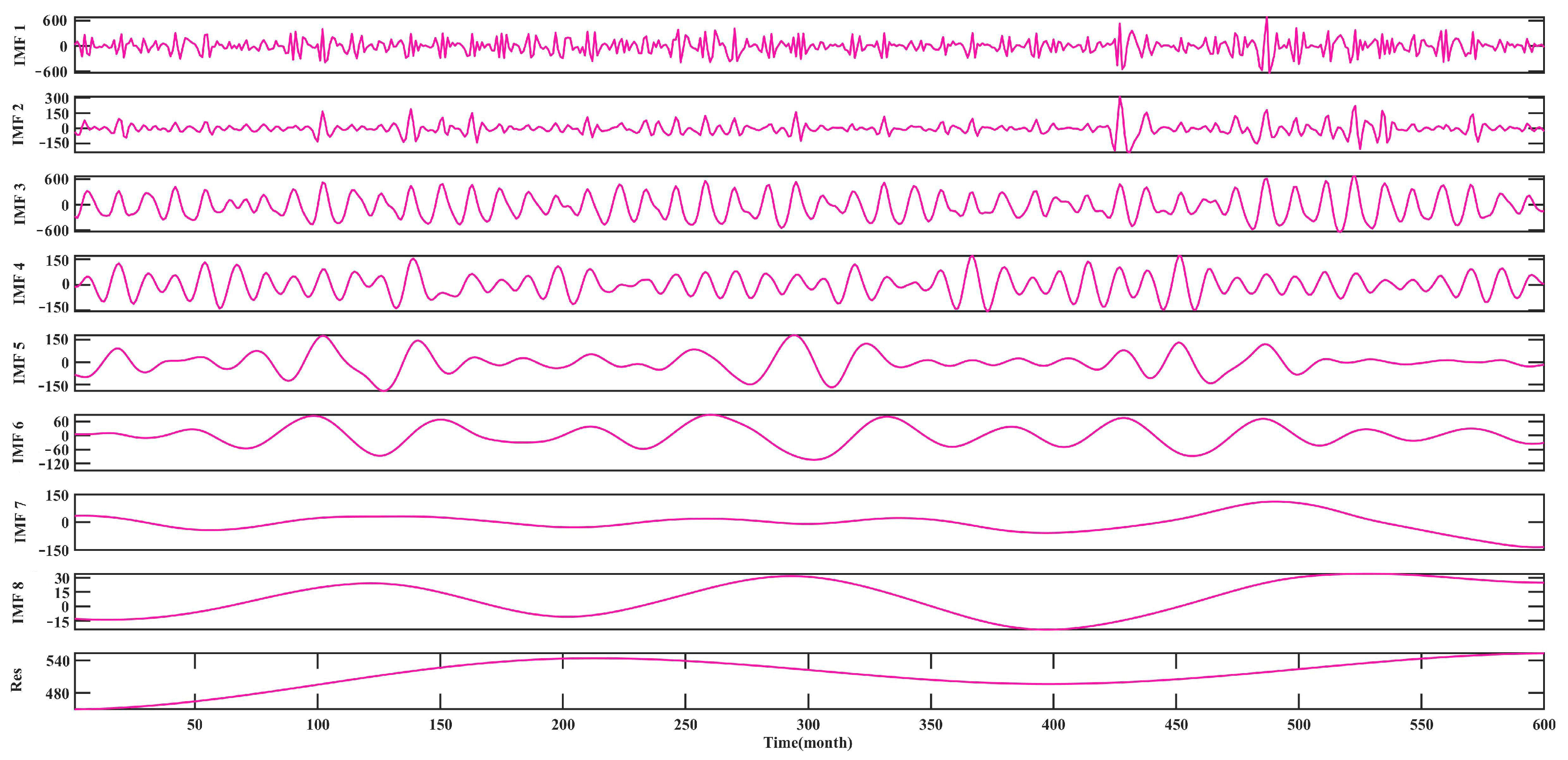
2.1.1. CEEMDAN
- (1)
- The signal , with the addition of adaptive white noise , is decomposed using the EMD algorithm to obtain the first IMF component:
- (2)
- The first residual component signal is calculated:
- (3)
- are the k IMF components generated by EMD decomposition, and is decomposed until the first IMF component is decomposed, then the second IMF component is calculated:
- (4)
- Repeat step (3) to obtain the k-th and the residual component :
- (5)
- Continue to perform step (4) until the residual signal cannot be decomposed further; that is, there are no more than two extreme points of the residual signal. At the end of the algorithm, there are K inherent modes, and the final residual signal is:
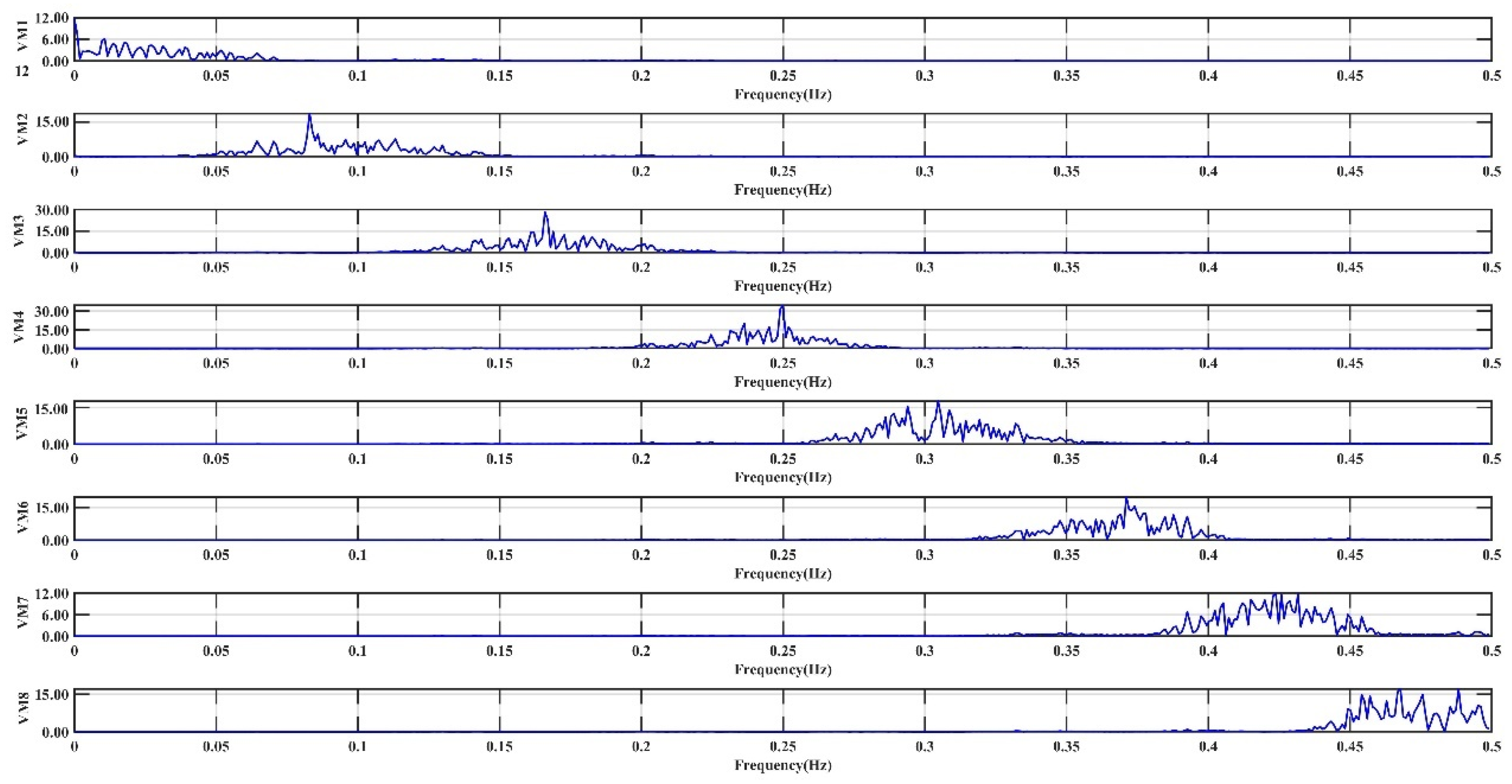
2.1.2. VMD
- (1)
- Using the central frequency observation method to determine the number of variational modes (VMs) extracted by VMD, let . Employ VMD for a secondary decomposition of IMF1. When , the center frequencies of the VMD-extracted modes are close to 0, then is the final selected number of modes.
- (2)
- For the highest frequency component within the IMF components, the Hilbert transform is applied to obtain the analytical signal of the original mode, which yields the one-sided spectrum.where is the unit pulse function; j represents an imaginary unit; is the r-th mode; and represents convolution.
- (3)
- Shift the spectrum of each mode to the baseband by adjusting the estimated center frequencies of the entire using the multiplication of by , bringing all the modes to the fundamental frequency band.
- (4)
- Utilize the constrained variational model to determine the bandwidth of each mode component.where is the angular frequency of each mode; is the highest frequency component to be decomposed twice; and means to take the partial derivative of t.
- (5)
- By introducing the quadratic penalty factor and the Lagrange multiplier operator , the optimal solution of the constrained variational model can be obtained, resulting in the optimal mode. The quadratic penalty factor ensures signal reconstruction accuracy, while the Lagrange multiplier operator reinforces the constraints.
2.1.3. LSTM
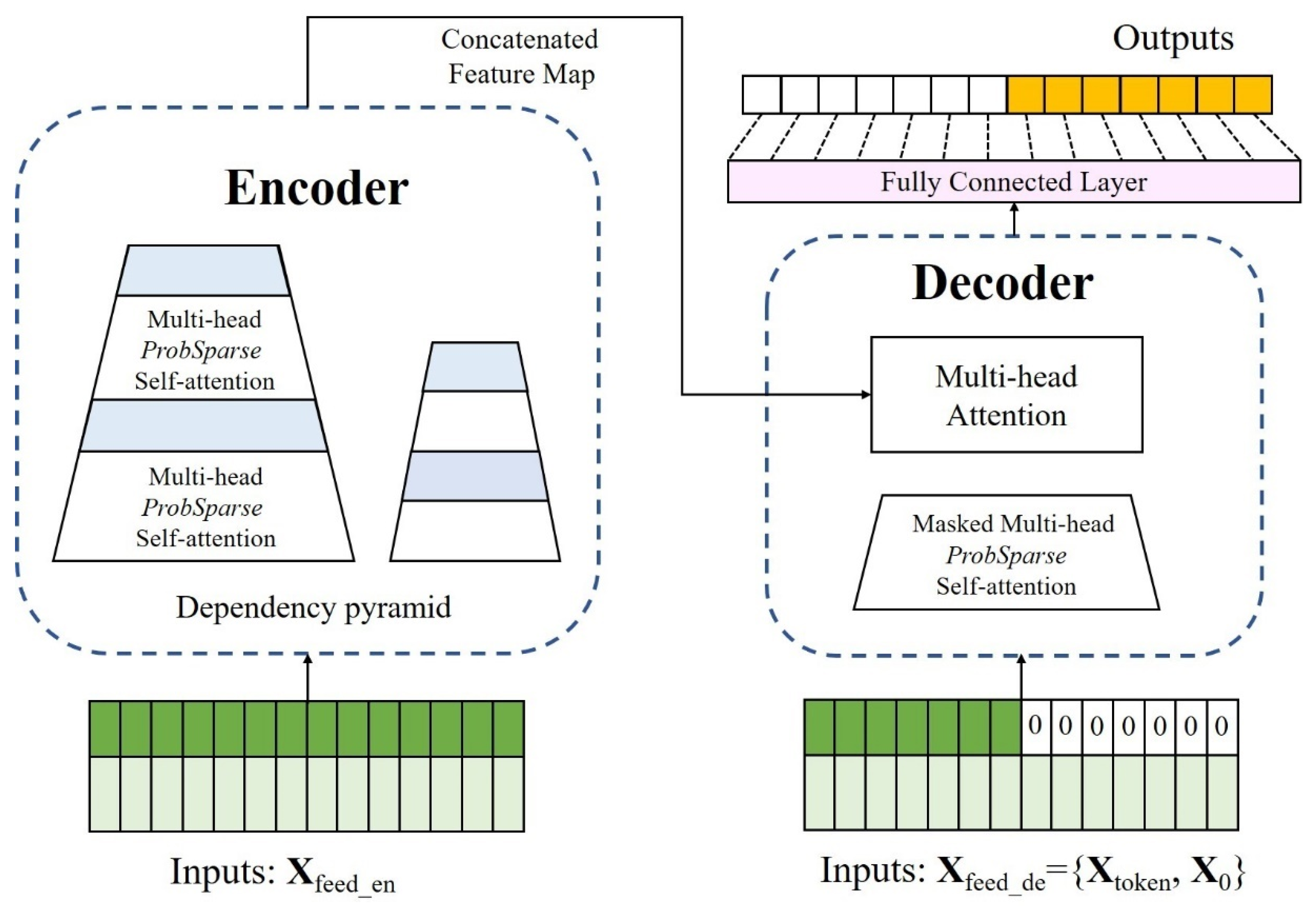
2.1.4. Informer
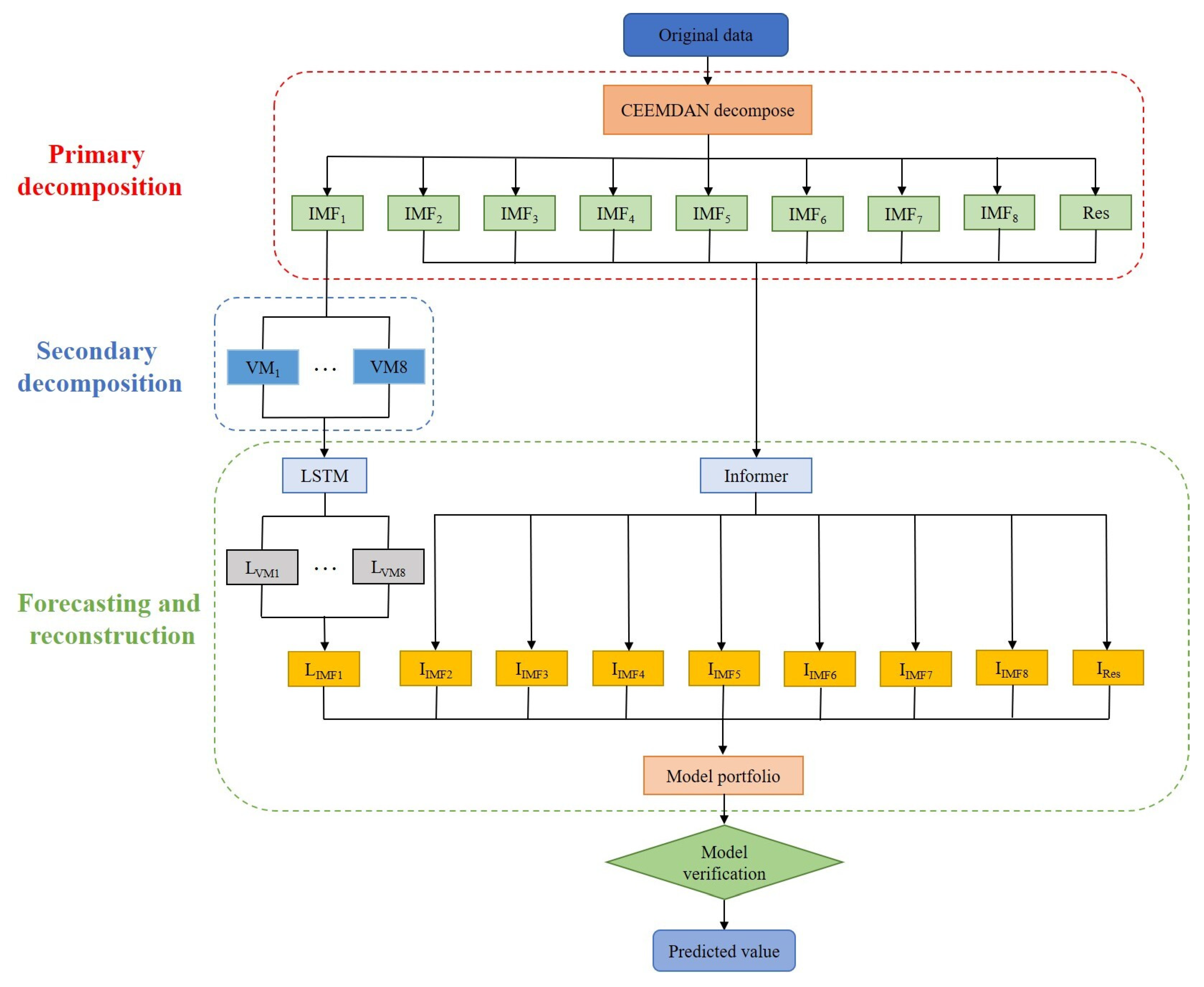
2.2. CEEMDAN-VMD-LSTM-Informer Coupled Model
2.3. Parameter Setting
2.4. Seasonal Exponential Smoothing Model
2.5. Evaluation Indicators
3. Case Study
3.1. Study Area
3.2. Runoff Characteristics Analysis
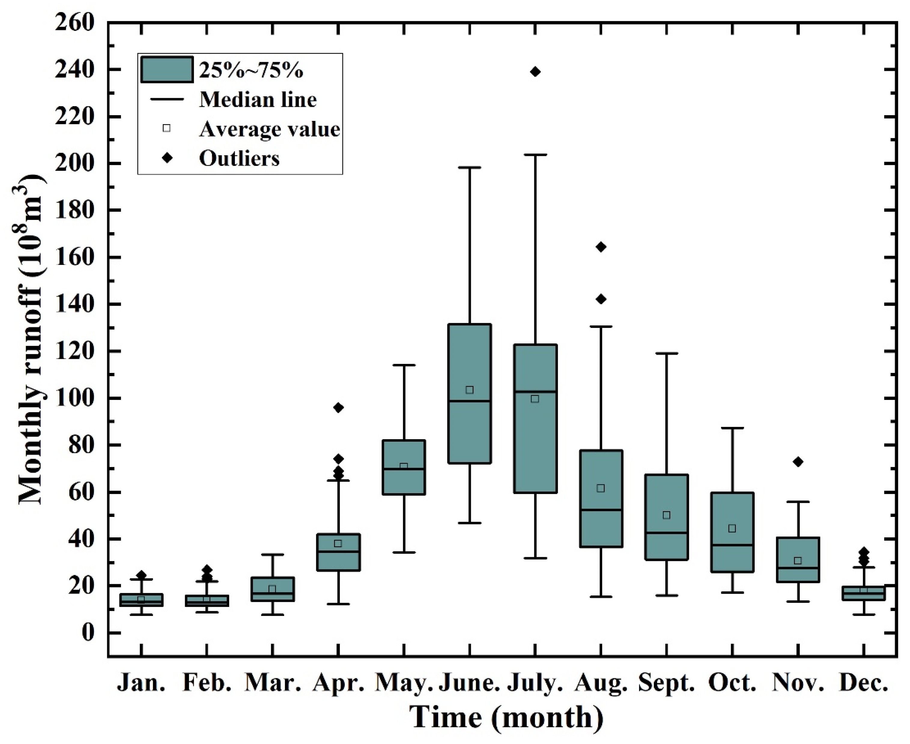
3.2.1. Monthly Scale Analysis
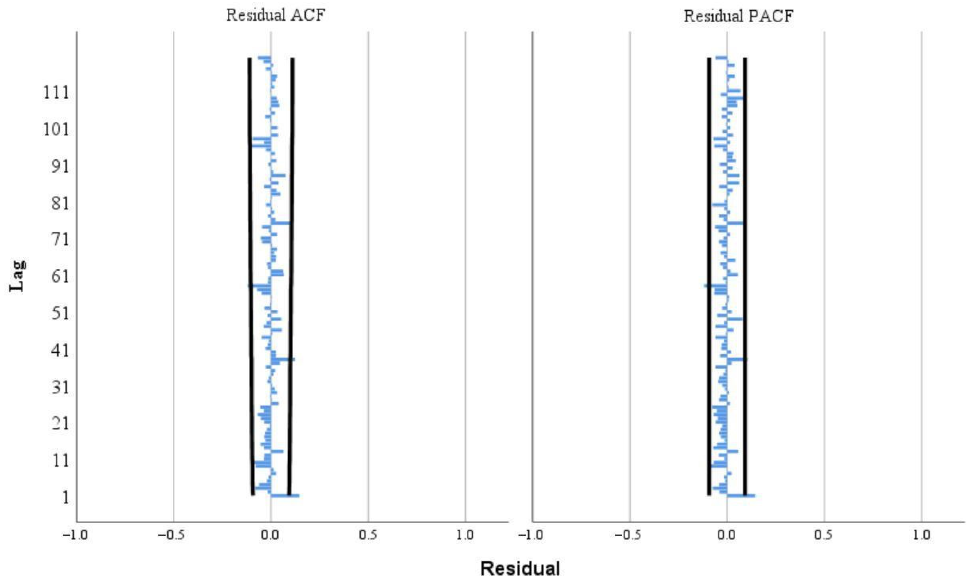
3.2.2. Time Series Analysis
4. Results and Discussion
4.1. Results
4.1.1. Predicted Results of CEEMDAN-VMD-LSTM-Informer Coupled Model
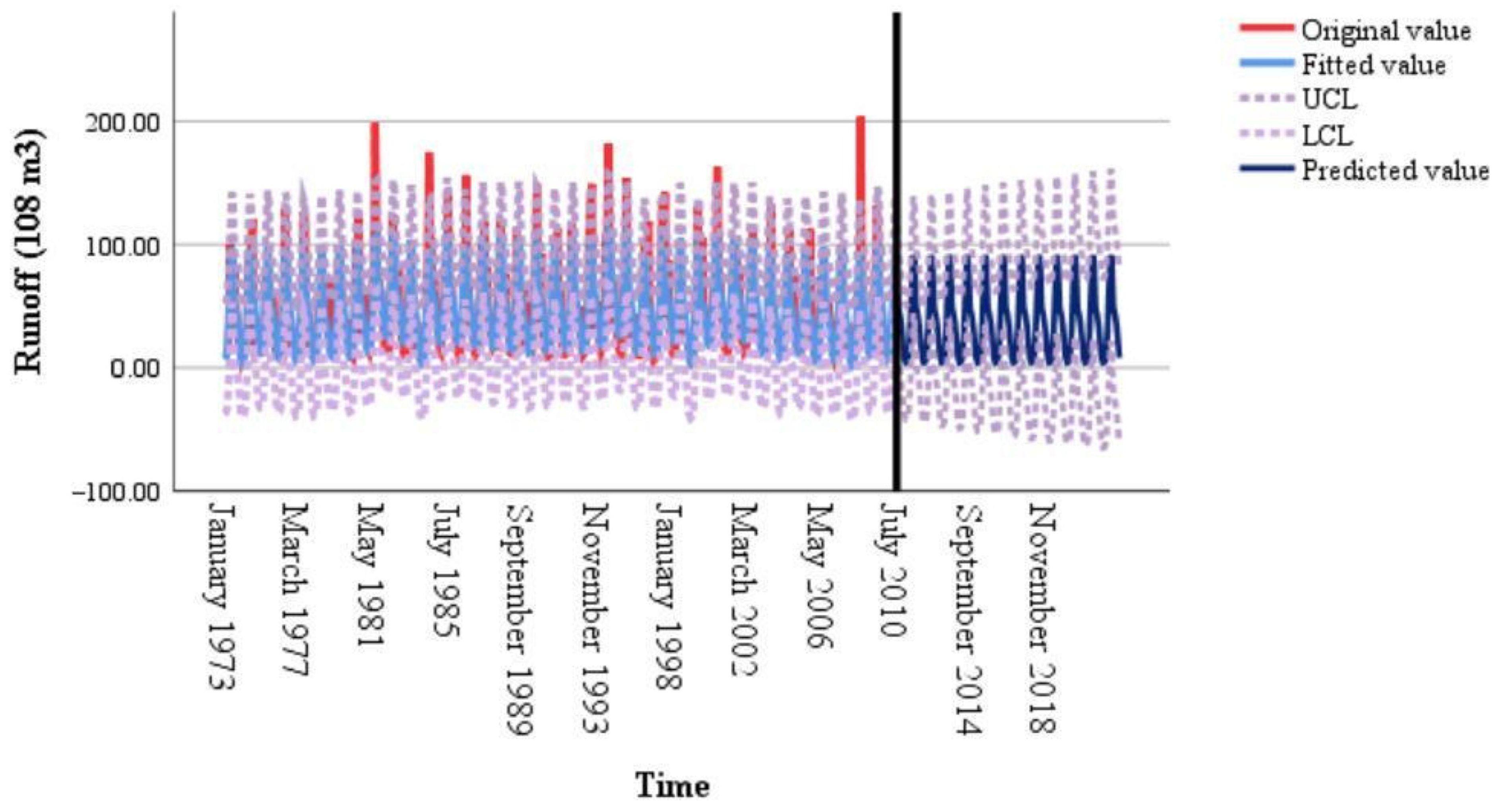
4.1.2. Predicted Results of Seasonal Exponential Smoothing Model
4.2. Discussion
5. Conclusions
- (1)
- Monthly scale runoff data at the Wulong hydrological station was a nonstationary and nonrandom sequence. The sequence showed a long-term decreasing trend and a pattern with an annual cycle. The predicted results of the seasonal exponential smoothing model showed that the prediction accuracy of the traditional statistical model is far inferior to that of machine learning models.
- (2)
- The application of the decomposition method provides a partial remedy for modal aliasing, resulting in more comprehensive and robust time series decomposition. This approach achieves a smoother monthly runoff series and reduces the interference of stochastic components with deterministic ones, ultimately enhancing the model’s predictive capabilities.
- (3)
- The combined model, which incorporates secondary decomposition, yields superior runoff prediction results. Specifically, the utilization of VMD for secondary decomposition of the highest-frequency component addresses the limitations of single-decomposition methods, resulting in a notable improvement in the accuracy of runoff predictions.
- (4)
- The CEEMDAN-VMD-LSTM-Informer model surpasses EEMD-VMD-LSTM-Informer, CEEMDAN-LSTM-Informer, CEEMDAN-LSTM, and EMD-LSTM in terms of prediction accuracy. The application of the CEEMDAN-VMD-LSTM-Informer model to monthly runoff time series prediction proves to be reliable and offers a novel approach to enhance research in monthly runoff prediction.
- (5)
- It is worth noting that this model solely considers runoff as a predictive factor. In future research endeavors, it would be advantageous to incorporate additional variables such as precipitation, evaporation, and temperature to further refine prediction accuracy.
Author Contributions
Funding
Institutional Review Board Statement
Informed Consent Statement
Data Availability Statement
Acknowledgments
Conflicts of Interest
References
- Fang, S.; Xu, L.; Pei, H.; Liu, Y.; Liu, Z.; Zhu, Y.; Yan, J.; Zhang, H. An Integrated Approach to Snowmelt Flood Forecasting in Water Resource Management. IEEE Trans. Ind. Inform. 2013, 10, 548–558. [Google Scholar] [CrossRef]
- Zhou, J.; Chen, X.; Xu, C.; Wu, P. Assessing Socioeconomic Drought Based on a Standardized Supply and Demand Water Index. Water Resour. Manag. 2022, 36, 1937–1953. [Google Scholar] [CrossRef]
- Meng, B.; Liu, J.-L.; Bao, K.; Sun, B. Water fluxes of Nenjiang River Basin with ecological network analysis: Conflict and coordination between agricultural development and wetland restoration. J. Clean. Prod. 2019, 213, 933–943. [Google Scholar] [CrossRef]
- Kurian, M. The water-energy-food nexus: Trade-offs, thresholds and transdisciplinary approaches to sustainable development. Environ. Sci. Policy 2017, 68, 97–106. [Google Scholar] [CrossRef]
- Wang, Z.; Shao, D.; Westerhoff, P. Wastewater discharge impact on drinking water sources along the Yangtze River (China). Sci. Total. Environ. 2017, 599–600, 1399–1407. [Google Scholar] [CrossRef] [PubMed]
- Dey, P.; Mishra, A. Separating the impacts of climate change and human activities on streamflow: A review of methodologies and critical assumptions. J. Hydrol. 2017, 548, 278–290. [Google Scholar] [CrossRef]
- Kotta, J.; Herkül, K.; Jaagus, J.; Kaasik, A.; Raudsepp, U.; Alari, V.; Arula, T.; Haberman, J.; Järvet, A.; Kangur, K.; et al. Linking atmospheric, terrestrial and aquatic environments: Regime shifts in the Estonian climate over the past 50 years. PLoS ONE 2018, 13, e0209568. [Google Scholar] [CrossRef] [PubMed]
- Yang, Y.; Guo, T.; Jiao, W. Destruction processes of mining on water environment in the mining area combining isotopic and hydrochemical tracer. Environ. Pollut. 2018, 237, 356–365. [Google Scholar] [CrossRef]
- Eisenmenger, N.; Pichler, M.; Krenmayr, N.; Noll, D.; Plank, B.; Schalmann, E.; Wandl, M.-T.; Gingrich, S. The Sustainable Development Goals prioritize economic growth over sustainable resource use: A critical reflection on the SDGs from a socio-ecological perspective. Sustain. Sci. 2020, 15, 1101–1110. [Google Scholar] [CrossRef]
- Hong, M.; Wang, D.; Wang, Y.; Zeng, X.; Ge, S.; Yan, H.; Singh, V.P. Mid- and long-term runoff predictions by an improved phase-space reconstruction model. Environ. Res. 2016, 148, 560–573. [Google Scholar] [CrossRef]
- Jiang, Z.; Li, R.; Li, A.; Ji, C. Runoff forecast uncertainty considered load adjustment model of cascade hydropower stations and its application. Energy 2018, 158, 693–708. [Google Scholar] [CrossRef]
- Li, W.; Kiaghadi, A.; Dawson, C. High temporal resolution rainfall–runoff modeling using long-short-term-memory (LSTM) networks. Neural Comput. Appl. 2021, 33, 1261–1278. [Google Scholar] [CrossRef]
- Wu, J.; Wang, Z.; Hu, Y.; Tao, S.; Dong, J. Runoff Forecasting using Convolutional Neural Networks and optimized Bi-directional Long Short-term Memory. Water Resour. Manag. 2023, 37, 937–953. [Google Scholar] [CrossRef]
- Bao, H.J.; Wang, L.L.; Li, Z.J.; Zhao, L.N.; Zhang, G.P. Hydrological daily rainfall-runoff simulation with BTOPMC model and comparison with Xin’anjiang model. Water Sci. Eng. 2010, 3, 121–131. [Google Scholar]
- Douglas-Mankin, K.R.; Srinivasan, R.; Arnold, J.G. Soil and Water Assessment Tool (SWAT) Model: Current Developments and Applications. Trans. ASABE 2010, 53, 1423–1431. [Google Scholar] [CrossRef]
- Mishra, S.K.; Singh, V.P. Long-term hydrological simulation based on the Soil Conservation Service curve number. Hydrol. Process. 2004, 18, 1291–1313. [Google Scholar] [CrossRef]
- Li, H.; Beldring, S.; Xu, C.-Y. Implementation and testing of routing algorithms in the distributed Hydrologiska Byråns Vattenbalansavdelning model for mountainous catchments. Hydrol. Res. 2013, 45, 322–333. [Google Scholar] [CrossRef]
- Cerdan, O.; Souchère, V.; Lecomte, V.; Couturier, A.; Le Bissonnais, Y. Incorporating soil surface crusting processes in an expert-based runoff model: Sealing and Transfer by Runoff and Erosion related to Agricultural Management. Catena 2002, 46, 189–205. [Google Scholar] [CrossRef]
- Li, K.; Huang, G.; Wang, S.; Razavi, S. Development of a physics-informed data-driven model for gaining insights into hydrological processes in irrigated watersheds. J. Hydrol. 2022, 613, 128323. [Google Scholar] [CrossRef]
- Li, F.; Ma, G.; Chen, S.; Huang, W. An ensemble modeling approach to forecast daily reservoir inflow using bidirectional long-and short-term memory (Bi-LSTM), variational mode decomposition (VMD), and energy entropy method. Water Resour. Manag. 2021, 35, 2941–2963. [Google Scholar] [CrossRef]
- Liu, K.; Chen, Y.; Zhang, X. An Evaluation of ARFIMA (Autoregressive Fractional Integral Moving Average) Programs. Axioms 2017, 6, 16. [Google Scholar] [CrossRef]
- Chen, L.; Wu, T.; Wang, Z.; Lin, X.; Cai, Y. A novel hybrid BPNN model based on adaptive evolutionary Artificial Bee Colony Algorithm for water quality index prediction. Ecol. Indic. 2023, 146, 109882. [Google Scholar] [CrossRef]
- Gong, M.; Zhao, Y.; Sun, J.; Han, C.; Sun, G.; Yan, B. Load forecasting of district heating system based on Informer. Energy 2022, 253, 124179. [Google Scholar] [CrossRef]
- Meng, E.; Huang, S.; Huang, Q.; Fang, W.; Wu, L.; Wang, L. A robust method for non-stationary streamflow prediction based on improved EMD-SVM model. J. Hydrol. 2019, 568, 462–478. [Google Scholar] [CrossRef]
- Abda, Z.; Chettih, M. Forecasting daily flow rate-based intelligent hybrid models combining wavelet and Hilbert–Huang transforms in the mediterranean basin in northern Algeria. Acta Geophys. 2018, 66, 1131–1150. [Google Scholar] [CrossRef]
- Yu, Y.; Zhang, H.; Singh, V.P. Forward Prediction of Runoff Data in Data-Scarce Basins with an Improved Ensemble Empirical Mode Decomposition (EEMD) Model. Water 2018, 10, 388. [Google Scholar] [CrossRef]
- Bae, S.; Paris, S.; Durand, F. Two-scale tone management for photographic look. ACM Trans. Graph. (TOG) 2006, 25, 637–645. [Google Scholar] [CrossRef]
- He, C.; Chen, F.; Long, A.; Qian, Y.; Tang, H. Improving the precision of monthly runoff prediction using the combined non-stationary methods in an oasis irrigation area. Agric. Water Manag. 2023, 279, 108161. [Google Scholar] [CrossRef]
- Junsheng, C.; Dejie, Y.; Yu, Y. Research on the intrinsic mode function (IMF) criterion in EMD method. Mech. Syst. Signal Process. 2006, 20, 817–824. [Google Scholar] [CrossRef]
- Fan, X.; Zhang, Y.; Krehbiel, P.R.; Zhang, Y.; Zheng, D.; Yao, W.; Xu, L.; Liu, H.; Lyu, W. Application of Ensemble Empirical Mode Decomposition in Low-Frequency Lightning Electric Field Signal Analysis and Lightning Location. IEEE Trans. Geosci. Remote. Sens. 2020, 59, 86–100. [Google Scholar] [CrossRef]
- Wu, Z.; Huang, N.E. Ensemble empirical mode decomposition: A noise-assisted data analysis method. Adv. Adapt. Data Anal. 2009, 1, 1–41. [Google Scholar] [CrossRef]
- Torres, M.E.; Colominas, M.A.; Schlotthauer, G.; Flandrin, P. A complete ensemble empirical mode decomposition with adaptive noise. In Proceedings of the 2011 IEEE International Conference on Acoustics, Speech and Signal Processing (ICASSP), Prague, Czech Republic, 22–27 May 2011; pp. 4144–4147. [Google Scholar] [CrossRef]
- Fu, W.; Shao, K.; Tan, J.; Wang, K. Fault Diagnosis for Rolling Bearings Based on Composite Multiscale Fine-Sorted Dispersion Entropy and SVM With Hybrid Mutation SCA-HHO Algorithm Optimization. IEEE Access 2020, 8, 13086–13104. [Google Scholar] [CrossRef]
- Shewalkar, A.; Nyavanandi, D.; Ludwig, S.A. Performance Evaluation of Deep Neural Networks Applied to Speech Recognition: RNN, LSTM and GRU. J. Artif. Intell. Soft Comput. Res. 2019, 9, 235–245. [Google Scholar] [CrossRef]
- Dong, M.; Grumbach, L. A Hybrid Distribution Feeder Long-Term Load Forecasting Method Based on Sequence Prediction. IEEE Trans. Smart Grid 2019, 11, 470–482. [Google Scholar] [CrossRef]
- Li, D.; Lin, K.; Li, X.; Liao, J.; Du, R.; Chen, D.; Madden, A. Improved sales time series predictions using deep neural networks with spatiotemporal dynamic pattern acquisition mechanism. Inf. Process. Manag. 2022, 59, 102987. [Google Scholar] [CrossRef]
- Chang, Y.; Li, F.; Chen, J.; Liu, Y.; Li, Z. Efficient temporal flow Transformer accompanied with multi-head probsparse self-attention mechanism for remaining useful life prognostics. Reliab. Eng. Syst. Saf. 2022, 226, 108701. [Google Scholar] [CrossRef]
- Habtemariam, E.T.; Kekeba, K.; Martínez-Ballesteros, M.; Martínez-Álvarez, F. A Bayesian Optimization-Based LSTM Model for Wind Power Forecasting in the Adama District, Ethiopia. Energies 2023, 16, 2317. [Google Scholar] [CrossRef]
- Xiaobing, Y.; Chenliang, L.; Tongzhao, H.; Zhonghui, J. Information diffusion theory-based approach for the risk assessment of meteorological disasters in the Yangtze River Basin. Nat. Hazards 2021, 107, 2337–2362. [Google Scholar] [CrossRef]
- Tamm, O.; Saaremäe, E.; Rahkema, K.; Jaagus, J.; Tamm, T. The intensification of short-duration rainfall extremes due to climate change–Need for a frequent update of intensity–duration–frequency curves. Clim. Serv. 2023, 30, 100349. [Google Scholar] [CrossRef]


| Models | Hyperparameters | Values |
|---|---|---|
| LSTM | Time step | 24 |
| Batch size | 32 | |
| Layers | 2 | |
| Hidden size | 128 | |
| Learning rate | 0.000001 | |
| Informer | Encoder layers | 2 |
| Decoder layers | 1 | |
| Multi-head attention | 8 | |
| Batch size | 16 | |
| Epochs | 20 | |
| Dropout | 0.1 |
| Models | NSE | MAE (108 m3) | MAPE (%) | RMSE (108 m3) |
|---|---|---|---|---|
| CEEMDAN-VMD-LSTM-Informer | 0.997 | 1.327 | 2.57 | 2.266 |
| EEMD-VMD-LSTM-Informer | 0.946 | 1.756 | 2.86 | 2.752 |
| CEEMDAN-LSTM-Informer | 0.926 | 2.285 | 3.15 | 3.058 |
| CEEMDAN-LSTM | 0.915 | 2.689 | 3.48 | 3.269 |
| EMD-LSTM | 0.867 | 2.952 | 4.20 | 3.681 |
| Seasonal exponential smoothing | 0.516 | 8.629 | 15.49 | 9.658 |
Disclaimer/Publisher’s Note: The statements, opinions and data contained in all publications are solely those of the individual author(s) and contributor(s) and not of MDPI and/or the editor(s). MDPI and/or the editor(s) disclaim responsibility for any injury to people or property resulting from any ideas, methods, instructions or products referred to in the content. |
© 2023 by the authors. Licensee MDPI, Basel, Switzerland. This article is an open access article distributed under the terms and conditions of the Creative Commons Attribution (CC BY) license (https://creativecommons.org/licenses/by/4.0/).
Share and Cite
Wei, H.; Wang, Y.; Liu, J.; Cao, Y. Monthly Runoff Prediction by Combined Models Based on Secondary Decomposition at the Wulong Hydrological Station in the Yangtze River Basin. Water 2023, 15, 3717. https://doi.org/10.3390/w15213717
Wei H, Wang Y, Liu J, Cao Y. Monthly Runoff Prediction by Combined Models Based on Secondary Decomposition at the Wulong Hydrological Station in the Yangtze River Basin. Water. 2023; 15(21):3717. https://doi.org/10.3390/w15213717
Chicago/Turabian StyleWei, Huaibin, Yao Wang, Jing Liu, and Yongxiao Cao. 2023. "Monthly Runoff Prediction by Combined Models Based on Secondary Decomposition at the Wulong Hydrological Station in the Yangtze River Basin" Water 15, no. 21: 3717. https://doi.org/10.3390/w15213717
APA StyleWei, H., Wang, Y., Liu, J., & Cao, Y. (2023). Monthly Runoff Prediction by Combined Models Based on Secondary Decomposition at the Wulong Hydrological Station in the Yangtze River Basin. Water, 15(21), 3717. https://doi.org/10.3390/w15213717