Article

Multi-Algorithm Hybrid Optimization of Back Propagation (BP) Neural Networks for Reference Crop Evapotranspiration Prediction Models

1
College of Mechanical and Electrical Engineering, Shihezi University, Shihezi 832003, China
2
Xinjiang Production and Construction Corps Key Laboratory of Modern Agricultural Machinery, Shihezi 832003, China
3
Key Laboratory of Northwest Agricultural Equipment, Ministry of Agriculture and Rural Affairs, Shihezi 832003, China
4
Bingtuan Energy Development Institute, Shihezi University, Shihezi 832003, China
*
Author to whom correspondence should be addressed.
Water 2023, 15(21), 3718; https://doi.org/10.3390/w15213718
Submission received: 25 September 2023 / Revised: 19 October 2023 / Accepted: 22 October 2023 / Published: 25 October 2023

Abstract

:
The reference crop evapotranspiration (ET0) statistic is useful for estimating agricultural system water requirements and managing irrigation. In dry areas, the accurate calculation of ET0 is crucial for optimal agricultural water resource utilization. By investigating the relationship between meteorological information and ET0 in Shihezi City, four prediction models were developed: a BP neural network prediction model, a BP neural network prediction model improved by genetic algorithm (GA-BP), a BP neural network prediction model improved by particle swarm algorithm (PSO-BP), as well as an improved hybrid BP neural network prediction model (GA-PSO-BP). The Pearson correlation analysis found that the key parameters influencing ET0 were temperature (Tmax, Tave, Tmin), hours of sunshine (N), relative humidity (RH), wind speed (U), as well as average pressure (AP). Based on the analysis results, different combinations of meteorological input factors were established for modeling, and the results showed that when the input factors were temperature (Tmax, Tave, Tmin), hours of sunshine (N), as well as relative humidity (RH), the overall effect of the ET0 prediction model was better than the other input combinations, and the GA-PSO-BP prediction model was the best, which could provide some guidance for the deployment and use of water resources. This may assist in the allocation and utilization of agricultural water resources in Shihezi.

1. Introduction

The wise use of water resources has a direct impact on the world’s food security and stability, yet global climate change has exacerbated the scarcity of water resources in recent years. The issue of how to realize efficient water resource utilization in the face of restricted water resources has steadily gained attention [1,2,3]. China is a large agricultural country, with a substantial share of water utilized for agricultural irrigation, and a lack of scientific supervision in the irrigation process results in irrigation water greatly surpassing crop needs [4]. The quantity of water lost by soil evaporation and vegetation transpiration during crop growth is represented by the actual crop evapotranspiration (ETa), which is calculated by multiplying the reference crop evapotranspiration (ET0) by the crop factor (Kc) [5,6]. As a result, correct calculation of ET0 will effectively alleviate problems like excess irrigation in the irrigation process [7]. The ET0 is a notion that dates back to the 1970s and was properly defined and codified in 1985. In the 1990s, a variety of equations for estimating ET0, including Penman’s combinatorial equations, were widely utilized, and studies were performed to enhance these equations. Finally, in the Expert Consultation Report on the Procedure for Revision of the FAO Guidelines for the Prediction of Water Requirements of Crops, the Food and Agriculture Organization of the United Nations (FAO) advised using the Penman–Monteith equation to estimate ET0 [8,9].
With the rapid growth of computer technology in recent years, several researchers have developed a range of basic models for estimating ET0 using machine learning, such as those based on temperature, light intensity, wind speed, and so on [10]. Kumar et al. employed an artificial neural network (ANN) to create a model for calculating the ET0 of grassland, and the findings indicated that their ANN model for forecasting was more precise than the previous method [11]. Feng et al. developed ET0 prediction models based on generalized regression neural network (GRNN) and random forest (RF) algorithms, and in each case, the findings showed that the random forest (RF) model performed marginally better compared to the GRNN model [12]. Zhang et al. built a spatially dispersed ET0 model using remote sensing data and machine learning methods, then examined its adaptability, which revealed that the method was better at estimating ET0 [13]. Bellido et al. used a number of techniques and different combinations of input variables to develop a prediction model for reference crop evapotranspiration (ET0), and the performance of the models built was comparable [14].
Shihezi is located in Northwest China’s inland region, and it is a typical dry city that has little rainfall. Agriculture is the main industry in this region, which is frequently plagued by water shortages and other difficulties affecting agricultural output. As a result, correct calculation of ET0 is critical for achieving optimal deployment and exploitation of agricultural irrigation water resources. In this paper, an ET0 prediction model based on a genetic algorithm (GA), particle swarm optimization (PSO), and BP neural network is developed by investigating the impacts of various climatic parameters on ET0 with various input combinations. The following are the specific research objectives: (1) Determine the consequences of various combinations of input elements on each day ET0 estimation in order to identify appropriate input components for modeling. (2) Create an ET0 prediction model built around a BP neural network and optimize it using a genetic algorithm (GA), a particle swarm algorithm (PSO), as well as a hybrid approach (GA-PSO). (3) The four ET0 prediction models were simulated and analyzed using MATLAB to determine the best model for agricultural productivity and water resource management in the Shihezi city.

2. Materials and Methods

2.1. Study Area and Sources of Data

Shihezi City is situated at 44°15′43″–44°19′13″ N and 85°59′12″–86°08′13″ E. It has a normal temperate continental climate. Long, cold winters and short, hot summers define the region, with yearly precipitation ranging from 125.0 to 207.7 mm and agricultural productivity reliant on irrigation. In recent years, as the region’s population has grown, the scope of agricultural output has expanded, and the amount of water needed in agriculture has increased. However, water consumption in the Shihezi region must be dispatched from other locations, and there is an imbalance between supply and demand; actualizing optimal water resource utilization in the face of scarce water supplies is critical for agricultural production in the region.
The research presented in this article is based on Shihezi City’s meteorological data for the entire year of 2022 (Table 1), which is obtained from the National Meteorological Science Data Center and includes maximum, average, and minimum temperatures (Tmax, Tave, and Tmin, °C), wind speed (U, m/s), hours of sunshine (N, h), relative humidity (RH, %), average air pressure (AP, hap), and precipitation (P, mm).
Shihezi City is a major producer of cotton, a crop that requires a lot of water. The total precipitation in Shihezi City during 2022 was only 85.3 mm, and relying on precipitation alone would not be sufficient to meet the water needs of cotton at all growth phases, thus necessitating the use of artificial irrigation. However, no current measured data for ET0 in cotton fields exist, and therefore the Penman–Monteith formula is typically employed to calculate ET0 [15,16].
ET 0 = 0.408 Δ ( R n G ) + γ 900 T + 273 U 2 ( e s e a ) Δ + γ ( 1 + 0.34 U 2 )
where: Δ denotes the slope of the saturated water vapor pressure and temperature curve (kPa/°C); Rn denotes net solar radiation (MJ·m−2·d−1); G denotes soil heat flux (MJ·m−2·d−1); T denotes the average daily air temperature (°C); γ denotes the wet and dry table constants; U2 denotes wind speed at a distance of 2 m (m/s); es denotes saturated water vapor pressure; and ea represents real water vapor pressure (kPa).

2.2. BP Neural Network

As shown in Figure 1, the BP neural network is a multilayered bidirectional network with unidirectional propagation that consists of three layers: input, hidden, and output. If the difference between the forward transmission of the learning mode that the sample data sent through the input layer into the implied layer, in the implied layer function of transfer, under the action of the output of the implied layer output signal, and the output signal, the output of the prediction results, and the real value of comparison is large, then enter the error back propagation. In contrast, error back propagation assigns the error signal layer by layer, adjusting the weights as well as thresholds of every single layer unless the error value falls within the predetermined error range or approaches the end of the pre-set number of training times and training period [17,18].
The BP neural network training process is as follows:
Step 1: Identify the number of nodes a, b, c in the BP neural network’s input, hidden, and output layers, initialize the connection weights Wij and Wjl within the neurons in each layer, given the learning rate and neuron excitation function, and initialize the hidden and output layer thresholds m, n.
Step 2: From the input quantity X and the hidden layer link weights Wij and threshold m, compute the hidden layer output. The following is the formula:
H j = F i = 1 n W i j X i m i
where F(x) is an S-type excitation function
F ( x ) = 1 1 + exp ( α x )
Step 3: Determine the output layer Ol by implicitly producing Hj and connecting the weights Wjl and the threshold n. The following is the formula:
O l = j = 1 b H j W j l n l
Step 4: Using the following formula, calculate the output error El between the expected output Ol and the intended output Tl:
E l = 1 2 l = 1 c ( T l O l )
Step 5: Use the output error El to correct the output layer and implied layer weights as follows:
W i j = W i j + η H j ( 1 H j ) X i l c W i j E l
W j l = W j l + η H j E l
where η denotes the learning coefficient.
Step 6: Adjust the threshold based on the output error El, which is determined as follows:
m j = m j + η H j ( 1 H j ) l = 1 c W j l E l
n l = n l + E l
Step 7: Check to see if the network has met the end conditions; if not, continue training.

2.3. BP Neural Networks’ Genetic Algorithm Optimization

The genetic algorithm (GA) has become a type of intelligent algorithm for optimization that uses the survival law of nature’s superiority and inferiority evolutionary process to carry out global optimization search computation. The principle is to make the population evolve through repeated selection, crossover, and mutation, and finally obtain the population’s optimal individual [19]. Because BP neural networks easily fall into local optima and have other shortcomings, optimization is performed using genetic algorithms. The fundamental concept is to encode the weights and thresholds of the implicit layer nodes as a set of chromosomes and use the selection, crossover, and mutation operations of genetic algorithms to generate a set of optimal initial weights and thresholds, and then train the generated initial values, iterating repeatedly [20,21,22].
The following is the specific procedure of genetic algorithm optimization:
Step 1: Generate N chromosomes at random, with each chromosome representing the weights and thresholds between the BP neural network’s input, hidden, and output layers.
Step 2: The function that best describes the fitness fit was chosen to be the MSE Equation (17), and the fit of the fitness function was utilized to calculate the fitness value for each chromosome.
Step 3: Using the roulette approach, choose the chromosome with the highest applicability, and the selection probability is determined as follows:
P c = f i t c i = 1 N f i t i
where N denotes the number of chromosomes; fitc denotes the fitness value of individual c; and Pc denotes the probability of individual c being selected.
Step 4: The crossover operation is performed on the chromosomes using the genuine crossover approach to produce new chromosomes utilizing the crossover probability process described below:
x i = α x i + ( 1 α ) x j x j = α x i + ( 1 α ) x i
where xi and xj denote the two paternal chromosomes; x′i and x′j denote the two child chromosomes; and α takes the value range of [0, 1].
Step 5: Mutational operations on the staining are carried out utilizing uniform mutation to generate new chromosomes distinct from the parent, and the mutational operations are as follows:
x i = x i + ( x i x max ) f ( g ) ( r > 0.5 ) x i + ( x min x i ) f ( g ) ( r 0.5 )
f ( g ) = γ ( 1 g G max ) 2
where xmax and xmin are the highest and lowest limits of xi; g is the right now number of iterations; Gmax is the highest possible number of evolutions; and γ and r have values in the range [0, 1].
Step 6: Repeat steps 3–5 until the individual with the greatest fitness level is found.

2.4. Particle Swarm Optimization for BP Neural Networks

The particle swarm algorithm (PSO) is an overall optimization technique derived from the behavior of bird flocks and fish schools. It achieves global optimization by mimicking mutual collaboration and competition among members of bird flocks and fish schools [23,24]. Each individual is treated as a particle in the PSO algorithm, and each particle has a position vector and a velocity vector, where the location vector indicates the particle’s current solution, and the velocity vector represents the particle’s moving direction. It can swiftly converge to the global optimal solution in the search space by iteratively updating the particle’s position and velocity. Because BP neural networks have flaws such as poor convergence speed, optimizing BP neural networks using PSO may increase convergence speed and lessen the likelihood of sliding towards local extremes [25,26].
The particle swarm algorithm optimization process is described below:
Step 1: Set the velocity vi, position xi, population size N, individual highest value pbest, as well as global extreme value zbest for the particle swarm.
Step 2: MSE is chosen as the fitness function to calculate the particle swarm’s initial fitness value.
Step 3: If the individual fitness value calculated in the second step is a better value, then the individual’s current position will be used as the individual’s historical optimal placement, that is, the individual extreme value pbest; otherwise, continue to maintain the current individual extreme value pbest until a better individual appears in the update.
Step 4: Change the global extreme value zbest; compare the fitness scores of pbest and zbest; if pbest’s fitness value is better, the individual optimal position will be used as the population’s historical optimal position, that is, the global extreme value; otherwise, the present global extreme value will remain in place until an improved severe value appears.
Step 5: Change the particle’s velocity v and location x using the particle swarm algorithm velocity and position update equations, which are as follows:
v i j ( t + 1 ) = ω v i j ( t ) + c 1 r 1 ( p b e s t i j ( t ) x i j ( t ) ) + c 2 r 2 ( z b e s t i j ( t ) x i j ( t ) )
x i j ( t + 1 ) = x i j ( t ) + v i j ( t + 1 )
In addition, vij(t) represents the j-dimensional velocity component of particle i evolving to generation t; xij(t) is the j-dimensional position component of particle i evolving to generation t; pbestij(t) represents the pbesti component of the best position of the j-dimensional individual of particle i evolving to generation t; and zbestij(t) represents the j-dimensional best position of the whole particle swarm evolving to generation t zbesti component.
ω represents the weight of the inertia factor; c1 and c2 constitute learning variables with a value range of (0, 2); r1 and r2 are taking the value range of (0, 1) range. The magnitude of the inertia factor ω directly impacts the particle swarm algorithm’s optimization ability. When the value of ω is bigger, the value now displays a better global search ability, while a smaller value shows a better local convergence performance, which can be calculated as follows:
ω = ω max R ( ω max ω min ) E
where ωmax and ωmin are the highest and lowest values of the inertia gravity factor, respectively; R is the at present number of iterations; and E is the overall number of iterations.
Step 6: End condition judgment of the particle swarm algorithm, based on the set end condition of the greatest number of repetitions or go after fitness value, to determine whether the finish scenario is reached; if the finish scenario is not reached, come back to the second step; alternatively, output zbest, which is the global optimal solution.

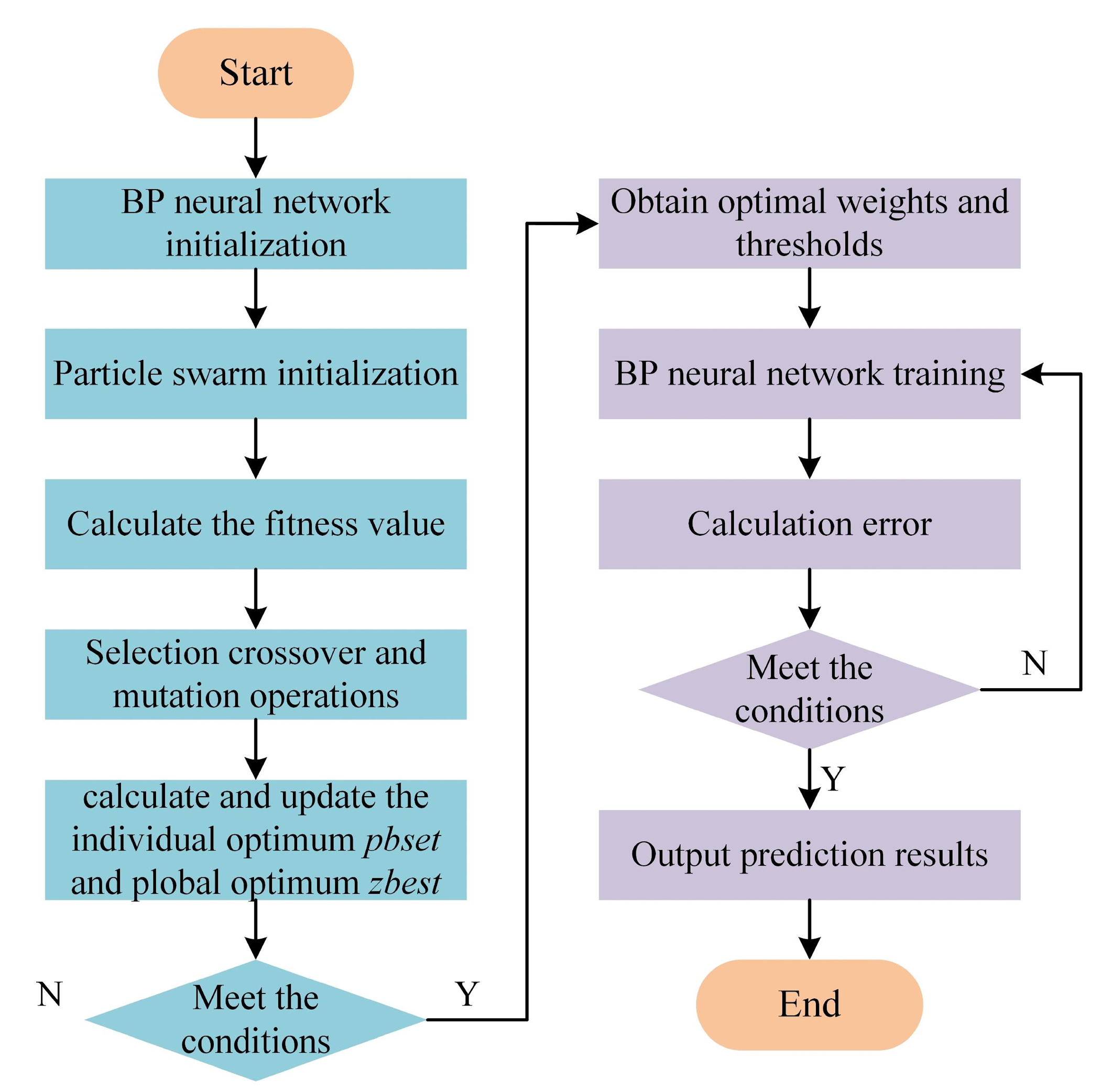
2.5. Hybrid Optimization of BP Neural Network

Both the genetic algorithm (GA) and the particle swarm algorithm (PSO) are population intelligence optimization algorithms in the subject of computer intelligence, and they have advantages and disadvantages. As a result, a hybrid GA-PSO method is developed in this research to optimize the BP neural network by including the genetic operators from the GA algorithm into the PSO algorithm. It combines the advantages of the two methods and achieves the goal of increasing the performance of the BP neural network by optimizing the BP neural network’s connection weights and assigning the optimized best weights to the BP neural network.
The following is the procedure for implementing GA-PSO optimization:
Step 1: Determine the number of nodes in the input, hidden, and output layers as well as initialize the neural network according to the model’s input and output data.
Step 2: The particle characteristics and number of particles were determined based on the network’s structure, and the speed as well as position of the particles were encoded in binary.
Step 3: MSE is implemented as the function of fitness to calculate each particle’s fitness value, and the results are utilized to determine whether the target conditions are fulfilled. If the desired circumstances are fulfilled, the results are outputted; otherwise, the particles’ individual and global optimizations are changed.
Step 4: The particle swarm crossover operation, utilizing the betting wheel approach to select better adapted particles, selected better adapted particles put into the particle swarm in the next iteration, based on the set probability of the position and speed of the particles to crossover.
Step 5: For the particle swarm mutation operation, select some of the particles from the particle swarm with low fitness values, use the velocity mutation operator and position mutation operator to mutate the velocity as well as the position of the particles based on the set probability, and reintroduce the mutated particles into the original particle swarm.
Step 6: The fitness function is used to determine the fitness value, update the individual particle polarity pbest, and update the particle swarm’s global polarity zbest.
Step 7: Determine whether the particle swarm’s fitness value meets the target value or whether the particles’ evolutionary generation is up to the greatest evolutionary generation; when the above conditions are fulfilled, then output the best possible result zbest; otherwise, proceed to the third step to finish the iteration.
Step 8: After the iteration is finished, decode the best possible result and replace the initial weights and thresholds in the specified BP neural network.
In summary, the flow of GA-PSO-BP algorithm designed in this paper is shown in Figure 2.

2.6. Criteria for Evaluation

In this study, the sample data is divided into training and test sets, with the training set accounting for 75% of total samples and the testing set accounting for 25% of total samples. The rating metrics mean absolute error (MAE), root mean square error (RMSE), and coefficient of determination (R2) are introduced for assessing the efficiency of the BP, GA-BP, PSO-BP, and GA-PSO-BP models.
MAE = 1 n i = 1 n Y i Y i
RMSE = 1 n i = 1 n ( Y i Y i ) 2
R 2 = i = 1 n ( Y i y i ) ( Y i y i ) 2 i = 1 n ( Y i y i ) 2 i = 1 n ( Y i y i ) 2
Among them, the mean absolute error (MAE) is the median of the absolute variations among the predicted and true values; the lower the MAE, the better the performance. The average square root of the difference between the anticipated and true values is the root mean square error (RMSE); the lower the RMSE, the better the performance. The coefficient of determination (R2), which has a range of [0, 1], reflects the correlation among the expected outcome and the actual result; when R2 is close to 1, the model has a stronger predictive capacity. Where Yi is the predicted value, Yi is the real value, yi is the predicted value’s average, yi represents the real value’s average, and n represents the total amount of the real value.

3. Results

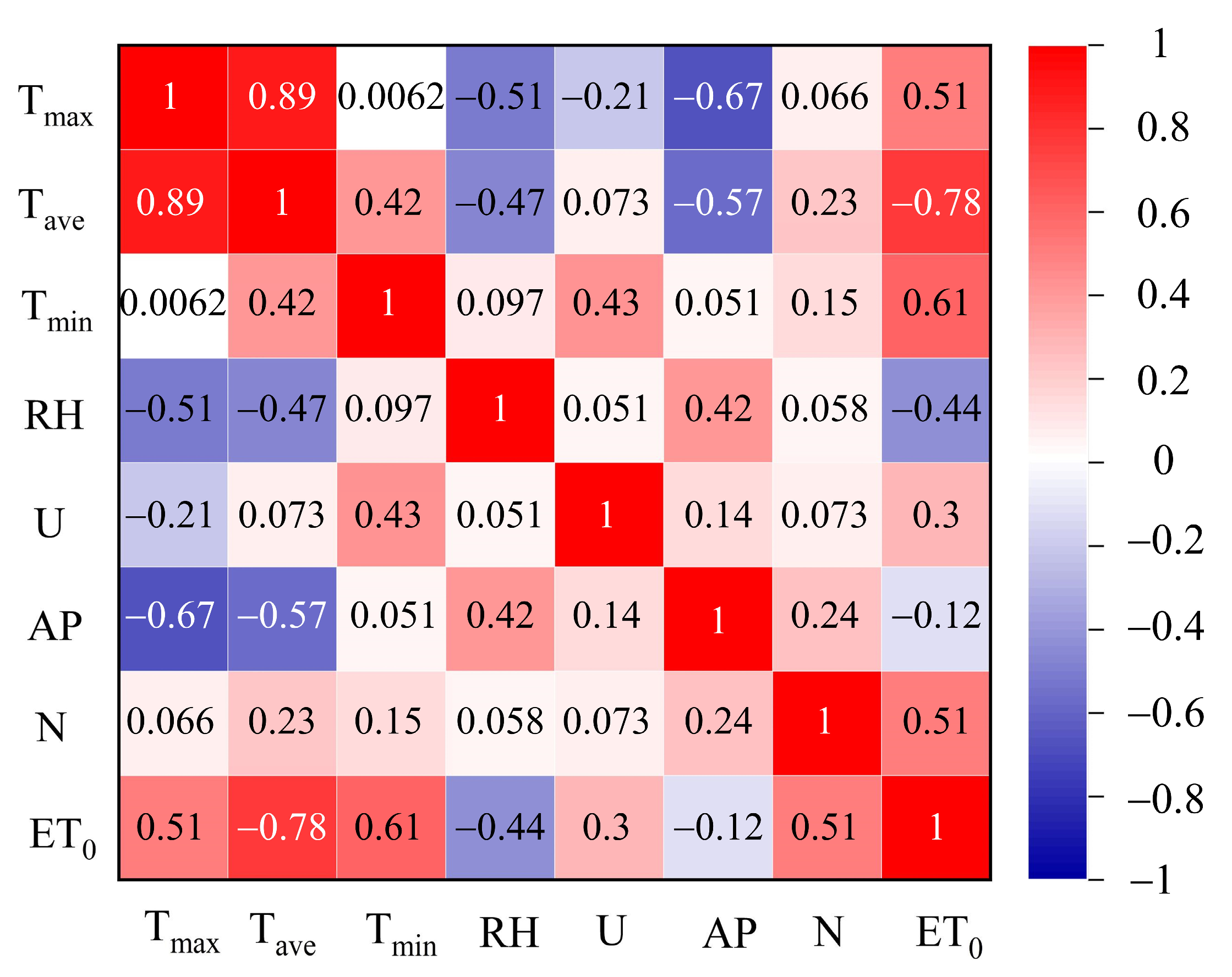
3.1. Correlation Analysis between ET0 and Meteorological Factors

The diversity of meteorological parameters and their influence on reference crop evapotranspiration (ET0) must be considered when researching the relationship between various meteorological factors and ET0. Excessive consideration of climatic parameters raises computational costs, diminishes model computational efficiency, and may reduce prediction accuracy. To determine the association between climatic parameters and ET0, a Pearson correlation analysis was utilized. Pearson correlation analysis is a statistical method for determining the degree of linearity between two variables that are continuous, and the correlation factor ranges from −1 to 1. When the absolute value approaches one, the correlation is stronger, and the positive and negative signs reflect the direction of the correlation. The presence of a positive correlation indicates that the two variables have an advantageous linear link, an unfavorable correlation indicates that the two variables have a linear connection that is unfavorable, and a correlation value close to 0 indicates that the two variables have essentially no linear connection between them.
Figure 3 depicts the correlation coefficients between meteorological factors and ET0, with maximum temperature (Tmax), average temperature (Tave), and minimum temperature (Tmin) having correlation coefficients of 0.51, 0.78, and 0.61, respectively, while hours of sunshine (N), wind speed (U), average pressure (AP), and relative humidity (RH) having correlation coefficients of 0.51, 0.3, −0.12 and −0.44. Temperature (Tmax, Tave, Tmin), wind speed (U), and hours of sunshine (N) are all positively connected with ET0, with a substantial association, although average air pressure (AP) and relative humidity (RH) are negatively correlated. However, mean air pressure (AP) has a weak association and is not used in the model’s input component selection.

3.2. Simulation Analysis of ET0 Prediction Model

To estimate daily ET0, seven distinct combinations of meteorological input factor combinations and models were chosen in this article. Temperature (Tmax, Tave, Tmin) was chosen as the first three input elements for the prediction model since it has the strongest association with ET0. Modeling simulation analysis was performed using MATLAB 2017b to assess the performance of the BP neural network prediction model, GA-BP prediction model, PSO-BP prediction model, and GA-PSO-BP prediction model under seven combinations of inputs, and the results are given in Table 2.
Table 2 shows that when the input factors are only temperature (Tmax, Tave, Tmin), the MAR, RMSE, and R2 of the model are in the ranges of 0.209–0.411 mm/day, 0.258–0.435 mm/day, and 0.793–0.893, respectively, and when the input factors are increased to 4, the MAR, RMSE, and R2 of the model are in the ranges of 0.174–0.393 mm/day, 0.212–0.401 mm/day and 0.802–0.901. When the number of input components is raised to 5, the model’s MAR, RMSE, and R2 range from 0.145 to 0.341 mm/day, 0.163 to 0.352 mm/day, and 0.843 to 0.952.

3.3. Analysis of Results

By comparing the combinations X1, X2, X3 and X4, it can be seen that the model’s effect is improved with the increase in input factors, and the superposition of sunshine hours (N), relative humidity (RH), wind speed (U) and temperature (Tmax, Tave, Tmin) all help to improve the model performance. Further comparison of combinations X5, X6 and X7 shows that the superposition of N, RH and T (Tmax, Tave, Tmin) is more effective in improving the model performance, and the model effect of combination X7 is optimal compared to other groups. The comparison of the four prediction models is shown in Figure 4.
Figure 4 depicts the overall accuracy box plots of the four prediction models, with a lower median line indicating a higher accuracy prediction of the model when MAE and RMSE have been utilized to evaluate the model. Figure 4a,b show that the BP neural network prediction model has the highest median line, while the GA-BP prediction model has a lower median line than the BP neural network prediction model, but a slightly higher median line than the PSO-BP prediction model, and the GA-PSO-BP prediction model has the lowest median line. This shows that GA and PSO can significantly enhance model prediction. When using R2 to evaluate the performance of a prediction model, the greater the median line, greater the prediction ability of the model, as shown in Figure 4c, and the lowest median line is for the BP neural network prediction model, indicating that the optimization of BP neural networks by GA-PSO is the best.

4. Discussion

The correlation between meteorological factors and reference crop evapotranspiration (ET0) is critical in determining the selection of input factors for prediction models, and many studies show that temperature crop input factors are better suited for ET0 prediction modeling in the Shihezi region [27]. This is consistent with Rachid et al.’s findings that temperature is a crucial factor regulating ET0 [28]. However, in the case of limited input factors, the performance of the prediction model built solely on the neural network is poor; having said that, the performance of the model can be improved by introducing other optimization algorithms, and it has been demonstrated that the accuracy of the optimized BP neural network is significantly higher than that of the unoptimized prediction model [29,30,31]. These findings are congruent with the findings of our investigation.
Analyzing Table 2 and Figure 4 proceeds to show that the median values of MAE, RMSE and R2 for the BP neural network prediction model are 0.349 mm/day, 0.369 mm/day, and 0.835, respectively. The GA-BP reference crop evapotranspiration prediction model has median MAE, RMSE, and R2 values of 0.258 mm/day, 0.283 mm/day, and 0.876, respectively. For the PSO-BP reference, the crop evapotranspiration model’s median MAE, RMSE, and R2 values were 0.248 mm/day, 0.277 mm/day, and 0.882, respectively. For the GA-PSO-BP reference crop evapotranspiration prediction model, the median MAE, RMSE, and R2 values were 0.174 mm/day, 0.212 mm/day, and 0.921, respectively. When compared to the BP reference crop evapotranspiration prediction model, the GA-PSO-BP reference crop evapotranspiration prediction model lowered MAE and RMSE by 50.143% and 42.547%, respectively, and improved R2 by 10.299%. MAE and RMSE were lowered by 32.558% and 25.088%, respectively, when compared to the GA-BP reference crop evapotranspiration prediction model, while R2 was increased by 5.136%. When compared to the PSO-BP reference crop evapotranspiration prediction model, MAE and RMSE were lowered by 28.868% and 23.466%, respectively, and R2 was improved by 4.422%. The GA-PSO-BP prediction model outperformed the BP neural network prediction model, the GA-BP prediction model, and the PSO-BP prediction model, and model performance was optimized when temperature (Tmax, Tave, Tmin), hours of sunlight (N), and relative humidity (RH) were input factors.

5. Conclusions

Due to the weaknesses of the BP neural network, such as a slow rate of convergence as well as the simple tumble into the optimal solution, three algorithms were used in this paper to refer to the crop evapotranspiration (ET0) prediction model: the genetic algorithm (GA), particle swarm algorithm (PSO), and hybrid optimization. The influencing elements having the highest association with ET0 were found using correlation analysis, and the ET0 prediction model was constructed and simulated using various combinations of meteorological factors. It is summarized below:
  • Temperature (Tmax, Tave, Tmin), hours of sunlight (N), relative humidity (RH), wind speed (U), and average air pressure (AP) all had an effect on reference crop evapotranspiration (ET0). And when the input factors include temperature (Tmax, Tave, Tmin), daylight hours (N), and relative humidity (RH), the model performance is better than other input combinations, indicating that this input combination is optimum for building the model.
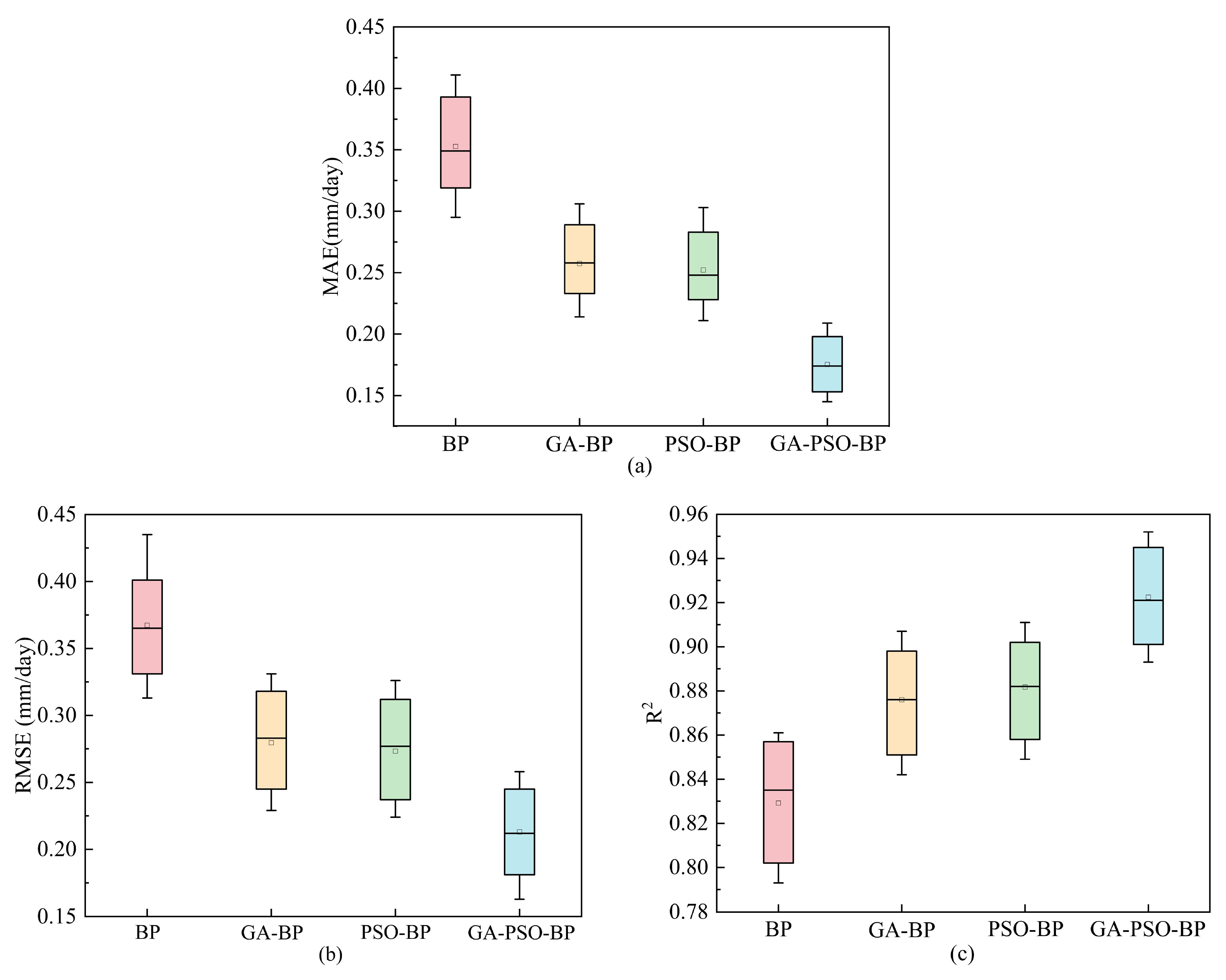
  • When the four ET0 prediction models are compared under the combination of X7 input factors, the GA-PSO-BP prediction model outperforms the other three prediction models, with optimal MAE, RMSE, and R2 values of 0.145 mm/day, 0.163 mm/day, and 0.952, respectively.
  • Analyzing seven sets of meteorological factors input combinations reveals that the hybrid algorithm (GA-PSO) provides the best performance boost to the BP neural network, and the prediction impact of the GA-PSO-BP model is optimal under each input combination. As a result, when meteorological circumstances are constrained, the use of the GA-PSO-BP model to estimate ET0 for water resource allocation has a significant reference value.
This study shows that utilizing the optimization technique of a BP neural network to develop a model to forecast reference crop evapotranspiration with only climate data as input is feasible. This is beneficial in some areas and nations when meteorological data is limited. The prediction model will be coupled with the actual irrigation process of the farmland in a future study to precisely estimate the farmland’s water demand and, finally, realize the effective use of agricultural water resources.

Author Contributions

Conceptualization, Y.Z. and L.Z.; software design, Y.Z.; software validation, Y.Z.; resources, X.H. and W.D.; data curation, J.Z. and F.Z.; writing—original draft, Y.Z.; writing—review and editing, Y.Z. and H.W. All authors have read and agreed to the published version of the manuscript.

Funding

This research was funded by National Key R&D Program of China (No. 2022ZD0115804), Xinjiang Agricultural Machinery R&D, Manufacturing, Promotion and Application Integration Project (No. YTHSD2022-03), National Natural Science Foundation of China (No. 52065055).

Data Availability Statement

Not applicable.

Conflicts of Interest

The authors declare no conflict of interest.

References

  1. Neissi, L.; Albaji, M.; Nasab, S.B. Site Selection of Different Irrigation Systems Using an Analytical Hierarchy Process Integrated with GIS in a Semi-Arid Region. Water Resour. Manag. 2019, 33, 4955–4967. [Google Scholar] [CrossRef]
  2. Marsal, J.; Girona, J.; Casadesus, J.; Lopez, G.; Stöckle, C.O. Crop coefficient (Kc) for apple: Comparison between measurements by a weighing lysimeter and prediction by CropSyst. Irrig. Sci. 2013, 31, 455–463. [Google Scholar] [CrossRef]
  3. Mokhtar, A.; Al-Ansari, N.; El-Ssawy, W.; Graf, R.; Aghelpour, P.; He, H.M.; Hafez, S.M.; Abuarab, M. Prediction of Irrigation Water Requirements for Green Beans-Based Machine Learning Algorithm Models in Arid Region. Water Resour. Manag. 2023, 37, 1557–1580. [Google Scholar] [CrossRef]
  4. Shen, J.L.; Zhao, Y.K.; Song, J.F. Analysis of the regional differences in agricultural water poverty in China: Based on a new agricultural water poverty index. Agric. Water Manag. 2022, 270, 107745. [Google Scholar] [CrossRef]
  5. Xiang, K.Y.; Li, Y.; Horton, R.; Feng, H. Similarity and difference of potential evapotranspiration and reference crop evapotranspiration—A review. Agric. Water Manag. 2020, 232, 106043. [Google Scholar] [CrossRef]
  6. Fan, J.L.; Wu, L.F.; Zhang, F.C.; Xiang, Y.Z.; Zheng, J. Climate change effects on reference crop evapotranspiration across different climatic zones of China during 1956–2015. J. Hydrol. 2016, 542, 923–937. [Google Scholar] [CrossRef]
  7. Subedi, A.; Chávez, J. Crop Evapotranspiration (ET) Estimation Models: A Review and Discussion of the Applicability and Limitations of ET Methods. J. Agric. Sci. 2015, 7, 6. [Google Scholar] [CrossRef]
  8. Pereira, L.S.; Allen, R.G.; Smith, M.; Raes, D. Crop evapotranspiration estimation with FAO56: Past and future. Agric. Water Manag. 2015, 147, 4–20. [Google Scholar] [CrossRef]
  9. Anderson, R.G.; French, A.N. Crop Evapotranspiration. Agronomy 2019, 9, 614. [Google Scholar] [CrossRef]
  10. Rodrigues, G.C.; Braga, R.P. Estimation of Reference Evapotranspiration during the Irrigation Season Using Nine Temperature-Based Methods in a Hot-Summer Mediterranean Climate. Agriculture 2021, 11, 124. [Google Scholar] [CrossRef]
  11. Kumar, M.; Raghuwanshi, N.S.; Singh, R. Artificial neural networks approach in evapotranspiration modeling: A review. Irrig. Sci. 2011, 29, 11–25. [Google Scholar] [CrossRef]
  12. Feng, Y.; Cui, N.B.; Gong, D.Z.; Zhang, Q.W.; Zhao, L. Evaluation of random forests and generalized regression neural networks for daily reference evapotranspiration modelling. Agric. Water Manag. 2017, 193, 163–173. [Google Scholar] [CrossRef]
  13. Zhang, Z.X.; Gong, Y.C.; Wang, Z.J. Accessible remote sensing data based reference evapotranspiration estimation modelling. Agric. Water Manag. 2018, 210, 59–69. [Google Scholar] [CrossRef]
  14. Bellido-Jimenez, J.A.; Estevez, J.; Garcia-Marin, A.P. New machine learning approaches to improve reference evapotranspiration estimates using intra-daily temperature-based variables in a semi-arid region of Spain. Agric. Water Manag. 2021, 245, 106588. [Google Scholar] [CrossRef]
  15. Shiri, J.; Nazemi, A.H.; Sadraddini, A.A.; Landeras, G.; Kisi, O.; Fard, A.F.; Marti, P. Comparison of heuristic and empirical approaches for estimating reference evapotranspiration from limited inputs in Iran. Comput. Electron. Agric. 2014, 108, 230–241. [Google Scholar] [CrossRef]
  16. Feng, Y.; Jia, Y.; Cui, N.B.; Zhao, L.; Li, C.; Gong, D.Z. Calibration of Hargreaves model for reference evapotranspiration estimation in Sichuan basin of southwest China. Agric. Water Manag. 2017, 181, 1–9. [Google Scholar] [CrossRef]
  17. Qi, W.; Zhang, Z.Y.; Wang, C.; Huang, M.Y. Prediction of infiltration behaviors and evaluation of irrigation efficiency in clay loam soil under Moistube (R) irrigation. Agric. Water Manag. 2021, 248, 106756. [Google Scholar] [CrossRef]
  18. Chen, R.Y.; Song, J.J.; Xu, M.B.; Wang, X.L.; Yin, Z.; Liu, T.Q.; Luo, N. Prediction of the corrosion depth of oil well cement corroded by carbon dioxide using GA-BP neural network. Constr. Build. Mater. 2023, 394, 132127. [Google Scholar] [CrossRef]
  19. Yu, A.X.; Liu, Y.K.; Li, X.; Yang, Y.L.; Zhou, Z.W.; Liu, H.R. Modeling and Optimizing of NH4+ Removal from Stormwater by Coal-Based Granular Activated Carbon Using RSM and ANN Coupled with GA. Water 2021, 13, 608. [Google Scholar] [CrossRef]
  20. Zhu, F.L.; Zhang, L.X.; Hu, X.; Zhao, J.W.; Meng, Z.H.; Zheng, Y. Research and Design of Hybrid Optimized Backpropagation (BP) Neural Network PID Algorithm for Integrated Water and Fertilizer Precision Fertilization Control System for Field Crops. Agronomy 2023, 13, 1423. [Google Scholar] [CrossRef]
  21. Singh, N.K.; Singh, Y.; Kumar, S.; Upadhyay, R. Integration of GA and neuro-fuzzy approaches for the predictive analysis of gas-assisted EDM responses. Appl. Sci. 2019, 2, 137. [Google Scholar] [CrossRef]
  22. Wang, T.; Fang, G.H.; Xie, X.M.; Liu, Y.; Ma, Z.Z. A Multi-Dimensional Equilibrium Allocation Model of Water Resources Based on a Groundwater Multiple Loop Iteration Technique. Water 2017, 9, 718. [Google Scholar] [CrossRef]
  23. Yi, W.Z. Forecast of agricultural water resources demand based on particle swarm algorithm. Acta Agric. Scand. Sect. B-Soil Plant Sci. 2022, 72, 30–42. [Google Scholar] [CrossRef]
  24. Lu, G.Y.; Xu, D.; Meng, Y. Dynamic Evolution Analysis of Desertification Images Based on BP Neural Network. Comput. Intell. Neurosci. 2022, 2022, 5645535. [Google Scholar] [CrossRef] [PubMed]
  25. Yan, J.Z.; Xu, Z.B.; Yu, Y.C.; Xu, H.X.; Gao, K.L. Application of a Hybrid Optimized BP Network Model to Estimate Water Quality Parameters of Beihai Lake in Beijing. Appl. Sci. 2019, 9, 1863. [Google Scholar] [CrossRef]
  26. Jahandideh-Tehrani, M.; Bozorg-Haddad, O.; Loaiciga, H.A. Application of particle swarm optimization to water management: An introduction and overview. Environ. Monit. Assess. 2020, 192, 281. [Google Scholar] [CrossRef]
  27. Jiao, P.; Hu, S.-J. Optimal Alternative for Quantifying Reference Evapotranspiration in Northern Xinjiang. Water 2022, 14, 1. [Google Scholar] [CrossRef]
  28. Hadria, R.; Benabdelouhab, T.; Lionboui, H.; Salhi, A. Comparative assessment of different reference evapotranspiration models towards a fit calibration for arid and semi-arid areas. J. Arid Environ. 2021, 184, 104318. [Google Scholar] [CrossRef]
  29. Qin, A.; Fan, Z.; Zhang, L. Hybrid Genetic Algorithm−Based BP Neural Network Models Optimize Estimation Performance of Reference Crop Evapotranspiration in China. Appl. Sci. 2022, 12, 10689. [Google Scholar] [CrossRef]
  30. Kim, S.; Kim, H. Neural networks and genetic algorithm approach for nonlinear evaporation and evapotranspiration modeling. J. Hydrol. 2008, 351, 299–317. [Google Scholar] [CrossRef]
  31. Zhang, Z.-C.; Zeng, X.-M.; Li, G.; Lu, B.; Xiao, M.-Z.; Wang, B.-Z. Summer Precipitation Forecast Using an Optimized Artificial Neural Network with a Genetic Algorithm for Yangtze-Huaihe River Basin, China. Atmosphere 2022, 13, 929. [Google Scholar] [CrossRef]
Figure 1. A BP neural network structure is illustrated.
Water 15 03718 g001
Figure 2. Flowchart of the GA-PSO-BP algorithm is illustrated.
Water 15 03718 g002
Figure 3. Correlation analysis of meteorological factors with ET0 are presented; Tmax, Tave, and Tmin denote maximum, average, and minimum temperatures (°C); RH denotes relative humidity (%); U denotes wind speed (m/s); AP denotes average air pressure (hap); and N denotes hours of sunshine (h).
Water 15 03718 g003
Figure 4. Box plots of the overall accuracy of the prediction model are presented: (a) mean absolute error (MAE) box plot, (b) root mean square error (RMSE) box plot, and (c) coefficient of determination (R2) box plot.
Water 15 03718 g004
Table 1. Shown below is the monthly meteorological data for Shihezi City during 2022.
MonthTmax (°C)Tave (°C)Tmin (°C)U (m/s)N (h)RH (%)AP (hap)
Jan−2.0−12.8−23.50.9290.082974
Feb4.3−12.6−25.20.829478977
Mar164.2−13.11.3370.374968
Apr30.215.5−1.51.5430.635966
May34.623.510.82.0457.040959
Jun39.926.312.31.6462.043956
Jul37.125.913.11.6467.446955
Aug35.623.47.11.4432.551959
Sep39.519.74.01.2375.247962
Oct22.88.7−2.71.0341.262971
Nov13.0−0.7−27.71.0290.580973
Dec−5.0−16.0−26.00.7278.581983
Table 2. Performance of each prediction model for 7 input combinations is reported.
InputMAE (mm/day)RMSE (mm/day)R2
X1TBP0.4110.4350.793
GA-BP0.3060.3310.842
PSO-BP0.3030.3260.849
GA-PSO-BP0.2090.2580.893
X2T, UBP0.3930.4010.802
GA-BP0.2890.3180.851
PSO-BP0.2830.3120.858
GA-PSO-BP0.1980.2450.901
X3T, RHBP0.3610.3740.813
GA-BP0.2610.2950.869
PSO-BP0.2550.2860.877
GA-PSO-BP0.1830.2310.912
X4T, NBP0.3490.3650.835
GA-BP0.2580.2830.876
PSO-BP0.2480.2770.882
GA-PSO-BP0.1740.2120.921
X5T, RH, UBP0.3410.3520.843
GA-BP0.2410.2560.889
PSO-BP0.2370.2510.893
GA-PSO-BP0.1650.2010.933
X6T, N, UBP0.3190.3310.857
GA-BP0.2330.2450.898
PSO-BP0.2280.2370.902
GA-PSO-BP0.1530.1810.945
X7T, N, RHBP0.2950.3130.871
GA-BP0.2140.2290.907
PSO-BP0.2110.2240.911
GA-PSO-BP0.1450.1630.952
Note: T (°C) denote maximum temperature (Tmax), average temperature (Tave), and minimum temperature (Tmin); RH denotes relative humidity (%); U denotes wind speed (m/s); AP denotes average air pressure (hap); and N denotes hours of sunshine (h).
Disclaimer/Publisher’s Note: The statements, opinions and data contained in all publications are solely those of the individual author(s) and contributor(s) and not of MDPI and/or the editor(s). MDPI and/or the editor(s) disclaim responsibility for any injury to people or property resulting from any ideas, methods, instructions or products referred to in the content.

