


Groundwater Storage Variations in the Main Karoo Aquifer Estimated Using GRACE and GPS


Abstract
:1. Introduction
2. Materials
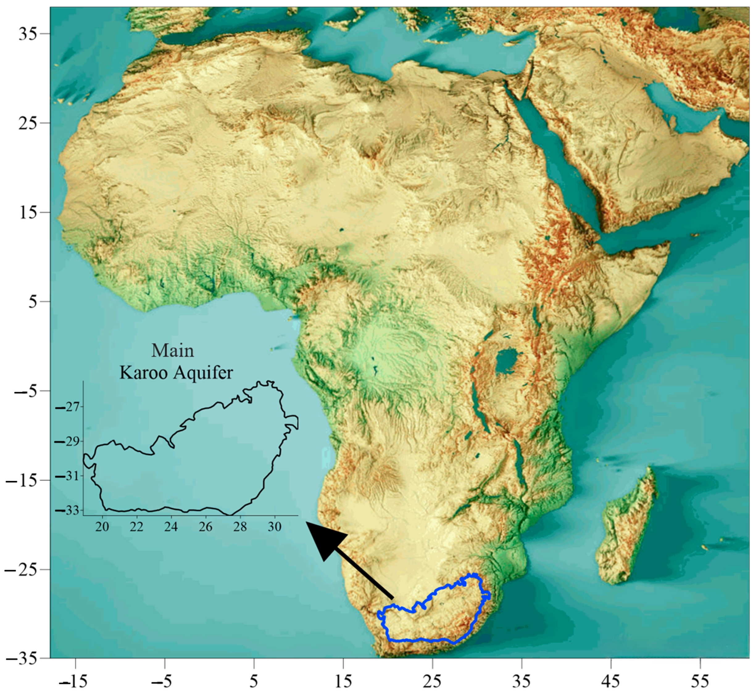
2.1. Study Area
2.2. GPS Data
2.3. GRACE Data
2.4. Global Land Data Assimilation System (GLDAS)
2.5. WaterGAP Global Hydrology Model (WGHM)
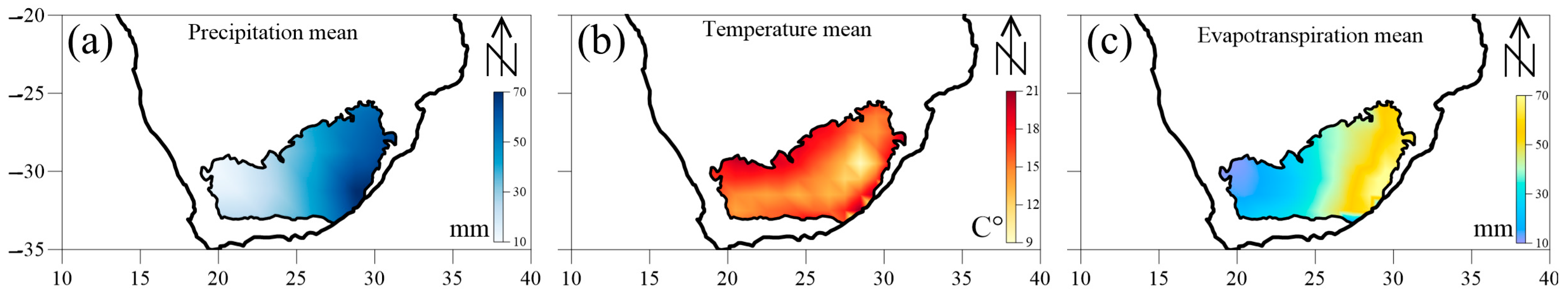
2.6. Precipitation and Air Temperature
3. Methods
3.1. GWS Estimation
- (1)
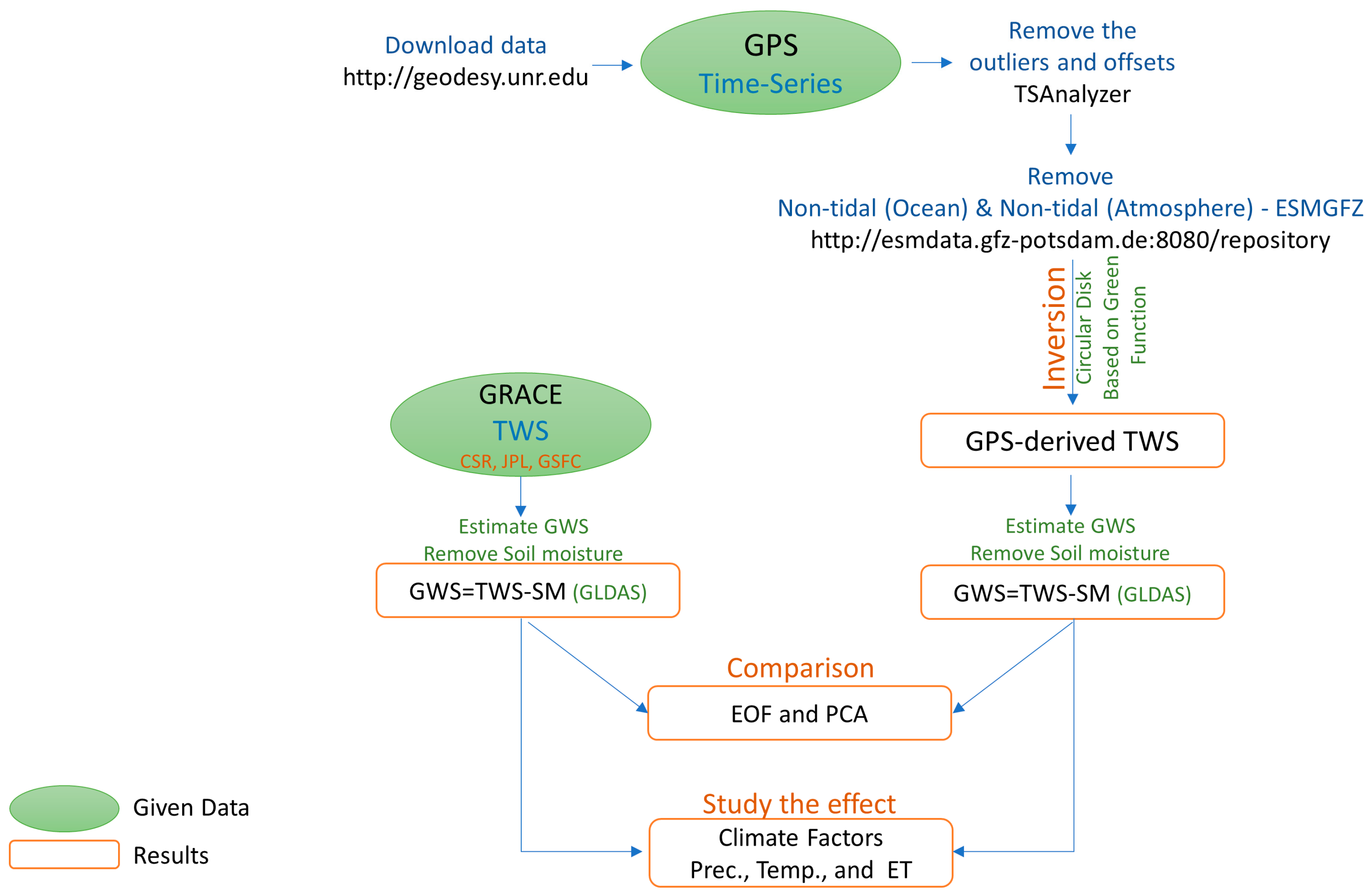
- We used the TSAnalyzer software to eliminate outliers and offsets from the raw GPS time series (https://github.com/wudingcheng/TSAnalyzer/, accessed on 20 January 2023).
- (2)
- To ascertain vertical crustal deformation tied to seasonal TWS fluctuations, non-tidal atmospheric loading (NTAL) and non-tidal ocean loading (NTOL) influences were averaged into daily results and removed using the product repository by Deutsches GeoForschungsZentrum (GFZ) (http://esmdata.gfz-potsdam.de:8080/repository, accessed on 20 January 2023) [49].
- (3)
- The preceding two steps prepared the GPS data for inversion through a circular disk and the Green function, converting it into TWS according to the mass loading inversion method illustrated in the next section.
- (4)
- After obtaining the GPS-derived TWS, the soil moisture anomaly was also calculated from GLDAS-2.1 Noah model as was done with the GRACE data (Equation (3)). Then the GPS-derived GWS can be estimated by removing soil moisture anomaly from the GPS-derived TWS (Equation (2)).
3.2. Mass Loading Inversion Method
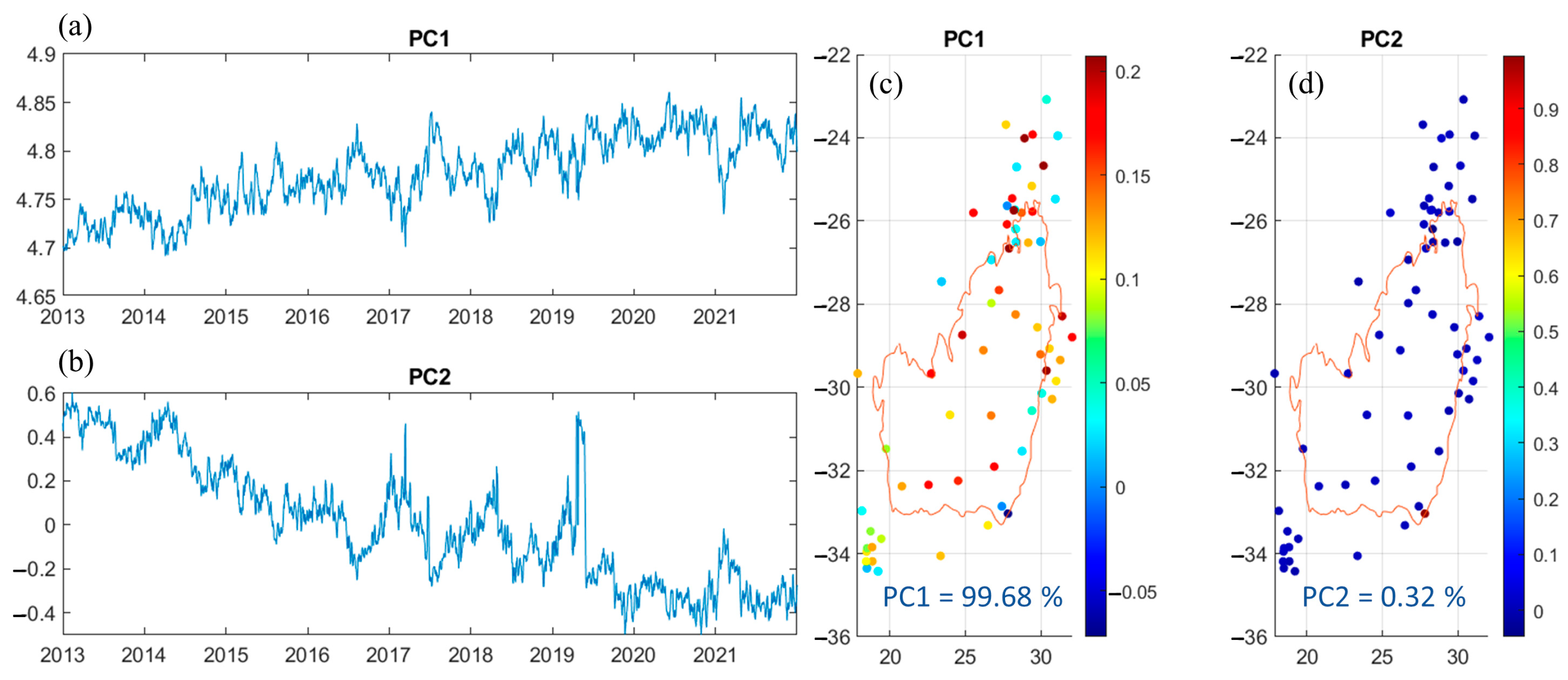
3.3. Principle Component Analysis (PCA)
4. Results
4.1. GPS Inversion and Model Resolution Test
4.2. Groundwater Storage (GWS)
5. Discussion
5.1. Comparison between GPS and GRACE-Derived GWS
5.1.1. EOF Modes
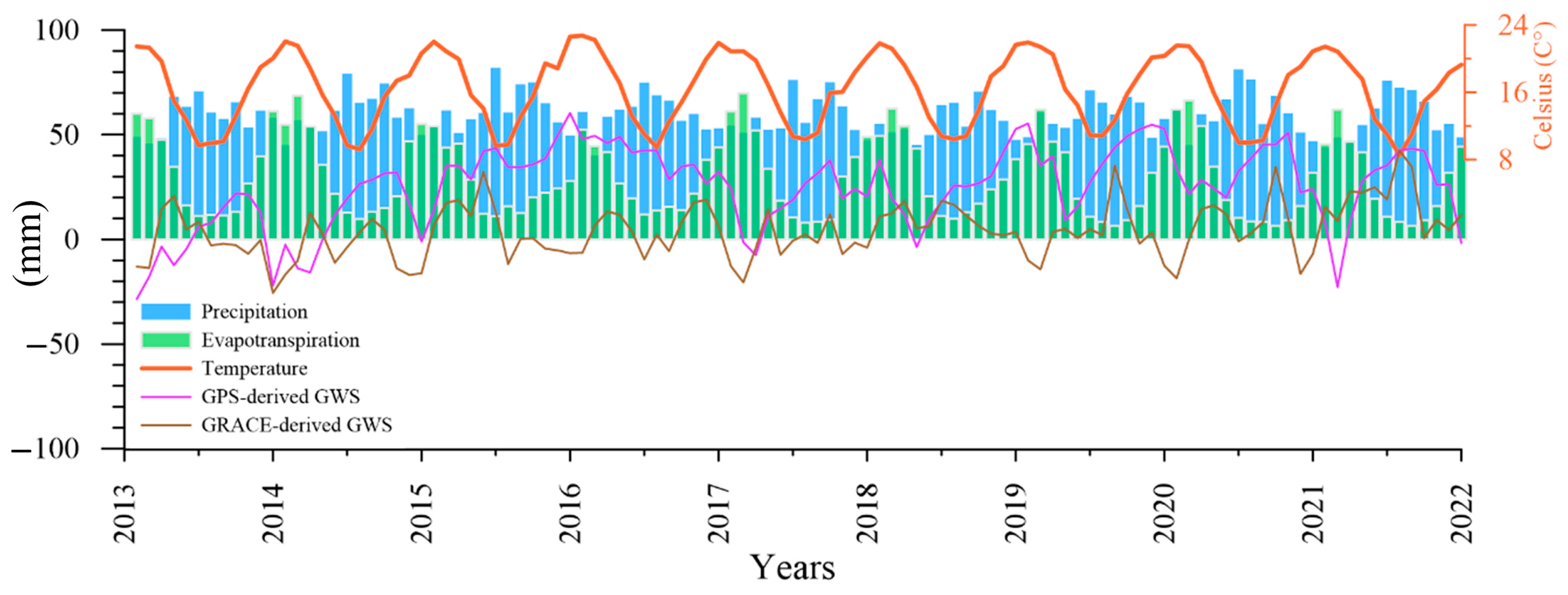
5.1.2. Climate
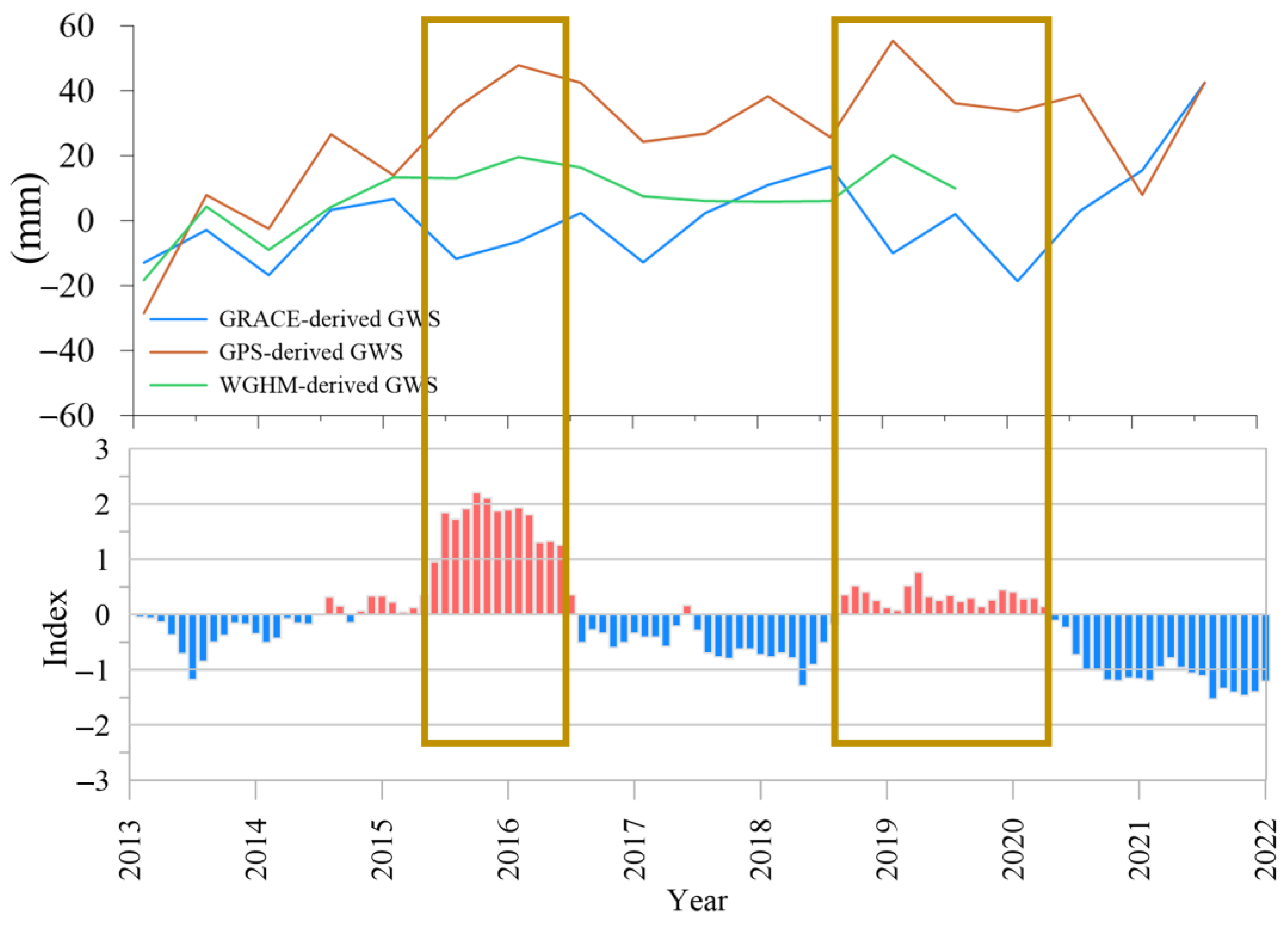
5.1.3. Groundwater Storage and ENSO
6. Conclusions
Author Contributions
Funding
Data Availability Statement
Acknowledgments
Conflicts of Interest
References
- El Kharraz, J.; El-Sadek, A.; Ghaffour, N.; Mino, E. Water scarcity and drought in WANA countries. Procedia Eng. 2012, 33, 14–29. [Google Scholar] [CrossRef]
- Chaudhari, S.; Pokhrel, Y.; Moran, E.; Miguez-Macho, G. Multi-decadal hydrologic change and variability in the Amazon River basin: Understanding terrestrial water storage variations and drought characteristics. Hydrol. Earth Syst. Sci. 2019, 23, 2841–2862. [Google Scholar] [CrossRef]
- Syed, T.H.; Famiglietti, J.S.; Rodell, M.; Chen, J.; Wilson, C.R. Analysis of terrestrial water storage changes from GRACE and GLDAS. Water Resour. Res. 2008, 44, W02433. [Google Scholar] [CrossRef]
- Baalousha, H. Assessment of a groundwater quality monitoring network using vulnerability mapping and geostatistics: A case study from Heretaunga Plains, New Zealand. Agric. Water Manag. 2010, 97, 240–246. [Google Scholar] [CrossRef]
- Cázares Escareño, J.; Júnez-Ferreira, H.E.; González-Trinidad, J.; Bautista-Capetillo, C.; Robles Rovelo, C.O. Design of Groundwater Level Monitoring Networks for Maximum Data Acquisition at Minimum Travel Cost. Water 2022, 14, 1209. [Google Scholar] [CrossRef]
- Osman, A.I.A.; Ahmed, A.N.; Chow, M.F.; Huang, Y.F.; El-Shafie, A. Extreme gradient boosting (Xgboost) model to predict the groundwater levels in Selangor Malaysia. Ain Shams Eng. J. 2021, 12, 1545–1556. [Google Scholar] [CrossRef]
- Osman, A.I.A.; Ahmed, A.N.; Huang, Y.F.; Kumar, P.; Birima, A.H.; Sherif, M.; Sefelnasr, A.; Ebraheemand, A.A.; El-Shafie, A. Past, Present and Perspective Methodology for Groundwater Modeling-Based Machine Learning Approaches. Arch. Comput. Methods Eng. 2022, 29, 3843–3859. [Google Scholar] [CrossRef]
- Strassberg, G.; Scanlon, B.R.; Rodell, M. Comparison of seasonal terrestrial water storage variations from GRACE with groundwater-level measurements from the High Plains Aquifer (USA). Geophys. Res. Lett. 2007, 34, L14402. [Google Scholar] [CrossRef]
- Xie, X.; Xu, C.; Wen, Y.; Li, W. Monitoring groundwater storage changes in the Loess Plateau using GRACE satellite gravity data, hydrological models and coal mining data. Remote Sens. 2018, 10, 605. [Google Scholar] [CrossRef]
- Barbosa, S.A.; Pulla, S.T.; Williams, G.P.; Jones, N.L.; Mamane, B.; Sanchez, J.L. Evaluating Groundwater Storage Change and Recharge Using GRACE Data: A Case Study of Aquifers in Niger, West Africa. Remote Sens. 2022, 14, 1532. [Google Scholar] [CrossRef]
- Jin, S.; Feng, G. Large-scale variations of global groundwater from satellite gravimetry and hydrological models, 2002–2012. Glob. Planet. Chang. 2013, 106, 20–30. [Google Scholar] [CrossRef]
- Croteau, M.; Nerem, R.; Loomis, B.; Sabaka, T. Development of a daily GRACE mascon solution for terrestrial water storage. J. Geophys. Res. Solid Earth 2020, 125, e2019JB018468. [Google Scholar] [CrossRef]
- Wang, L.; Chen, C.; Du, J.; Wang, T. Detecting seasonal and long-term vertical displacement in the North China Plain using GRACE and GPS. Hydrol. Earth Syst. Sci. 2017, 21, 2905–2922. [Google Scholar] [CrossRef]
- Lenczuk, A.; Klos, A.; Bogusz, J. Studying spatio-temporal patterns of vertical displacements caused by groundwater mass changes observed with GPS. Remote Sens. Environ. 2023, 292, 113597. [Google Scholar] [CrossRef]
- Bagheri-Gavkosh, M.; Hosseini, S.M.; Ataie-Ashtiani, B.; Sohani, Y.; Ebrahimian, H.; Morovat, F.; Ashrafi, S. Land subsidence: A global challenge. Sci. Total Environ. 2021, 778, 146193. [Google Scholar] [CrossRef]
- Xi, R.; Liang, Y.; Chen, Q.; Jiang, W.; Chen, Y.; Liu, S. Analysis of annual deformation characteristics of Xilongchi dam using historical GPS observations. Remote Sens. 2022, 14, 4018. [Google Scholar] [CrossRef]
- Tan, W.; Dong, D.; Chen, J.; Wu, B. Analysis of systematic differences from GPS-measured and GRACE-modeled deformation in Central Valley, California. Adv. Space Res. 2016, 57, 19–29. [Google Scholar] [CrossRef]
- Liu, R.; Zou, R.; Li, J.; Zhang, C.; Zhao, B.; Zhang, Y. Vertical displacements driven by groundwater storage changes in the North China Plain detected by GPS observations. Remote Sens. 2018, 10, 259. [Google Scholar] [CrossRef]
- Larochelle, S.; Chanard, K.; Fleitout, L.; Fortin, J.; Gualandi, A.; Longuevergne, L.; Rebischung, P.; Violette, S.; Avouac, J.p. Understanding the geodetic signature of large aquifer systems: Example of the Ozark Plateaus in central United States. J. Geophys. Res. Solid Earth 2022, 127, e2021JB023097. [Google Scholar] [CrossRef]
- Jiang, Z.; Hsu, Y.-J.; Yuan, L.; Feng, W.; Yang, X.; Tang, M. GNSS2TWS: An open-source MATLAB-based tool for inferring daily terrestrial water storage changes using GNSS vertical data. GPS Solut. 2022, 26, 1–7. [Google Scholar] [CrossRef]
- Argus, D.F.; Fu, Y.; Landerer, F.W. Seasonal variation in total water storage in California inferred from GPS observations of vertical land motion. Geophys. Res. Lett. 2014, 41, 1971–1980. [Google Scholar] [CrossRef]
- Knappe, E.; Bendick, R.; Martens, H.; Argus, D.; Gardner, W. Downscaling vertical GPS observations to derive watershed-scale hydrologic loading in the northern Rockies. Water Resour. Res. 2019, 55, 391–401. [Google Scholar] [CrossRef]
- De Vries, J.; Von Hoyer, M. Groundwater recharge studies in semi-arid Botswana—A review. In Estimation of Natural Groundwater Recharge; NATO ASI Series; Springer: Dordrecht, The Netherlands, 1988; Volume 222, pp. 339–347. [Google Scholar] [CrossRef]
- Fu, Y.; Argus, D.F.; Landerer, F.W. GPS as an independent measurement to estimate terrestrial water storage variations in Washington and Oregon. J. Geophys. Res. Solid Earth 2015, 120, 552–566. [Google Scholar] [CrossRef]
- Chew, C.C.; Small, E.E. Terrestrial water storage response to the 2012 drought estimated from GPS vertical position anomalies. Geophys. Res. Lett. 2014, 41, 6145–6151. [Google Scholar] [CrossRef]
- Jiang, Z.; Hsu, Y.-J.; Yuan, L.; Huang, D. Monitoring time-varying terrestrial water storage changes using daily GNSS measurements in Yunnan, southwest China. Remote Sens. Environ. 2021, 254, 112249. [Google Scholar] [CrossRef]
- Li, W.; Dong, J.; Wang, W.; Wen, H.; Liu, H.; Guo, Q.; Yao, G.; Zhang, C. Regional Crustal Vertical Deformation Driven by Terrestrial Water Load Depending on CORS Network and Environmental Loading Data: A Case Study of Southeast Zhejiang. Sensors 2021, 21, 7699. [Google Scholar] [CrossRef]
- Klos, A.; Dobslaw, H.; Dill, R.; Bogusz, J. Identifying the sensitivity of GPS to non-tidal loadings at various time resolutions: Examining vertical displacements from continental Eurasia. GPS Solut. 2021, 25, 89. [Google Scholar] [CrossRef]
- Gobron, K.; Rebischung, P.; Van Camp, M.; Demoulin, A.; de Viron, O. Influence of Aperiodic Non-Tidal Atmospheric and Oceanic Loading Deformations on the Stochastic Properties of Global GNSS Vertical Land Motion Time Series. J. Geophys. Res. Solid Earth 2021, 126, e2021JB022370. [Google Scholar] [CrossRef]
- Chanard, K.; Fleitout, L.; Calais, E.; Rebischung, P.; Avouac, J.P. Toward a global horizontal and vertical elastic load deformation model derived from GRACE and GNSS station position time series. J. Geophys. Res. Solid Earth 2018, 123, 3225–3237. [Google Scholar] [CrossRef]
- Sun, Z.; Long, D.; Yang, W.; Li, X.; Pan, Y. Reconstruction of GRACE data on changes in total water storage over the global land surface and 60 basins. Water Resour. Res. 2020, 56, e2019WR026250. [Google Scholar] [CrossRef]
- Pu, L.; Fan, D.; You, W.; Jiang, Z.; Yang, X.; Wan, X.; Nigatu, Z.M. Analysis of mass flux variations in the southern Tibetan Plateau based on an improved spatial domain filtering approach for GRACE/GRACE-FO solutions. Int. J. Remote Sens. 2022, 43, 3563–3591. [Google Scholar] [CrossRef]
- Scanlon, B.R.; Zhang, Z.; Save, H.; Wiese, D.N.; Landerer, F.W.; Long, D.; Longuevergne, L.; Chen, J. Global evaluation of new GRACE mascon products for hydrologic applications. Water Resour. Res. 2016, 52, 9412–9429. [Google Scholar] [CrossRef]
- Landerer, F.W.; Swenson, S. Accuracy of scaled GRACE terrestrial water storage estimates. Water Resour. Res. 2012, 48, 1–11. [Google Scholar] [CrossRef]
- Rodell, M.; Houser, P.; Jambor, U.; Gottschalck, J.; Mitchell, K.; Meng, C.-J.; Arsenault, K.; Cosgrove, B.; Radakovich, J.; Bosilovich, M. The global land data assimilation system. Bull. Am. Meteorol. Soc. 2004, 85, 381–394. [Google Scholar] [CrossRef]
- Singh, A.K.; Jasrotia, A.S.; Taloor, A.K.; Kotlia, B.S.; Kumar, V.; Roy, S.; Ray, P.K.C.; Singh, K.K.; Singh, A.K.; Sharma, A.K. Estimation of quantitative measures of total water storage variation from GRACE and GLDAS-NOAH satellites using geospatial technology. Quat. Int. 2017, 444, 191–200. [Google Scholar] [CrossRef]
- Ouma, Y.O.; Aballa, D.; Marinda, D.; Tateishi, R.; Hahn, M. Use of GRACE time-variable data and GLDAS-LSM for estimating groundwater storage variability at small basin scales: A case study of the Nzoia River Basin. Int. J. Remote Sens. 2015, 36, 5707–5736. [Google Scholar] [CrossRef]
- Amiri, V.; Ali, S.; Sohrabi, N. Estimating the Spatiotemporal of GRACE/GRACE-FO derived groundwater storage and depletion and validation with in-situ measurements of water level and quality (Yazd Province, Central Iran). J. Hydrol. 2023, 620, 129416. [Google Scholar] [CrossRef]
- Chen, Y.; Yang, K.; Qin, J.; Zhao, L.; Tang, W.; Han, M. Evaluation of AMSR-E retrievals and GLDAS simulations against observations of a soil moisture network on the central Tibetan Plateau. J. Geophys. Res. Atmos. 2013, 118, 4466–4475. [Google Scholar] [CrossRef]
- Yang, S.; Zeng, J.; Fan, W.; Cui, Y. Evaluating Root-zone Soil Moisture Products from GLEAM, GLDAS, and ERA5 based on in Situ ObServations and Triple Collocation Method Over the Tibetan Plateau. J. Hydrometeorol. 2022, 23, 1861–1878. [Google Scholar] [CrossRef]
- Fang, H.; Beaudoing, H.K.; Teng, W.L.; Vollmer, B.E. Global Land data assimilation system (GLDAS) products, services and application from NASA hydrology data and information services center (HDISC). In Proceedings of the ASPRS 2009 Annual Conference, Baltimore, MD, USA, 9–13 March 2009. [Google Scholar]
- Döll, P.; Fiedler, K. Global-scale modeling of groundwater recharge. Hydrol. Earth Syst. Sci. 2008, 12, 863–885. [Google Scholar] [CrossRef]
- Efon, E.; Ngongang, R.D.; Meukaleuni, C.; Wandjie, B.; Zebaze, S.; Lenouo, A.; Valipour, M. Monthly, Seasonal, and Annual Variations of Precipitation and Runoff Over West and Central Africa Using Remote Sens. and Climate Reanalysis. Earth Syst. Environ. 2022, 7, 67–82. [Google Scholar] [CrossRef]
- Gu, G.; Adler, R.F. Observed variability and trends in global precipitation during 1979–2020. Clim. Dyn. 2022, 61, 131–150. [Google Scholar] [CrossRef]
- Ropelewski, C.; Janowiak, J.; Halpert, M. The climate Anomaly Monitoring System (CAMS); CAMS: Chennai, India, 1984. [Google Scholar]
- Vose, R.S.; Schmoyer, R.L.; Steurer, P.M.; Peterson, T.C.; Heim, R.; Karl, T.R.; Eischeid, J.K. The Global Historical Climatology Network: Long-Term Monthly Temperature, Precipitation, Sea Level Pressure, and Station Pressure data; Carbon Dioxide Information; Oak Ridge National Lab.: Oak Ridge, TN, USA, 1992. [Google Scholar]
- Fan, Y.; Van den Dool, H. A global monthly land surface air temperature analysis for 1948–present. J. Geophys. Res. Atmos. 2008, 113, 01103. [Google Scholar] [CrossRef]
- Ratnam, J.; Doi, T.; Richter, I.; Oettli, P.; Nonaka, M.; Behera, S. Using Selected Members of a Large Ensemble to Improve Prediction of Surface Air Temperature Anomalies Over Japan in the Winter Months From Mid-Autumn. Front. Clim. 2022, 4, 919084. [Google Scholar] [CrossRef]
- Dill, R.; Dobslaw, H. Numerical simulations of global-scale high-resolution hydrological crustal deformations. J. Geophys. Res. Solid Earth 2013, 118, 5008–5017. [Google Scholar] [CrossRef]
- Farrell, W. Deformation of the Earth by surface loads. Rev. Geophys. 1972, 10, 761–797. [Google Scholar] [CrossRef]
- Longman, I. A Green’s function for determining the deformation of the Earth under surface mass loads: 2. Computations and numerical results. J. Geophys. Res. 1963, 68, 485–496. [Google Scholar] [CrossRef]
- Lai, Y.R.; Wang, L.; Bevis, M.; Fok, H.S.; Alanazi, A. Truncated singular value decomposition regularization for estimating terrestrial water storage changes using GPS: A case study over Taiwan. Remote Sens. 2020, 12, 3861. [Google Scholar] [CrossRef]
- Dziewonski, A.M.; Anderson, D.L. Preliminary reference Earth model. Phys. Earth Planet. Inter. 1981, 25, 297–356. [Google Scholar] [CrossRef]
- Matthews, M.V.; Segall, P. Estimation of depth-dependent fault slip from measured surface deformation with application to the 1906 San Francisco earthquake. J. Geophys. Res. Solid Earth 1993, 98, 12153–12163. [Google Scholar] [CrossRef]
- Pan, Y.; Ding, H.; Li, J.; Shum, C.; Mallick, R.; Jiao, J.; Li, M.; Zhang, Y. Transient hydrology-induced elastic deformation and land subsidence in Australia constrained by contemporary geodetic measurements. Earth Planet. Sci. Lett. 2022, 588, 117556. [Google Scholar] [CrossRef]
- Li, J.; Wang, S.; Zhou, F. Time series analysis of long-term terrestrial water storage over Canada from GRACE satellites using principal component analysis. Can. J. Remote Sens. 2016, 42, 161–170. [Google Scholar] [CrossRef]
- Awange, J.L.; Gebremichael, M.; Forootan, E.; Wakbulcho, G.; Anyah, R.; Ferreira, V.G.; Alemayehu, T. Characterization of Ethiopian mega hydrogeological regimes using GRACE, TRMM and GLDAS datasets. Adv. Water Resour. 2014, 74, 64–78. [Google Scholar] [CrossRef]
- He, M.; Shen, W.; Jiao, J.; Pan, Y. The Interannual Fluctuations in Mass Changes and Hydrological Elasticity on the Tibetan Plateau from Geodetic Measurements. Remote Sens. 2021, 13, 4277. [Google Scholar] [CrossRef]
- Lloyd-Hughes, B.; Saunders, M.A. A drought climatology for Europe. Int. J. Climatol. A J. R. Meteorol. Soc. 2002, 22, 1571–1592. [Google Scholar] [CrossRef]


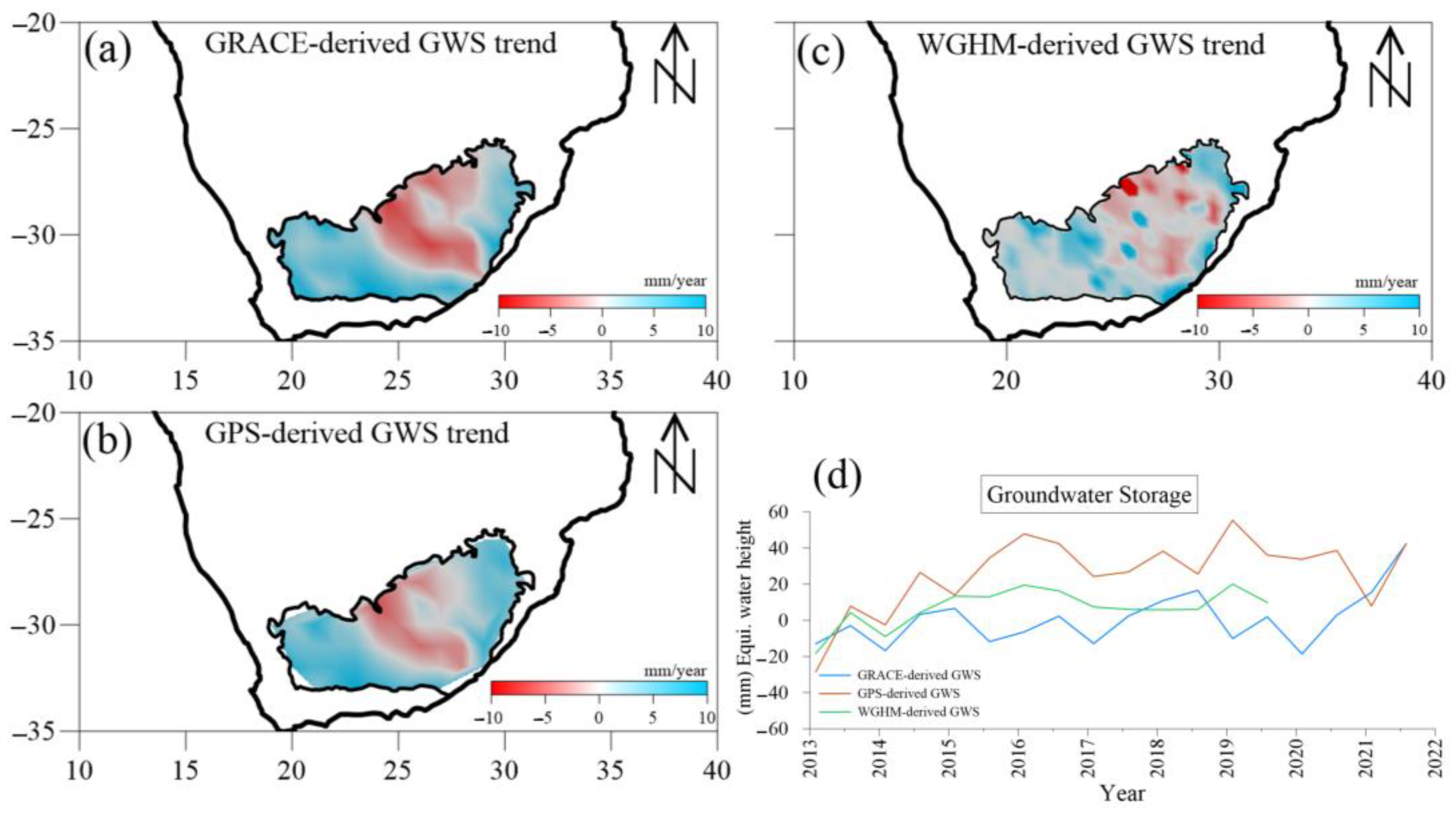
| GWS | GWS Trend (mm/Year) | |
|---|---|---|
| 2013–2019 | 2013–2021 | |
| GPS-derived GWS | 2.37 ± 0.09 | 2.59 ± 0.12 |
| GRACE-derived GWS | 1.52 ± 0.11 | 1.41 ± 0.08 |
| WGHM-derived GWS | 1.98 ± 0.08 | - |
| GWS | EOF-1 (%) | EOF-2 (%) |
|---|---|---|
| GPS-derived GWS | 71.83 | 28.17 |
| GRACE-derived GWS | 68.92 | 31.08 |
Disclaimer/Publisher’s Note: The statements, opinions and data contained in all publications are solely those of the individual author(s) and contributor(s) and not of MDPI and/or the editor(s). MDPI and/or the editor(s) disclaim responsibility for any injury to people or property resulting from any ideas, methods, instructions or products referred to in the content. |
© 2023 by the authors. Licensee MDPI, Basel, Switzerland. This article is an open access article distributed under the terms and conditions of the Creative Commons Attribution (CC BY) license (https://creativecommons.org/licenses/by/4.0/).
Share and Cite
Mohasseb, H.A.; Shen, W.; Jiao, J.; Wu, Q. Groundwater Storage Variations in the Main Karoo Aquifer Estimated Using GRACE and GPS. Water 2023, 15, 3675. https://doi.org/10.3390/w15203675
Mohasseb HA, Shen W, Jiao J, Wu Q. Groundwater Storage Variations in the Main Karoo Aquifer Estimated Using GRACE and GPS. Water. 2023; 15(20):3675. https://doi.org/10.3390/w15203675
Chicago/Turabian StyleMohasseb, Hussein A., Wenbin Shen, Jiashuang Jiao, and Qiwen Wu. 2023. "Groundwater Storage Variations in the Main Karoo Aquifer Estimated Using GRACE and GPS" Water 15, no. 20: 3675. https://doi.org/10.3390/w15203675