Article

Assessing the Impact of Climate and Land-Use Changes on the Hydrologic Cycle Using the SWAT Model in the Mun River Basin in Northeast Thailand

by
Dibesh Khadka
1,2,
Mukand S. Babel
1,2,* and
Ambili G. Kamalamma
1,3
1
Water Engineering and Management (WEM), School of Engineering and Technology (SET), Asian Institute of Technology (AIT), Pathum Thani 12120, Thailand
2
Centre for Water and Climate Adaptation Centre (CWCA), Asian Institute of Technology (AIT), Pathum Thani 12120, Thailand
3
Centre for Water Resources Development and Management (CWRDM), Kozhikode 673571, Kerala, India
*
Author to whom correspondence should be addressed.
Water 2023, 15(20), 3672; https://doi.org/10.3390/w15203672
Submission received: 30 August 2023 / Revised: 14 October 2023 / Accepted: 16 October 2023 / Published: 20 October 2023
(This article belongs to the Special Issue SWAT Modeling - New Approaches and Perspective)

Abstract

:
Climate change (CC) and land-use change (LUC) will alter a basin’s hydrological processes and water balance. Quantifying their significance is imperative in formulating appropriate countermeasures and management plans. This study assesses projected changes in hydrological variables under CC and LUC scenarios to provide multi-dimensional insight into water balance relevant to an agricultural watershed in Northeast Thailand. The soil and water assessment tool (SWAT) is utilized to simulate hydrological variables (evapotranspiration, soil moisture, surface runoff, and water yield) for the baseline (1981–2010) and the near-future (2021–2050) after calibrating the model. CC projections considering the CMIP6 model ensemble for the high-emission scenario (SSP5-8.5) show the annual rainfall may not change significantly (0.5% increase compared to baseline). However, the surface runoff will likely increase by 33% due to the projected increase in rainfall intensity and extremes. The increase in urban areas due to LUC for the business as usual (BAU) scenario is also expected to boost surface runoff by 38–87%. Similarly, the LUC scenario with forest expansion will increase evapotranspiration by up to 1.3%. While CC is anticipated to raise water yield by 11%, LUC may reduce it by 6%. Under the combined scenario, the yield is expected to increase by 8%, indicating CC as the dominating driver. The results show that although CC governs the runoff from the basin, land-use change will also impact flows at a monthly scale. Importantly, soil moisture in the future will decrease (8–9%) under both stressors, which will reverberate in the basin’s agricultural livelihood and socioeconomic settings unless the appropriate adaptation measures are implemented.

1. Introduction

Climate change and land-use change are the critical drivers that alter various hydrological processes [1,2,3,4,5]. Climate change impacts the water cycle by altering elements like precipitation, evapotranspiration, soil moisture, groundwater, and the scale and timing of runoff, while a land-use change can modify factors such as canopy interception, surface roughness, soil characteristics, albedo, etc., ultimately affecting evapotranspiration (ET), soil moisture (SM), and runoff [6,7]. Climate change has been perceived as the top global risk to humankind for the short and long term [8]. Almost all regions in the world have been experiencing the adverse manifestation of climate change in terms of extreme weather, floods, droughts, loss of biodiversity, etc. Human-induced global warming is set to transform the global climate structure, primarily by influencing the expansive atmospheric circulation that governs the movement of moisture and energy, changes in the large-scale hydrological cycles, and precipitation patterns, which will lead to an increased occurrence of floods and droughts [9,10]. Research shows climate change will enhance the dynamics of the hydrological cycle, increase the magnitude and frequency of extreme events, and redistribute water resources at various temporal and spatial scales in Southeast Asia [11].
Land-use change ranges from seasonal variation in the land cover characteristics and natural maturation of forest to long-term changes resulting from various human activities such as urbanization, deforestation, and conversion to agricultural lands and forest management practices [3]. Generally, forest covers have higher evapotranspiration demands and lower runoff than other land use such as urban areas, pastures, and agricultural land. On the other hand, urbanization drastically reduces the infiltration, and the runoff is enhanced in magnitude and timing [12].
Several hydrological modeling tools such as the soil and water assessment tool (SWAT), MIKE Système Hydrologique Européen (SHE), Precipitation-Runoff Modeling System (PRMS), Water Balance Simulation Model (WaSim)-ETH, and Hydrologiska Byråns Vattenbalansavdelning (HBV) have been developed and applied to various types of watersheds [13,14,15,16,17,18]. SWAT has been extensively used to assess the impacts of climate change and land-use change on hydrological variables [2,5,19,20,21]. SWAT is a conceptual, continuous, and semi-distributed hydrological model developed in the 1990s to assess the impacts of land use, management practices, and climate on water supplies [22,23]. Borah and Bera [24] compared 11 hydrological models and found that SWAT is more suitable for continuous simulations in agricultural watersheds. Under intermediate- and high-emission scenarios, Visweshwaran et al. [4] found that the rainfall, ET, soil moisture, and surface runoff will increase in the late century (2071–2100) in the Bharathapuzha River Basin, India. A study by Sharma et al. [25] using the SWAT model in the Dharoi catchment of the Sabarmati River Basin, India, found that climate change is the primary driver of the streamflow compared to land-use change. Similar findings were also reported by Iqbal et al. [26] in the source region of the Yellow River, China. Application of SWAT in the tropical watershed in Brazil by Lucas-Borja et al. [27] shows that the replacement of the forest with crops or pasture does not significantly impact the hydrological response. In contrast, complete deforestation would increase the surface runoff. Using SWAT, Son et al. [28] found in Northwest Vietnam that land-use change (deforestation and expansion of field crops and paddy) between 1992 and 2015 increased the ET by 1.8% whereas surface runoff decreased by 4.3%. Climate change has decreased ET (2.3%) and surface runoff (11.5%), mainly due to decreased rainfall. These studies show that the SWAT model can simulate hydrological processes under climate and land-use change scenarios. Integrating the crop growth module (Environmental Policy Integrated Climate—EPIC) within the SWAT has also enhanced its ability to reflect the impacts of land-use change on hydrology.
Other past studies of the impacts of climate change and land-use change on hydrology have mixed findings based on the geographical location of the study area. Under climate change, the annual average flow from the basin in southern Italy is projected to decrease by 20% in 2030–2059 [29]. Similar projections (28 to 52% decrease in flow in 2070–2100) are reported in a northern Spain catchment [30]. The Eerste River in South Africa will also observe a decrease in water availability by 8–18% by the end of the century [31]. In contrast, monsoon flow in the Chaliyar River Basin, India, is projected to increase by 8.1–25.4% in 2070–2099 [32]. Water yield is also projected to increase (25–82%) in the Taehwa River Watershed, Korea, in 2070–2100 [33]. Similarly, increases in annual flows under climate change are also reported in catchments in Nepal (in 2020–2059) [34]; Thailand (in 2071–2100) [35]; Southeast Asia (in 2075–2099) [36]; etc. Similarly, in a land-use change study in the Periyar River Watershed, India, Sadhwani et al. [12] shows that with the projected increase in the urban area (by 16.45%) and decrease in the plantation and forest area (13.7%), the runoff at the basin outlet might not be affected, but at the sub-basin level, the surface runoff will increase up to 56.6% by 2100. In the Bartin spring catchment located in northwestern Turkey, a land-use change scenario considering conversion of agricultural land to forest by 2026 shows an increase in evapotranspiration by 5% and a decrease in annual flow by 9%, while the reciprocal changes had an insignificant impact [3]. A study in the upper Bhima River Basin, India, shows that a scenario considering an increase in urban area by more than 5% has an evidential change in the runoff with an increase of 8–12% in highly urbanized sub-basins [37].
Studies have also explored the combined impacts of climate change and land-use change in basin runoff. The individual impacts of both drivers may vary temporally [7] and cannot be considered linearly cumulative [38]. In the Songkhram River Basin in Northeast Thailand, climate change significantly impacts flow more than land-use change [39]. Similar findings are also reported in North Carolina, USA [40]; Hoeya River Basin, Korea [41]; Neka River Basin, Iran [42]; Dongjiang River, China [43]; etc. A study in the Cahaba River in Alabama, USA, found that low flows are more sensitive to land-use change than climate change [44]. Although several studies have explored alteration in river flows due to individual and combined impacts of climate change and land-use change, few studies have estimated the impacts on other hydrological components such as evapotranspiration, soil moisture, etc. These are also critical hydrological variables, particularly for agriculture-dominated watersheds, which can considerably affect crop productivity. Our primary hypothesis is that both climate change and land-use change have significant impacts not only on the streamflow but also on evapotranspiration and soil moisture. By assessing these hydrological variables, we aim to provide multi-dimensional insights into hydrological water balance due to these two stressors in Northeast Thailand in the near future. To the authors’ knowledge, this research is the first of its kind in the region and employs a comprehensive water balance hydrological model to dissect various components. The study’s findings help formulate measures to tackle climate change and devise land-use plans for sustainable agriculture management in the basin.

2. Materials and Methods
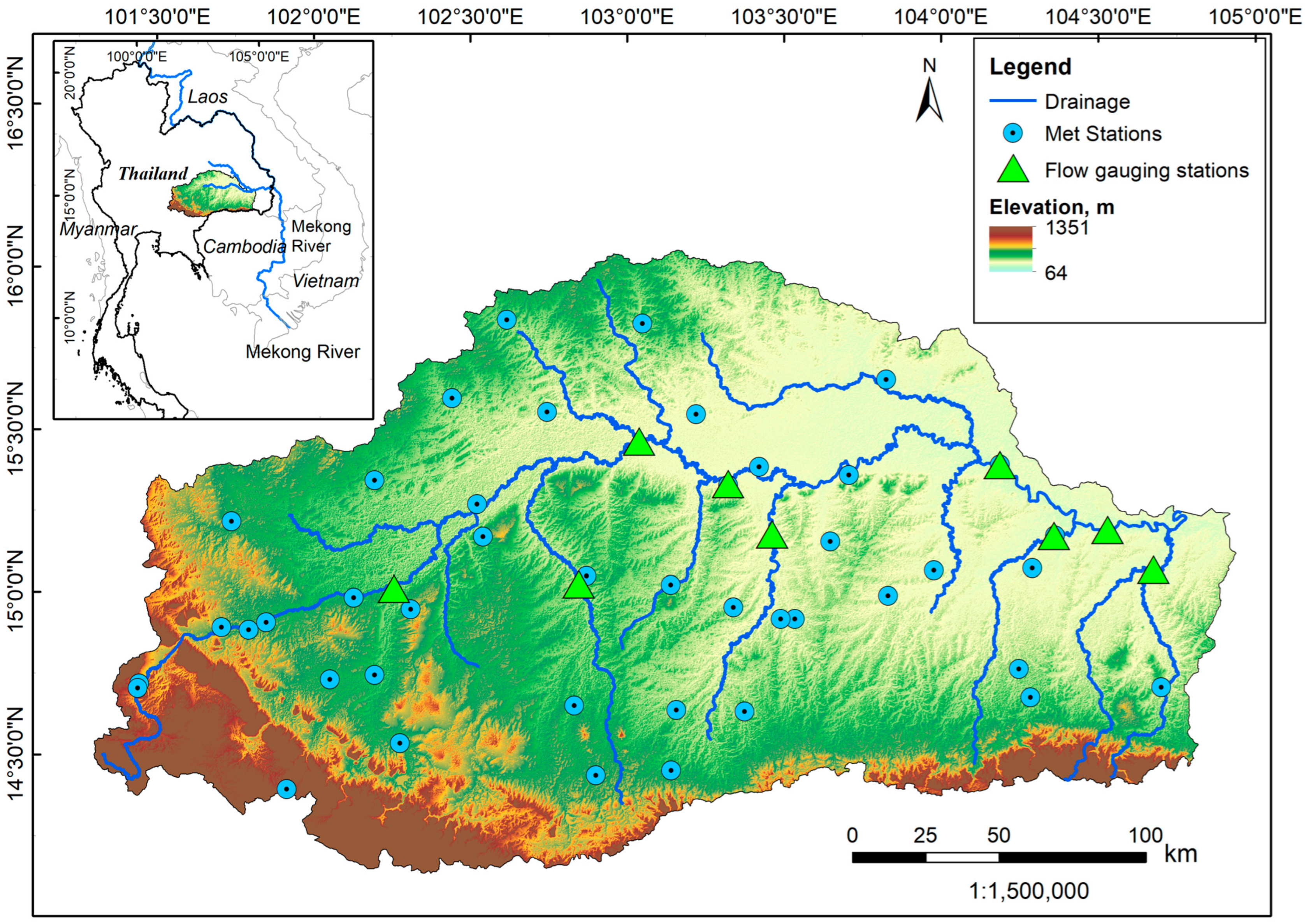
2.1. Study Area

Located in the Korat plateau in Northeast Thailand (Figure 1), the study area of the Mun River has an agriculture-dominated catchment where about 75% of the area is under cultivation. It is one of the major sub-basins of the Mekong River. The basin experiences a tropical climate and is heavily influenced by the southwest monsoonal system from the Indian Ocean. The annual average maximum and minimum temperatures vary spatially between 32.3 °C to 33.3 °C and 21.9 °C to 23.0 °C in the basin, while the annual rainfall has a distinct pattern showing increments from west to east in the basin (800 mm to 1700 mm) (Figure 2). June to October is the rainy season during which the southwest monsoon from the Indian Ocean brings 80% of the annual rainfall in the basin. From November to February, the northeast monsoon brings little or no rain in the basin. March to May is the pre-rainy and a transitional from the northeast to the southwest monsoon [45].
As shown in Figure 3, land use in the basin is dominated with agriculture, where rice is cultivated in about 55% of the entire area. Other major crops grown in the basin are cassava and sugarcane (sparsely distributed in the basin) and maize (mainly in the western part of the Nakhon Ratchasima province). Irrigation facilities reach only a fraction of the cultivation area in Northeast Thailand [46]. Most of the basin has sandy, loamy soil with a low fertility grade because of its limited ability to hold water and nutrients [47].

2.2. Data Used

2.2.1. Hydro-Meteorological Data

Observed rainfall data at 43 stations within the basin for 1981–2010 were utilized to generate gridded data at the spatial resolution of 0.25 degrees using the inverse distance weighting method [48]. The data are consistent with regional/global datasets (CPC, CHIRPS APHRODITE, etc.). As the observed temperature data are available in limited stations, data from the Climate Prediction Center (CPC) Global Land Surface Air Temperature Analysis [49], available at a 0.5-degree spatial resolution, were used. Within the basin, CPC data closely match observed station data with an average correlation coefficient above 0.95 and a root-mean-square error of about 0.8 °C [50]. Using spatially interpolated gridded climatic data has been found to improve streamflow simulation [51]. The daily river flow data (1996–2017) were collected from the Royal Irrigation Department (RID) of Thailand for nine gauging stations at the mainstream and tributaries of the Mun River Basin.
Future climate projections of daily maximum temperature, minimum temperature, and rainfall were acquired from Khadka et al. [48], who used eight climate models from the HighResMIPs [52] of Coupled Model Intercomparison Project phase 6 (CMIP6). Data are available for the near-future period (2021–2050) for the high-emission scenario of SSP5-8.5. The projection data were bias-corrected using the quantile mapping method. A study by Maneechot et al. [53] found that use of interpolation and bias correction of climate data improved their accuracy for extreme climate projections in the Chao Phraya River Basin, Thailand. Khadka et al. [48] found that compared to the baseline period (1981–2010), maximum and minimum temperatures are projected to increase by 1.29 °C and 1.37 °C, respectively, in the basin. Annual rainfall is projected to increase by 0.5% in the near-future; however, temporal variability will be higher with an increase in rainfall during the rainy season (by 2–8%) and a decrease in other months (by 6–11%). Details of the climate models from CMIP6 are provided in Table S1, and the spatial pattern of the projected climate in the near-future is presented in Figure S1.

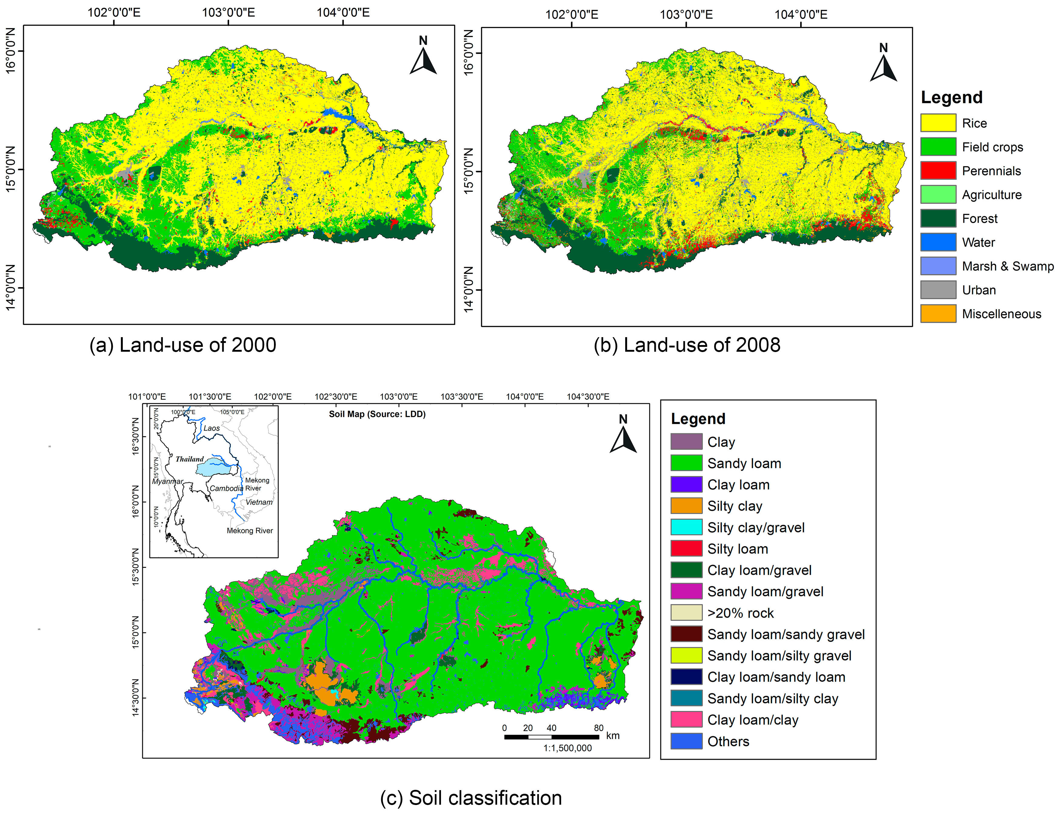
2.2.2. Land-Use and Soil Data
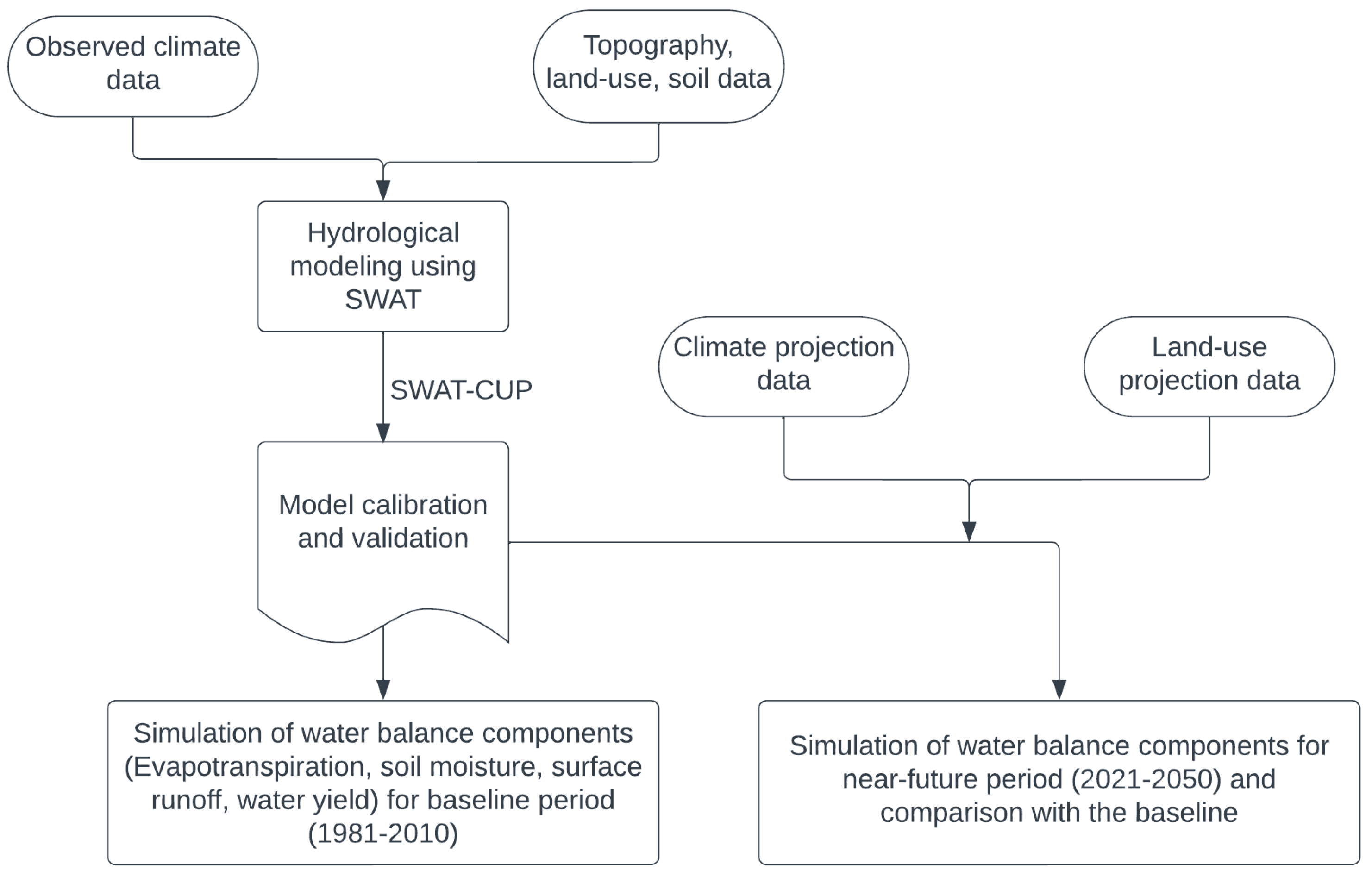
Land-use maps for 2000 and 2008 were acquired from Thailand’s Land Development Department (LDD). Table 1 shows that areas under rice and field crops (cassava, sugarcane, maize) decreased in 2008 while perennials and orchards, other agriculture (vegetables), and urban areas have increased. Forest occupies about slightly over 12% of areas during both years. The decreasing trend of rice fields is also attributable to the government’s crop diversification policy since the Seventh National Economic and Social Development Plan (NESDP), 1992–1996, to promote high-value and higher-value-added products [54]. Also, commercial crops like para rubber are expanding in Northeast Thailand with government support and economic reasons [55].
The future land use developed by Penny et al. [56] using the Future Land Use Simulation (FLUS) model is used in the study. Two scenarios, namely (i) business as usual (BAU) and (ii) combination of forest conservation and urban growth (CCU), are considered. The BAU scenario was developed based on past land-use trends between 2000 and 2017. CCU is a multi-objective scenario considering increased urban growth [57] and conservation [39]. Urban and forest extent were targeted at 12% and 25% of the total catchment area by 2060. Future land-use maps are available for 2025, 2035, and 2045, assuming each to represent a decade in the near-future. This integration of dynamic land-use change in hydrological simulation is found to be more accurate, particularly in the agricultural watershed [58]. Projected land use in the basin under both scenarios in 2045 is presented in Figure S2. Compared to 2008, rice fields are projected to decrease from 55.5% of the basin area to 45.6% under BAU and 39.3% under CCU. Similarly, the area under field crops will increase to 20.6% and 15.6% under BAU and CCU, respectively. Forest will be reduced to 11.2% under BAU, and an increase to 22.3% under CCU. Perennials and orchards will increase to about 7.5% under both scenarios and urban to 7.2% and 9.5% under BAU and CCU, respectively.

2.3. Methodology

The overall methodology of the study is presented in Figure 4. The details on the hydrological modeling and simulations under climate change and land-use change scenarios are presented in following sub-sections.

2.3.1. Hydrological Simulation Using the Soil and Water Assessment Tool (SWAT)

SWAT was chosen to simulate the basin’s hydrological components for the baseline and future period under climate and land-use change scenarios. It is a continuous water and sediment yield model, which operates at a daily time scale [59]. Hydrologic processes simulated with SWAT include canopy storage, surface runoff, infiltration, evapotranspiration, lateral flow, tile drainage, redistribution of water within the soil profile, consumptive use through pumping (if any), return flow, and recharge with seepage from surface water bodies, ponds, and tributary channels [13]. Researchers have extensively used SWAT for hydrological studies under climate change and land-use change drivers [60,61,62,63,64], and it has been found to be suitable for continuous simulation for agricultural watersheds [24]. Further details on SWAT can be found in Neitsch et al. [59].
In this study, the watershed is divided into 57 sub-watersheds based on the topography and location of the hydrological stations, which are further sub-divided into 1855 hydrologic response units (HRUs) comprising homogenous land-use, slope, and soil characteristics. The Penman–Monteith method [65] was used to estimate the potential evapotranspiration. The model was calibrated and validated at monthly temporal resolutions for flows at nine stations. The calibration was conducted using the land-use map of 2008 and for the period 2006–2017. Similarly, validation involved the land use of 2000 and the period 1996–2005. For some stations, data are unavailable for the validation period (i.e., before 2005). In such a case, those stations were used only for calibration.
Table 2 presents the drainage area of each gauging station along with the percentage of the area under different land use. Most of the catchment area for each drainage point is dominated with rice fields, followed by field crops and forest. The catchment at station M159 has the highest coverage with rice fields; station M2A has field crops; and station M176 has forest. Table 3 shows the projected changes in the land-use class at each station in the near-future period for BAU and CCU scenarios. Of the dominating land-use class, for both scenarios, rice fields are projected to decrease (highest for BAU), and field crops are projected to increase (highest for BAU). Forest area is projected to decrease under BAU and increase under CCU scenarios.
To better capture the water balance in the basin, the model was also calibrated for evapotranspiration (ET) and soil moisture. The simulated ET using the model was compared with the remote-sensing-based ET data acquired from the Global Land Evapotranspiration: the Amsterdam Model (GLEAM ET) [66]. The GLEAM model is driven by satellite-based observations on air temperature, precipitation, and surface soil moisture and is available from 2003 to 2015 at a spatial resolution of 0.25 degrees. The ET includes open-water and bare-soil evaporations, plant transpiration, and interception losses [67]. Since data have been available only since 2003, simulated ET was compared only for the calibration period.
Soil moisture (SM) data for the calibration were obtained from the Global Land Data Assimilation System (GLDAS) Noah Land Surface Model (LSM) [68]. It is a global terrestrial modeling system that uses ground and satellite observations [69]. The data have been available since 2000 at a spatial resolution of 0.25 degrees. Since rice, forest, and field crops are the significant land uses in the basin, ET and SM were compared from the corresponding HRUs in the selected sub-basin, which has most of these land uses with the observed data. Pearson’s correlation coefficient (r) was used to compare the simulated ET and soil moisture with the observation.
The model was calibrated using SWAT-CUP software with the Sequential Uncertainty Fitting (SUFI) algorithm [70]. Critical model parameters were identified with a sensitivity analysis and p-value. In addition to the Nash–Sutcliffe Efficiency (NSE), Coefficient of Determination (R2), and Percentage Biases (Pbias) [71], model performance in simulating flows was also assessed using the P-factor and R-factor [70]. The P-factor is the fraction of the observation data encapsulated using the uncertainty range, while the R-factor is the ratio of range width and standard deviation of the observed values [70,72]. For perfect simulation, the P-factor shall have a value of one while the R-factor will be zero.

2.3.2. Future Hydrological Simulation under Climate Change and Land-Use Change Scenarios

The calibrated SWAT model simulated the water balance components for the baseline (1981–2010) and the near-future (2021–2050) under climate change and land-use change scenarios. Specifically, five future cases (shown in Table 4) are considered, and the projected changes were assessed with respect to the baseline. The study focused on changes in rainfall, potential evapotranspiration, actual evapotranspiration, surface runoff, and water yield in the basin as they have relevance to agricultural activities.

3. Results and Discussion

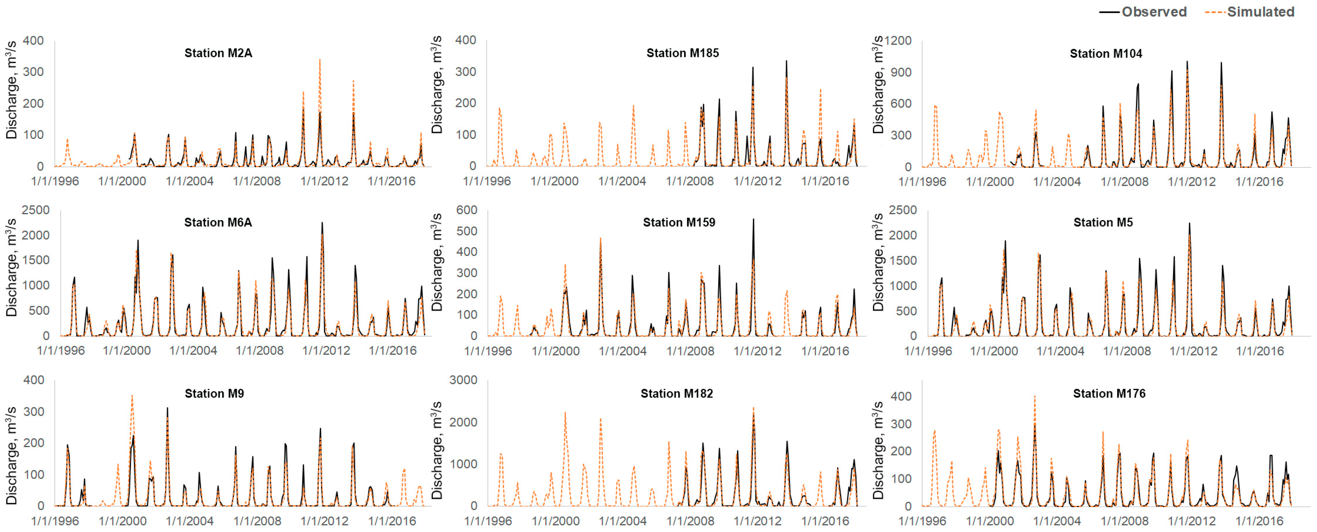
3.1. Calibration and Validation of SWAT

Based on the sensitivity analysis carried out in SWAT-CUP and the p-value of the parameters, thirteen parameters, as shown in Table 5, were chosen for calibrating the SWAT model. CN2.mgt, SOL_AWC.sol, GW_DELAY.gw, ESCO.hru, GWQMN.gw, and REVAPMN.gw are the most sensitive parameters with a p-value less than 0.05. In addition, other parameters are also found to be sensitive in some of the sub-basins in this study. The range of calibrated parameter values is well within the plausible limits (Table 5).
As indicated in Figure 1, simulated flows were calibrated at nine locations (indicated in Figure 1) and validated at six locations (due to lack of data) that cover the basin’s upper, middle, and lower parts. Statistical performance at each location is presented in Table 6. In many downstream stations, the P-factor exceeds 0.7 during the calibration and validation phases. At other stations, this factor is above 0.5. Except for station M182 (during calibration) and M6A (during validation), the R-factor for all other stations is below 1, indicating a limited uncertainty in the hydrological modeling. These values align with the recommendations given by Abbaspour et al. [70].
Furthermore, the R2 and NSE values at most stations range from 0.78 to 0.90 during calibration and 0.74 to 0.91 during validation. Except in three stations (M176, M9, and M2A) during validation, the P-biases are under 15%, indicating a strong alignment between the simulated and observed flows. As suggested by Abbaspour et al. [71], the performance of the SWAT model in these key statistics shows excellent simulation in most of the outlets. The results are similar to or better than previous studies [58,59,60] reported using SWAT in the region. Similarly, considering several calibration/validation locations ensures that the compensating errors within various sub-basins do not give a false impression of accuracy at the basin outlet. Visual representation of the calibration and validation of flow is presented in Figure 5, which shows that the model simulation captures the temporal pattern of the observed flow in all stations very well. Although some high flows at some sub-basins are underestimated, the model captures low flows very well, and this is a crucial trait required for hydrological simulation in an agricultural catchment [24]. In addition to uncertainties with the hydrological modeling, the discrepancies of simulated flow with observation could be due to inaccuracies in the conversion of point to areal average rainfall, measurements of high flows (which in most cases are extrapolated from the rating curves), etc.
The simulated values of ET and SM exhibit a commendable correlation with observations, as shown in Table 7. HRUs from twelve sub-basins, predominantly rice-cultivated, were compared with observations for evaluation. Similarly, HRUs from five forest-heavy sub-basins and three with field crops as the principal land use are considered. The correlation between observed and simulated ET is as follows: rice ranges from 0.68 to 0.78, forests from 0.57 to 0.75, and field crops from 0.30 to 0.57 during the calibration phase. The corresponding correlation coefficients for SM are 0.69–0.86 for rice, 0.74–0.87 for forests, and 0.46–0.58 for field crops. Chen et al. [73] also reported the correlation between SWAT-simulated and GLDAS soil moisture between 0.58 and 0.86 in the Luanhe River Basin, China. Similar to our findings, the forest area had the highest correlation coefficients. It is worth noting that field crops have correlation coefficient of 0.3 to 0.57 with the observed evapotranspiration and 0.33 to 0.58 with the observed soil moisture. This relatively low correlation can be attributed to the fact that field crops, comprised mainly of three different crops, namely maize, cassava, and sugarcane, have varying water needs and growing season lengths. In the SWAT model, all field crops are lumped together, and this generalization can impact performance. Moreover, since the observed data are derived from satellites, it is inherently subject to biases. Still, the results remain acceptable, as suggested using a study in the USA [74], where the correlation between the SWAT-simulated soil moisture and Normalized Difference Vegetative Index (NDVI) for agriculture was close to 0.6 and judged to be an acceptable simulation with the model.
Overall, the results suggest that the developed SWAT model is robust with reasonable accuracy in simulating the hydrological processes within the basin, considering the uncertainties associated with the parameterization of models and the underestimation of high flows at some stations.

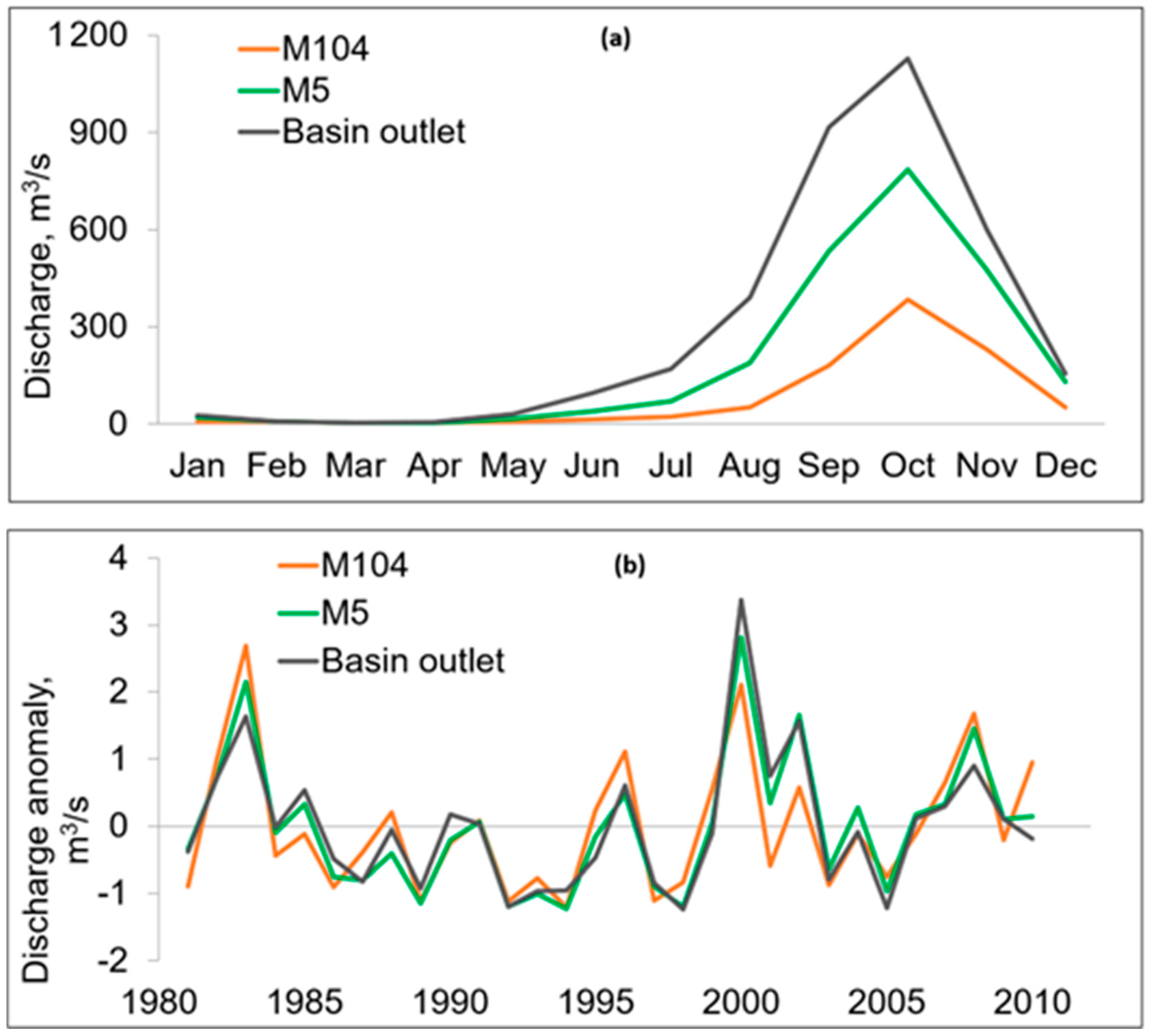
3.2. Baseline Simulation of Hydrological Components

The calibrated SWAT model was used to simulate the hydrological processes and outputs in the basin for the baseline period of 1981–2010. The summary of the most pertinent variables is shown in Table 8. The annual basin average rainfall during the observed period is about 1233 mm, of which about 80% is lost to evapotranspiration. High ET (989 mm annually) in the basin is due to significant agricultural fields and forest covers. The value is consistent with those reported by Giambelluca et al. [75] in the region. Similarly, the total recharge from the model is about 193 mm/year, which aligns with the findings from Lacombe et al. [76], who estimated it to be between 170 and 200 mm/year in the area.
Interestingly, the surface runoff constitutes only 22% of the water yield in the basin. As most of the basin has sandy loam soil, it facilitates more infiltration, resulting in less surface runoff and a higher proportion of sub-surface flow. The total annual water yield from the basin is 189 mm (about 16% of the rainfall). The major portion of the rainfall in the basin is lost as ET, which, in addition to climate, is also a function of soil types, slopes, and land use.
The monthly flow and annual cumulative flow data normalized using the long-term average and the standard deviation at three locations (Discharge anomaly = (Qi − Qm)/Standard deviation), namely at M104 (representing upper Mun), M5 (representing middle Mun), and at the basin outlet (lower Mun), are presented in Figure 6. Minimum flow in the basin occurs during March and April, while the higher flows are recorded during the rainy season, with maximum flow in October (about 1120 m3/s at the basin outlet). The annual average discharge at these three locations is 79 m3/s, 191 m3/s, and 301 m3/s, respectively. The anomaly plot (Figure 6b) also shows that most of the years between 1985 and 2000 are marked with low annual flows.

3.3. Projected Changes in Water Balance under Climate Change and Land-Use Change Scenarios

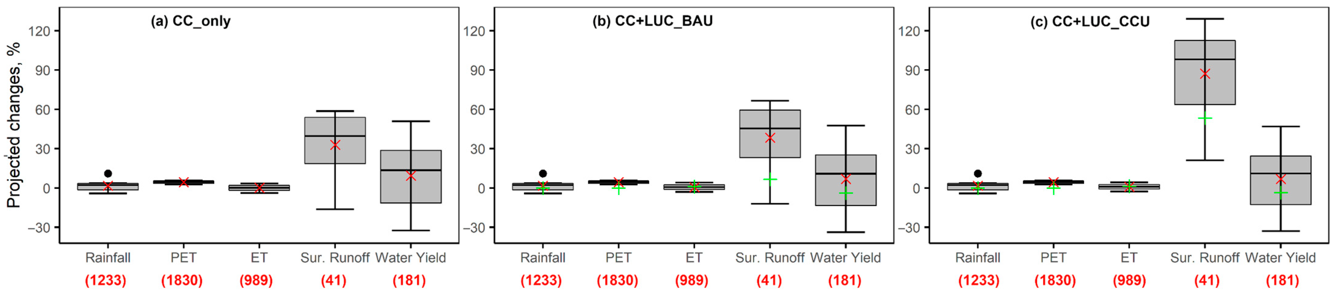
3.3.1. Water Balance Components

Projected changes in the water balance components (rainfall, potential evapotranspiration, actual evapotranspiration, surface runoff, and water yield) for individual and combined cases of climate change and land-use change scenarios are presented in Table 9 and Figure 7. Rainfall and PET are only affected by climate change (case1, case4, and case5), while actual ET, surface runoff, and water yield are affected by both drivers. The ensemble average annual rainfall during the near-future is projected to increase by less than a percent, although climate models projected changes from −5% to +10%. Similarly, PET is projected to rise by 4.4%, similar to estimates by Thompson et al. [77] in the basin, and is driven by an increase in future temperature. Under climate change, actual ET is also projected to increase slightly (0.2%) as it is affected by the increased ET demand. Notably, the increase in the actual ET is projected to be higher under both land-use change scenarios (by 1.0% and 1.3% under BAU and CCU, respectively). For both scenarios, the area under rice cultivation will decrease by 10% and 16% in the basin, while the area under field crops will increase by 6.3% and 1.3; the area under perennials and orchards will increase by 2.6% and 2.5%, respectively, for BAU and CCU. As field crops such as cassava, sugarcane, and perennials (rubber) have longer growing periods and water requirements [78], ET is expected to be higher. In addition, the CCU forest area is projected to grow from 12.5% to 22.3%, leading to enhanced evapotranspiration as reflected with a higher increase in ET than under the BAU scenario. Under the combined case of climate and land-use change, ET is projected to increase between 0.5 and 1.0% in the near-future.
As shown in Table 8, surface runoff during the baseline period is less than 5% of the total annual rainfall in the basin. Under climate change, it is projected to increase on average by 33% (13.2 mm). As the extreme rainfall and the rainfall intensity are projected to increase in the basin [48], it gives less opportunity for water to infiltrate the soil, thus increasing the proportion of surface runoff. Similarly, under the land-use change scenario, an increase in the surface runoff is predominantly affected by an increase in the urban area (7.2% in BAU and 9.5% in CCU of the basin area from 6.1% during baseline). With increased impervious areas, rainfall can quickly flow to the water channel. A case with climate change and land-use change in CCU will observe the highest increase in surface runoff by 87% (37 mm) because of the abovementioned reasons. Climate change will positively impact the annual water yield (+11%), while the land-use change will have the opposite effect, with decreased water yield by 5 and 6% for BAU and CCU, respectively. The decrease is mainly due to an increase in the ET in the near-future. A study by Yang et al. [35] in the Chao Phraya River, Thailand, reported that the future flows under climate change will increase by 10–20% in 2071–2100. The study’s findings also show that land-use change will decrease the flows by about 7% due to afforestation and a decrease in cropland. Liu et al. [20] also found that the expansion of forest and grassland will reduce the surface runoff, and an increase in cultivation land will increase the runoff. Similar results were also reported by Lucas-Borja et al. [27] in a tropical forest watershed. These results are very much aligned with the current findings. Under combined drivers, the yield will increase by about 8%. It is also noted from Figure 7 that the interquartile range (IQR) is exceptionally high for surface runoff and water yield. It is mainly because of the climate models’ high uncertainty associated with projected rainfall and the higher sensitivity of these variables to changes in rainfall.
Overall, the study suggests climate change will influence the hydrological responses more than the land-use change. The finding is supported with recent studies such as [35] in the Chao Phraya River Basin, Thailand; [39] in the Songkhram River Basin, Thailand; [28] in Nam Rom Basin, Vietnam; [79] in the Kabul River Basin, Afghanistan; [41] in the Hoeya River Basin, Korea; [42] in the Neka River Basin, Iran, etc. In addition, the impacts of climate change and land-use change are not cumulative, as suggested in [38,80], and vary temporally.

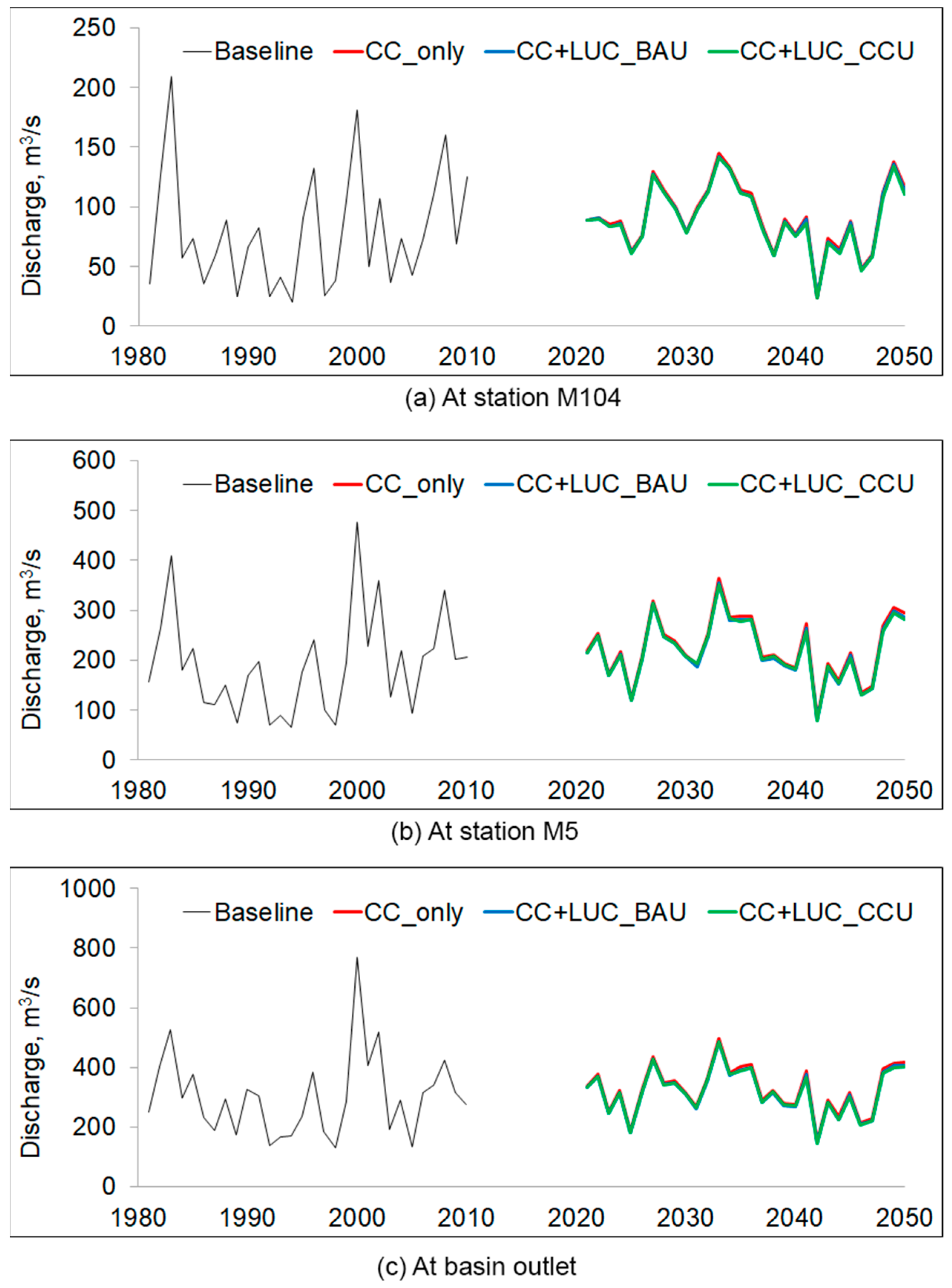
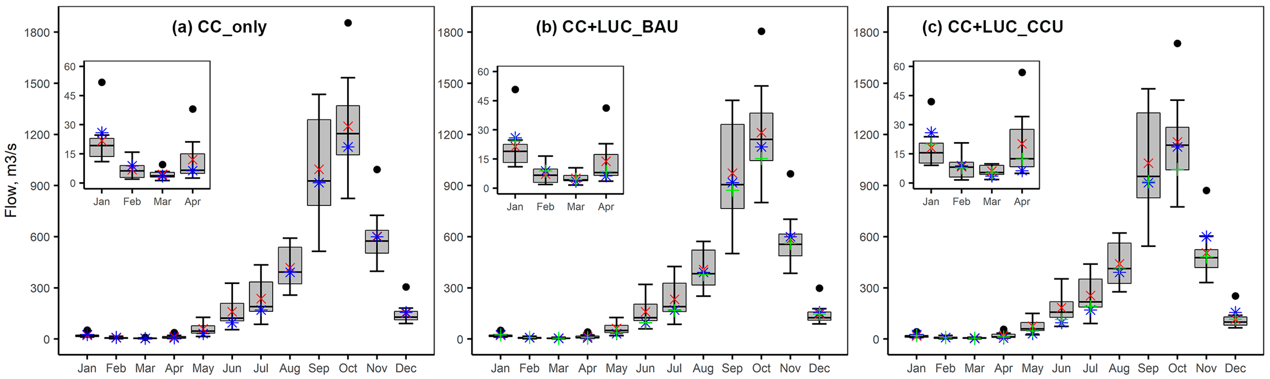
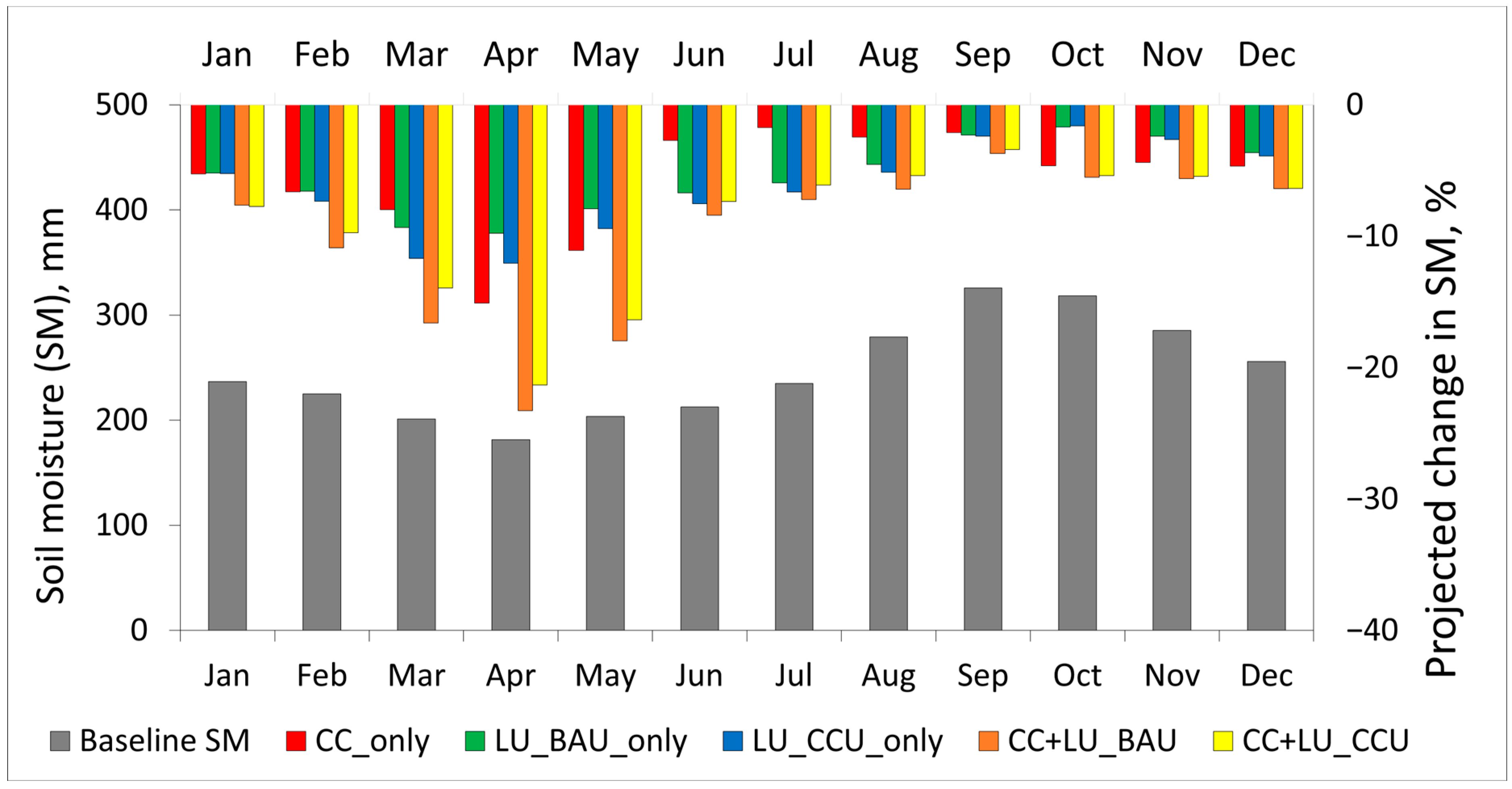
3.3.2. Projection of Flows and Soil Moisture

Figure 8 presents the projected annual average discharge at the outlet representing the upper part of Mun, the middle part, and the basin outlet for the near-future period. Cases considering climate change only and the combined case of climate change and land-use changes are analyzed. The figure clearly shows that the future discharge at all considered locations will be dominated with climate change. Land-use change (especially the CCU scenario) is expected to slightly decrease the flows in the future (5–6%). This is primarily because, under this scenario, forest area is expected to reach 25% of the total area by 2050. Consequently, the evapotranspiration demands in the future are expected to increase in most sub-basins, resulting in reduced flows. The climate change impacts the input variable (rainfall) of the hydrological cycle in addition to the hydrological process and other variables such as evapotranspiration, soil moisture, and surface runoff. While the land-use change will affect only the latter variables. This is one of the main reason climate change will have higher impacts in the future. Moreover, climate change affects the entire basin by increasing temperature and changing rainfall patterns, whereas land use can be localized.
The projected monthly flows in the near-future under climate change and land-use change scenarios are presented in Figure 9. Under climate change, the model ensemble suggests that the annual flow will increase by 10% while the increase during the wet season (May–October) is 14%. Similarly, under the land-use change scenario of BAU, the annual flow will decrease by 5%, and under CCU, it will decrease by 6%. Temporally, flows will increase during March–June by 5% under BAU while decreasing during August–January by 6%. The latter is more critical as it represents the majority of annual flow. Under CCU, flows will increase during March–August (13%) and decrease during September–February (16%). Under both drivers, flows are expected to increase from May to October, though the magnitudes are lesser than under climate change only. The results show that although the runoff from the basin is dominated with climate change, land-use change will also impact flows at a monthly scale.
It is also found that projected change in discharge under climate change is highly sensitive to changes in rainfall. For instance, the highest increase in the annual rainfall in the near-future period is projected with CNRM-CM6-1-HR (+10%), and the annual discharge will increase by 52–56% under combined drivers. Similarly, HadGEM3-GC31-HM projected the highest decrease in the annual rainfall (−5%), resulting in a decrease in discharge by 34–36%. This sensitivity of the discharge in the basin was also previously reported by Li and Fang [81], who used CMIP5 GCM and the SWAT model to simulate future flows. The rainfall–runoff ratio in the basin is projected to increase by 10% under climate change, mainly due to an increase in the surface runoff attributable to an increase in rainfall intensity and extremes.
The projected changes in the average soil moisture in the basin under the five cases considered are presented in Figure 10. There will be a reduction in soil moisture in all future cases. From February to May, the soil moisture decrease is highest while September to November is the lowest. Both climate change and land-use change are found to be essential drivers that affect future soil moisture, and their cumulative impacts are further aggravating. Climate change predominantly alters the timing and volume of surface water converting into soil moisture, while land-use change affects the timing and amount of evapotranspiration from the basin.
Consequently, the projected increase in the other water balance components (evapotranspiration and runoff) will adversely affect soil moisture. It will have severe implications in the basin as agriculture is the livelihood of the majority of the population in the basin. Reduced soil moisture will make future agricultural droughts more frequent and severe, affecting crop yields. It is especially crucial as only a fraction of the cultivation area has irrigation facilities. Thus, the impacts of climate change and land-use change will reverberate in the livelihood and socioeconomic settings of the region unless the appropriate adaptation measures are implemented.

4. Conclusions

The hydrological model SWAT is calibrated and validated for the Mun River Basin utilizing flow at nine gauging stations and satellite-based evapotranspiration and soil moisture. It is found that the surface runoff in the basin is very low (about 22% of the total flow), which is attributable to the soil type, slope, and the land use in the basin. The rainfall–runoff ratio is also low in the basin (0.11), mainly due to high evapotranspiration losses and low surface runoff generation. The southwest monsoon governs the monthly streamflow, where low flows are recorded during March and April and the highest flow is during October. In the near-future (2021–2050), PET will increase by 4.4%, while the ET will increase between 0.2 and 1.3%. The land-use change scenario for the combination of forest conservation and urban growth (CCU) has the highest increase in ET, mainly due to an increase in the forest area and perennial and field crops. Similarly, under the climate change scenario, surface runoff is projected to increase by 33% (13.2 mm), primarily because of increased rainfall extremes and intensity. The land-use change scenario considering CCU will also have an increased surface runoff by 49% (20 mm) by 2045 due to a projected increase in the urban area in the near future by 55% from the current extent. Under climate change, the water yield from the basin is expected to increase by 11%, while the land-use change for BAU and CCU will decrease by 5 and 6%, respectively. Under the combined drivers, the yields are expected to increase by 8% compared to the baseline.
Although significant efforts are made to calibrate and validate simulated flows, due to a lack of observed data, ET and SM are calibrated using global products, which are susceptible to inherited biases. Future projections can be more comprehensive, considering multiple SSPs and land-use scenarios to capture the range of uncertainties. Moreover, the study’s findings could be validated by replicating the study in other regions. As intricately related, climate change is also affected by land-use change and vice versa. The current study has not considered these dynamics of climate change and land-use change while projecting future water balance. Despite these limitations, the study shows the impacts of climate change will be higher than the land use in future streamflow, although they have opposite effects. Our study shows that climate change and land-use change will significantly affect soil moisture in the basin. This insight can be helpful for agricultural water management. The projected decrease in soil moisture in the near-future can significantly impact the agricultural activities in the basin, where most people rely on for their livelihood. Adaptation measures such as enhancing water use and various soil moisture conserving practices would be beneficial. In addition, reduced soil moisture will also have adverse impacts on the natural ecosystems by affecting plant growth, and biodiversity. It can also make forest susceptible to pests and diseases and increases the risk of wild fires. Similarly, the projected increase in surface runoff due to the expansion of urban areas will also pose challenges in stormwater management in the future. The study thus highlights that future policies should address climate change challenges and land-use change.

Supplementary Materials

The following supporting information can be downloaded at: https://www.mdpi.com/article/10.3390/w15203672/s1. Figure S1. Climate change projections for the near-future (2021–2050). The spatial pattern of the projected changes in (a) Tmax, (b) Tmin, and (c) rainfall for CMIP6 –SSP5-8.5 using the multi-model average for the near-future period. Changes are with respect to the baseline period. (Adopted from [48]). Figure S2. Land-use projections for the basin. (a) Projections under the Business as usual (BAU) scenario for 2050 and (b) Projection under the Combination of Forest Conservation and Urban Growth (CCU) scenario for 2050. (Adopted from [56]). Table S1. Details of climate models from HighResMIPs of CMIP6 considered in the study.

Author Contributions

Conceptualization, methodology, software, validation, formal analysis, data curation, writing—original draft preparation, D.K.; Conceptualization, writing—review and editing, supervision, funding acquisition, M.S.B.; Conceptualization, writing—review, A.G.K. All authors have read and agreed to the published version of the manuscript.

Funding

This research was funded by the National Research Council of Thailand (NRCT) (grant number: RDG6130025) and the Natural Environment Research Council (NERC) (grant number: NE/S002901/1) under the Newton Fund program.

Data Availability Statement

Data presented in the study will be made available upon request to the corresponding author.

Acknowledgments

We acknowledge funding agencies of the National Research Council of Thailand (NRCT) and the Natural Environment Research Council (NERC). We are also thankful to the Thai Meteorological Department (TMD), the Royal Irrigation Department (RID), and the Land Development Department (LDD) of Thailand for providing the necessary data.

Conflicts of Interest

The authors declare no conflict of interest.

References

  1. Jha, M.; Pan, Z.; Tackle, E.S.; Gu, R. Impacts of Climate Change on Streamflow in the Upper Mississippi River Basin: A Regional Climate Model Perspective. J. Geophys. Res. D Atmos. 2004, 109, D09105. [Google Scholar] [CrossRef]
  2. Osei, M.A.; Amekudzi, L.K.; Wemegah, D.D.; Preko, K.; Gyawu, E.S.; Obiri-Danso, K. The Impact of Climate and Land-Use Changes on the Hydrological Processes of Owabi Catchment from SWAT Analysis. J. Hydrol. Reg. Stud. 2019, 25, 100620. [Google Scholar] [CrossRef]
  3. Öztürk, M.; Copty, N.K.; Saysel, A.K. Modeling the Impact of Land Use Change on the Hydrology of a Rural Watershed. J. Hydrol. 2013, 497, 97–109. [Google Scholar] [CrossRef]
  4. Visweshwaran, R.; Ramsankaran, R.A.A.J.; Eldho, T.I.; Jha, M.K. Hydrological Impact Assessment of Future Climate Change on a Complex River Basin of Western Ghats, India. Water 2022, 14, 3571. [Google Scholar] [CrossRef]
  5. Brighenti, T.M.; Gassman, P.W.; Gutowski, W.J.; Thompson, J.R. Assessing the Influence of a Bias Correction Method on Future Climate Scenarios Using SWAT as an Impact Model Indicator. Water 2023, 15, 750. [Google Scholar] [CrossRef]
  6. Cuo, L.; Zhang, Y.; Gao, Y.; Hao, Z.; Cairang, L. The Impacts of Climate Change and Land Cover/Use Transition on the Hydrology in the Upper Yellow River Basin, China. J. Hydrol. 2013, 502, 37–52. [Google Scholar] [CrossRef]
  7. Wang, S.; Zhang, Z.; McVicar, T.R.; Guo, J.; Tang, Y.; Yao, A. Isolating the Impacts of Climate Change and Land Use Change on Decadal Streamflow Variation: Assessing Three Complementary Approaches. J. Hydrol. 2013, 507, 63–74. [Google Scholar] [CrossRef]
  8. World Economic Forum. The Global Risks Report 2023, 18th ed.; World Economic Forum: Geneva, Switzerland, 2023; ISBN 978-2-940631-36-0. [Google Scholar]
  9. Hartmann, D.L.B.T.-I.G. (Ed.) Chapter 6 Atmospheric General Circulation and Climate. In Global Physical Climatology; Academic Press: Cambridge, MA, USA, 1994; Volume 56, pp. 136–170. ISBN 0074-6142. [Google Scholar]
  10. Bates, B.C.; Kundzewicz, Z.W.; Wu, S.; Palutikof, J.P. (Eds.) Climate Change and Water. Technical Paper of the Intergovernmental Panel on Climate Change; IPCC Secretariat: Geneva, Switzerland, 2008; 210p. [Google Scholar]
  11. Chen, H.; Sun, J. Anthropogenic Warming Has Caused Hot Droughts More Frequently in China. J. Hydrol. 2017, 544, 306–318. [Google Scholar] [CrossRef]
  12. Sadhwani, K.; Eldho, T.I.; Jha, M.K.; Karmakar, S. Effects of Dynamic Land Use/Land Cover Change on Flow and Sediment Yield in a Monsoon-Dominated Tropical Watershed. Water 2022, 14, 3666. [Google Scholar] [CrossRef]
  13. Arnold, J.G.; Moriasi, D.N.; Gassman, P.W.; Abbaspour, K.C.; White, M.J.; Srinivasan, R.; Santhi, C.; Harmel, R.D.; Van Griensven, A.; Van Liew, M.W.; et al. SWAT: Model Use, Calibration, and Validation. Trans. ASABE 2012, 55, 1491–1508. [Google Scholar] [CrossRef]
  14. DHI MIKE SHE Volume 2: Reference Guide. Available online: https://manuals.mikepoweredbydhi.help/2017/Water_Resources/MIKE_SHE_Printed_V2.pd (accessed on 5 May 2020).
  15. Leavesley, G.H.; Lichty, R.W.; Troutman, B.M.; Saindon, L.G. Precipitation-Runoff Modeling System; User’s Manual; US Department of the Interior: Washington, DC, USA, 1983.
  16. Yira, Y.; Diekkrüger, B.; Steup, G.; Bossa, A.Y. Modeling Land Use Change Impacts on Water Resources in a Tropical West African Catchment (Dano, Burkina Faso). J. Hydrol. 2016, 537, 187–199. [Google Scholar] [CrossRef]
  17. Lindström, G.; Johansson, B.; Persson, M.; Gardelin, M.; Bergström, S. Development and Test of the Distributed HBV-96 Hydrological Model. J. Hydrol. 1997, 201, 272–288. [Google Scholar] [CrossRef]
  18. Usman, M.; Ndehedehe, C.E.; Farah, H.; Ahmad, B.; Wong, Y.; Adeyeri, O.E. Application of a Conceptual Hydrological Model for Streamflow Prediction Using Multi-Source Precipitation Products in a Semi-Arid River Basin. Water 2022, 14, 1260. [Google Scholar] [CrossRef]
  19. Reddy, N.N.; Reddy, K.V.; Vani, J.S.L.S.; Daggupati, P.; Srinivasan, R. Climate Change Impact Analysis on Watershed Using QSWAT. Spat. Inf. Res. 2018, 26, 253–259. [Google Scholar] [CrossRef]
  20. Liu, Y.; Xu, Y.; Zhao, Y.; Long, Y. Using SWAT Model to Assess the Impacts of Land Use and Climate Changes on Flood in the Upper Weihe River, China. Water 2022, 14, 2098. [Google Scholar] [CrossRef]
  21. Chen, C.; Gan, R.; Feng, D.; Yang, F.; Zuo, Q. Quantifying the Contribution of SWAT Modeling and CMIP6 Inputting to Streamflow Prediction Uncertainty under Climate Change. J. Clean. Prod. 2022, 364, 132675. [Google Scholar] [CrossRef]
  22. Arnold, J.G.; Srinivasan, R.; Muttiah, R.S.; Williams, J.R. Large Area Hydrologic Modeling And Assessment Part I: Model Development 1. JAWRA J. Am. Water Resour. Assoc. 1998, 34, 73–89. [Google Scholar] [CrossRef]
  23. Douglas-Mankin, K.R.; Srinivasan, R.; Arnold, J.G. Soil and Water Assessment Tool (SWAT) Model: Current Developments and Applications. Trans. ASABE 2010, 53, 1423–1431. [Google Scholar] [CrossRef]
  24. Borah, D.K.; Bera, M. Watershed-Scale Hydrologic And Nonpoint-Source Pollution Models: Review Of Applications. Trans. ASAE 2004, 47, 789–803. [Google Scholar] [CrossRef]
  25. Sharma, A.; Patel, P.L.; Sharma, P.J. Influence of Climate and Land-Use Changes on the Sensitivity of SWAT Model Parameters and Water Availability in a Semi-Arid River Basin. Catena 2022, 215, 106298. [Google Scholar] [CrossRef]
  26. Iqbal, M.; Wen, J.; Masood, M.; Masood, M.U.; Adnan, M. Impacts of Climate and Land-Use Changes on Hydrological Processes of the Source Region of Yellow River, China. Sustainability 2022, 14, 14908. [Google Scholar] [CrossRef]
  27. Lucas-Borja, M.E.; Carrà, B.G.; Nunes, J.P.; Bernard-Jannin, L.; Zema, D.A.; Zimbone, S.M. Impacts of Land-Use and Climate Changes on Surface Runoff in a Tropical Forest Watershed (Brazil). Hydrol. Sci. J. 2020, 65, 1956–1973. [Google Scholar] [CrossRef]
  28. Son, N.T.; Le Huong, H.; Loc, N.D.; Phuong, T.T. Application of SWAT Model to Assess Land Use Change and Climate Variability Impacts on Hydrology of Nam Rom Catchment in Northwestern Vietnam. Environ. Dev. Sustain. 2022, 24, 3091–3109. [Google Scholar] [CrossRef]
  29. De Girolamo, A.M.; Barca, E.; Leone, M.; Lo Porto, A. Impact of Long-Term Climate Change on Flow Regime in a Mediterranean Basin. J. Hydrol. Reg. Stud. 2022, 41, 101061. [Google Scholar] [CrossRef]
  30. Oduor, B.O.; Campo-Bescós, M.Á.; Lana-Renault, N.; Casalí, J. Effects of Climate Change on Streamflow and Nitrate Pollution in an Agricultural Mediterranean Watershed in Northern Spain. Agric. Water Manag. 2023, 285, 108378. [Google Scholar] [CrossRef]
  31. Du Plessis, J.A.; Kalima, S.G. Modelling the Impact of Climate Change on the Flow of the Eerste River in South Africa. Phys. Chem. Earth Parts A/B/C 2021, 124, 103025. [Google Scholar] [CrossRef]
  32. Ansa Thasneem, S.; Thampi, S.G.; Chithra, N.R. Uncertainties in Future Monsoon Flow Predictions in the Context of Projected Climate Change: A Study of the Chaliyar River Basin. Environ. Res. 2023, 222, 115301. [Google Scholar] [CrossRef]
  33. Jeon, D.J.; Ligaray, M.; Kim, M.; Kim, G.; Lee, G.; Pachepsky, Y.A.; Cha, D.-H.; Cho, K.H. Evaluating the Influence of Climate Change on the Fate and Transport of Fecal Coliform Bacteria Using the Modified SWAT Model. Sci. Total Environ. 2019, 658, 753–762. [Google Scholar] [CrossRef]
  34. Khadka, D.; Babel, M.S.; Shrestha, S.; Tripathi, N.K. Climate Change Impact on Glacier and Snow Melt and Runoff in Tamakoshi Basin in the Hindu Kush Himalayan (HKH) Region. J. Hydrol. 2014, 511, 49–60. [Google Scholar] [CrossRef]
  35. Yang, S.; Zhao, B.; Yang, D.; Wang, T.; Yang, Y.; Ma, T.; Santisirisomboon, J. Future Changes in Water Resources, Floods and Droughts under the Joint Impact of Climate and Land-Use Changes in the Chao Phraya Basin, Thailand. J. Hydrol. 2023, 620, 129454. [Google Scholar] [CrossRef]
  36. Trang, N.T.T.; Shrestha, S.; Shrestha, M.; Datta, A.; Kawasaki, A. Evaluating the Impacts of Climate and Land-Use Change on the Hydrology and Nutrient Yield in a Transboundary River Basin: A Case Study in the 3S River Basin (Sekong, Sesan, and Srepok). Sci. Total Environ. 2017, 576, 586–598. [Google Scholar] [CrossRef] [PubMed]
  37. Samal, D.R.; Gedam, S. Assessing the Impacts of Land Use and Land Cover Change on Water Resources in the Upper Bhima River Basin, India. Environ. Chall. 2021, 5, 100251. [Google Scholar] [CrossRef]
  38. El-Khoury, A.; Seidou, O.; Lapen, D.R.; Que, Z.; Mohammadian, M.; Sunohara, M.; Bahram, D. Combined Impacts of Future Climate and Land Use Changes on Discharge, Nitrogen and Phosphorus Loads for a Canadian River Basin. J. Environ. Manag. 2015, 151, 76–86. [Google Scholar] [CrossRef] [PubMed]
  39. Shrestha, S.; Bhatta, B.; Shrestha, M.; Shrestha, P.K.P.K. Integrated Assessment of the Climate and Landuse Change Impact on Hydrology and Water Quality in the Songkhram River Basin, Thailand. Sci. Total Environ. 2018, 643, 1610–1622. [Google Scholar] [CrossRef]
  40. Qi, S.; Sun, G.; Wang, Y.; Mcnulty, S.G.; Myers, J.A.M. Streamflow Response to Climate and Landuse Changes in a Coastal Watershed in North Carolina. Trans. ASABE 2009, 52, 739–749. [Google Scholar] [CrossRef]
  41. Kim, J.; Choi, J.; Choi, C.; Park, S. Impacts of Changes in Climate and Land Use/Land Cover under IPCC RCP Scenarios on Streamflow in the Hoeya River Basin, Korea. Sci. Total Environ. 2013, 452–453, 181–195. [Google Scholar] [CrossRef]
  42. Shooshtari, S.J.; Shayesteh, K.; Gholamalifard, M.; Azari, M.; Serrano-Notivoli, R.; López-Moreno, J.I. Impacts of Future Land Cover and Climate Change on the Water Balance in Northern Iran. Hydrol. Sci. J. 2017, 62, 2655–2673. [Google Scholar] [CrossRef]
  43. Jiang, J.; Wang, Z.; Lai, C.; Wu, X.; Chen, X. Climate and Landuse Change Enhance Spatio-Temporal Variability of Dongjiang River Flow and Ammonia Nitrogen. Sci. Total Environ. 2023, 867, 161483. [Google Scholar] [CrossRef]
  44. Dosdogru, F.; Kalin, L.; Wang, R.; Yen, H. Potential Impacts of Land Use/Cover and Climate Changes on Ecologically Relevant Flows. J. Hydrol. 2020, 584, 124654. [Google Scholar] [CrossRef]
  45. TMD the Climate of Thailand. Climatological Group, Meteorological Development Bureau, Meteorological Department. 2015. Available online: https://www.Tmd.Go.Th/En/Archive/Thailand_climate.Pdf (accessed on 16 November 2018).
  46. Prabnakorn, S.; Maskey, S.; Suryadi, F.X.; de Fraiture, C. Rice Yield in Response to Climate Trends and Drought Index in the Mun River Basin, Thailand. Sci. Total Environ. 2018, 621, 108–119. [Google Scholar] [CrossRef]
  47. Babel, M.S.; Agarwal, A.; Swain, D.K.; Herath, S. Evaluation of Climate Change Impacts and Adaptation Measures for Rice Cultivation in Northeast Thailand. Clim. Res. 2011, 46, 137–146. [Google Scholar] [CrossRef]
  48. Khadka, D.; Babel, M.S.; Collins, M.; Shrestha, S.; Virdis, S.G.P.P.; Chen, A.S. Projected Changes in the Near-Future Mean Climate and Extreme Climate Events in Northeast Thailand. Int. J. Climatol. 2022, 42, 2470–2492. [Google Scholar] [CrossRef]
  49. Fan, Y.; van den Dool, H. A Global Monthly Land Surface Air Temperature Analysis for 1948–Present. J. Geophys. Res. 2008, 113, D01103. [Google Scholar] [CrossRef]
  50. Khadka, D.; Babel, M.S.; Shrestha, S.; Virdis, S.G.P.; Collins, M. Multivariate and Multi-Temporal Analysis of Meteorological Drought in the Northeast of Thailand. Weather Clim. Extrem. 2021, 34, 100399. [Google Scholar] [CrossRef]
  51. Felix, M.L.; Jung, K. Impacts of Spatial Interpolation Methods on Daily Streamflow Predictions with SWAT. Water 2022, 14, 3340. [Google Scholar] [CrossRef]
  52. Haarsma, R.J.; Roberts, M.J.; Vidale, P.L.; Senior, C.A.; Bellucci, A.; Bao, Q.; Chang, P.; Corti, S.; Fučkar, N.S.; Guemas, V.; et al. High Resolution Model Intercomparison Project (HighResMIP~v1.0) for CMIP6. Geosci. Model Dev. 2016, 9, 4185–4208. [Google Scholar] [CrossRef]
  53. Maneechot, L.; Wong, Y.J.; Try, S.; Shimizu, Y.; Bharambe, K.P.; Hanittinan, P.; Ram-Indra, T.; Usman, M. Evaluating the Necessity of Post-Processing Techniques on D4PDF Data for Extreme Climate Assessment. Environ. Sci. Pollut. Res. 2023, 30, 102531–102546. [Google Scholar] [CrossRef]
  54. Kasem, S.; Thapa, G.B. Sustainable Development Policies and Achievements in the Context of the Agriculture Sector in Thailand. Sustain. Dev. 2012, 20, 98–114. [Google Scholar] [CrossRef]
  55. Wangpimool, W.; Pongput, K.; Tangtham, N.; Prachansri, S.; Gassman, P.W. The Impact of Para Rubber Expansion on Streamflow and Other Water Balance Components of the Nam Loei River Basin, Thailand. Water 2017, 9, 1. [Google Scholar] [CrossRef]
  56. Penny, J.; Djordjević, S.; Chen, A.S. Using Public Participation within Land Use Change Scenarios for Analysing Environmental and Socioeconomic Drivers. Environ. Res. Lett. 2021, 17, 025002. [Google Scholar] [CrossRef]
  57. Huang, Y.; Huang, J.L.; Liao, T.J.; Liang, X.; Tian, H. Simulating Urban Expansion and Its Impact on Functional Connectivity in the Three Gorges Reservoir Area. Sci. Total Environ. 2018, 643, 1553–1561. [Google Scholar] [CrossRef]
  58. Nepal, D.; Parajuli, P.B.; Ouyang, Y.; To, S.D.F.; Wijewardane, N. Assessing Hydrological and Water Quality Responses to Dynamic Landuse Change at Watershed Scale in Mississippi. J. Hydrol. 2023, 625, 129983. [Google Scholar] [CrossRef]
  59. Neitsch, S.L.; Arnold, J.G.; Kiniry, J.R.; Williams, J.R. Soil and Water Assessment Tool—Theoretical Documentation Version 2009. Texas Water Resources Institute, Texas A&M University. 2011. Available online: https://swat.tamu.edu/media/99192/swat2009-theory.pdf (accessed on 16 November 2018).
  60. Lin, B.; Chen, X.; Yao, H.; Chen, Y.; Liu, M.; Gao, L.; James, A. Analyses of Landuse Change Impacts on Catchment Runoff Using Different Time Indicators Based on SWAT Model. Ecol. Indic. 2015, 58, 55–63. [Google Scholar] [CrossRef]
  61. Zhou, F.; Xu, Y.; Chen, Y.; Xu, C.-Y.; Gao, Y.; Du, J. Hydrological Response to Urbanization at Different Spatio-Temporal Scales Simulated by Coupling of CLUE-S and the SWAT Model in the Yangtze River Delta Region. J. Hydrol. 2013, 485, 113–125. [Google Scholar] [CrossRef]
  62. Li, Z.; Liu, W.; Zhang, X.; Zheng, F. Impacts of Land Use Change and Climate Variability on Hydrology in an Agricultural Catchment on the Loess Plateau of China. J. Hydrol. 2009, 377, 35–42. [Google Scholar] [CrossRef]
  63. Fan, M.; Shibata, H. Simulation of Watershed Hydrology and Stream Water Quality under Land Use and Climate Change Scenarios in Teshio River Watershed, Northern Japan. Ecol. Indic. 2015, 50, 79–89. [Google Scholar] [CrossRef]
  64. Luo, M.; Liu, T.; Meng, F.; Duan, Y.; Bao, A.; Xing, W.; Feng, X.; De Maeyer, P.; Frankl, A. Identifying Climate Change Impacts on Water Resources in Xinjiang, China. Sci. Total Environ. 2019, 676, 613–626. [Google Scholar] [CrossRef]
  65. Allen, R.G.; Pereira, L.S.; Raes, D.; Smith, M. Crop Evapotranspiration: Guidelines for Computing Crop Water Requirements; FAO Irrigation and Drainage Paper 56; FAO: Rome, Italy, 1998. [Google Scholar]
  66. Martens, B.; Miralles, D.; Lievens, H.; van der Schalie, R.; de Jeu, R.; Férnandez-Prieto, D.; Beck, H.; Dorigo, W.; Verhoest, N. GLEAM v3: Satellite-Based Land Evaporation and Root-Zone Soil Moisture. Geosci. Model Dev. Discuss. 2016, 10, 1903–1925. [Google Scholar] [CrossRef]
  67. Miralles, D.G.; Holmes, T.R.H.; De Jeu, R.A.M.; Gash, J.H.; Meesters, A.G.C.A.; Dolman, A.J. Global Land-Surface Evaporation Estimated from Satellite-Based Observations. Hydrol. Earth Syst. Sci. 2011, 15, 453–469. [Google Scholar] [CrossRef]
  68. Rodell, M.; Houser, P.R.; Jambor, U.; Gottschalck, J.; Mitchell, K.; Meng, C.-J.; Arsenault, K.; Cosgrove, B.; Radakovich, J.; Bosilovich, M.; et al. The Global Land Data Assimilation System. Bull. Am. Meteorol. Soc. 2004, 85, 381–394. [Google Scholar] [CrossRef]
  69. Bi, H.; Ma, J.; Zheng, W.; Zeng, J. Comparison of Soil Moisture in GLDAS Model Simulations and in Situ Observations over the Tibetan Plateau. J. Geophys. Res. Atmos. 2016, 121, 2658–2678. [Google Scholar] [CrossRef]
  70. Abbaspour, K.C.; Rouholahnejad, E.; Vaghefi, S.; Srinivasan, R.; Yang, H.; Kløve, B. A Continental-Scale Hydrology and Water Quality Model for Europe: Calibration and Uncertainty of a High-Resolution Large-Scale SWAT Model. J. Hydrol. 2015, 524, 733–752. [Google Scholar] [CrossRef]
  71. Moriasi, D.N.; Arnold, J.G.; Van Liew, M.W.; Bingner, R.L.; Harmel, R.D.; Veith, T.L. Model Evaluation Guidelines for Systematic Quantification of Accuracy in Watershed Simulations. Trans. ASABE 2007, 50, 885–900. [Google Scholar] [CrossRef]
  72. Abbaspour, K.C.; Yang, J.; Maximov, I.; Siber, R.; Bogner, K.; Mieleitner, J.; Zobrist, J.; Srinivasan, R. Modelling Hydrology and Water Quality in the Pre-Alpine/Alpine Thur Watershed Using SWAT. J. Hydrol. 2007, 333, 413–430. [Google Scholar] [CrossRef]
  73. Chen, X.; Han, R.; Feng, P.; Wang, Y. Combined Effects of Predicted Climate and Land Use Changes on Future Hydrological Droughts in the Luanhe River Basin, China. Nat. Hazards 2022, 110, 1305–1337. [Google Scholar] [CrossRef]
  74. Narasimhan, B.; Srinivasan, R. Development and Evaluation of Soil Moisture Deficit Index (SMDI) and Evapotranspiration Deficit Index (ETDI) for Agricultural Drought Monitoring. Agric. For. Meteorol. 2005, 133, 69–88. [Google Scholar] [CrossRef]
  75. Giambelluca, T.W.; Mudd, R.G.; Liu, W.; Ziegler, A.D.; Kobayashi, N.; Kumagai, T.; Miyazawa, Y.; Lim, T.K.; Huang, M.; Fox, J.; et al. Evapotranspiration of Rubber (Hevea Brasiliensis) Cultivated at Two Plantation Sites in Southeast Asia. Water Resour. Res. 2016, 52, 660–679. [Google Scholar] [CrossRef]
  76. Lacombe, G.; Douangsavanh, S.; Vongphachanh, S.; Pavelic, P. Regional Assessment of Groundwater Recharge in the Lower Mekong Basin. Hydrology 2017, 4, 60. [Google Scholar] [CrossRef]
  77. Thompson, J.R.; Green, A.J.; Kingston, D.G. Potential Evapotranspiration-Related Uncertainty in Climate Change Impacts on River Flow: An Assessment for the Mekong River Basin. J. Hydrol. 2014, 510, 259–279. [Google Scholar] [CrossRef]
  78. Mangmeechai, A. Effects of Rubber Plantation Policy on Water Resources and Landuse Change in the Northeastern Region of Thailand. Geogr. Environ. Sustain. 2020, 13, 73–83. [Google Scholar] [CrossRef]
  79. Ougahi, J.H.; Karim, S.; Mahmood, S.A. Application of the SWAT Model to Assess Climate and Land Use/Cover Change Impacts on Water Balance Components of the Kabul River Basin, Afghanistan. J. Water Clim. Chang. 2022, 13, 3977–3999. [Google Scholar] [CrossRef]
  80. Tamm, O.; Maasikamäe, S.; Padari, A.; Tamm, T. Modelling the Effects of Land Use and Climate Change on the Water Resources in the Eastern Baltic Sea Region Using the SWAT Model. Catena 2018, 167, 78–89. [Google Scholar] [CrossRef]
  81. Li, C.; Fang, H. Assessment of Climate Change Impacts on the Streamflow for the Mun River in the Mekong Basin, Southeast Asia: Using SWAT Model. Catena 2021, 201, 105199. [Google Scholar] [CrossRef]
Figure 1. Location map of the Mun River Basin in Northeast Thailand showing topography, river lines, and hydro-meteorological stations.
Water 15 03672 g001
Figure 2. The spatial patterns of annual average (a) maximum temperature, (b) minimum temperature, and (c) rainfall of the basin during the baseline period (1981–2010).
Water 15 03672 g002
Figure 3. The spatial patterns of (a) land-use of 2000, (b) land-use of 2008, and (c) soil map of the basin. (Source: Land Development Department, Thailand).
Water 15 03672 g003
Figure 4. The methodological framework used in the study to assess projected changes in the water balance component in the near-future (2021–2050) under individual and combined impacts of climate change compared to the baseline (1981–2010).
Water 15 03672 g004
Figure 5. Comparison of SWAT-simulated flows with observations at nine locations during the period of calibration (2006–2017) and validation (1996–2005).
Water 15 03672 g005
Figure 6. Observed (a) monthly flows and (b) annual cumulative flow data normalized using the long-term average and the standard deviation at three locations corresponding to the upper, middle, and lower Mun River Basin for the baseline period (1981–2010).
Water 15 03672 g006
Figure 7. Projected changes in annual water balance for near-future period (2021–2050) with reference to baseline (1981–2010) considering future cases of climate change and land-use change scenarios. The boxplot shows the range of projections from eight climate models. The boxes represent the IQR with the horizontal line in the box corresponding to the median value and the whiskers to either the maximum/minimum values or 1.5 times the IQR. The red crosses are the values for the ensemble average, and the green plus sign is the value considering land use only. The absolute values of the variable (in mm) during the baseline period are presented within parenthesis ().
Water 15 03672 g007
Figure 8. Comparison of projected annual average flows in the near-future period for scenarios considering (i) climate change (CC_only), (ii) climate change and land-use change in BAU (CC+LUC_BAU), and climate change and land-use change in CCU (CC+LUC_CCU) with reference to baseline period at outlet of (a) upper Mun (M104), (b) middle Mun (M5), and (c) lower Mun (basin outlet).
Water 15 03672 g008
Figure 9. Boxplot shows the basin outlet’s monthly average flows using eight climate models for climate change and land-use change scenarios. The boxes represent the IQR with the horizontal line in the box corresponding to the median value and the whiskers to either the maximum/minimum values or 1.5 times the IQR. The red crosses are the values for the ensemble average, the green plus sign is the value considering land use only, and the blue stars are the values during the baseline period. Severities are shown as absolute values.
Water 15 03672 g009
Figure 10. Monthly average soil moisture (SM) during the baseline period (left axis) and the projected change in the monthly average soil moisture under five future cases considering climate change and land-use change compared to the baseline period (right axis).
Water 15 03672 g010
Table 1. Percentage of the basin area under various land uses in 2000 and 2008.
S.N.Land-Use Class% of the Basin Area
The Year 2000The Year 2008
1Rice60.2%55.5%
2Field Crop18.2%14.3%
3Perennials and Orchards (Rubber)1.7%4.9%
4Agriculture (Others)0.1%0.9%
5Forest12.2%12.5%
6Water Bodies1.5%2.7%
7Marsh and Swamp Land0.4%0.7%
8Urban4.8%6.1%
9Miscellaneous (Rangeland)0.9%2.5%
Table 2. Drainage area and percentage of land-use classes in the catchment of each hydrological station.
S.N.Hydrological Station IDDrainage Area (km2)% of Land-Use Class
RiceField CropPerennials and OrchardsAgriculture (Others)ForestWater BodiesMarsh and Swamp LandUrbanMiscellaneous
1M176298951.0%7.2%13.2%0.1%19.8%1.9%0.1%4.5%2.2%
2M2A313714.0%35.8%7.1%4.6%19.3%1.6%0.2%12.9%4.5%
3M9353066.6%5.1%3.9%0.1%13.8%1.8%0.1%5.9%2.7%
4M185461025.9%16.8%7.1%0.2%41.5%2.6%0.1%4.3%1.5%
5M159475469.6%3.9%6.4%0.3%7.5%2.7%0.1%7.9%1.6%
6M10424,64440.0%26.3%4.9%1.2%16.6%1.9%0.5%6.1%2.6%
7M6A28,01643.2%24.4%5.1%1.2%15.1%2.1%0.5%6.1%2.5%
8M544,32854.7%16.6%4.6%0.9%12.0%2.2%0.7%6.1%2.2%
9M18248,65855.9%15.5%4.5%0.9%12.0%2.2%0.7%6.1%2.3%
Table 3. Projected changes in the land-use class area in the near-future (2021–2050) compared to baseline (1981–2010) in the catchment of each hydrological station for business as usual (BAU) scenario. The projected changes for combination of forest conservation and urban growth (CCU) are shown in parenthesis.
S.N.Hydrological Station IDProjected Changes in the Land-Use
RiceField CropPerennials and OrchardsAgriculture (Others)ForestWater BodiesMarsh and Swamp LandUrbanMiscellaneous
1M176−16% (−30%)11% (2%)56% (20%)35% (36%)−9% (45%)38% (38%)8% (−27%)21% (63%)5% (−2%)
2M2A−41% (−23%)24% (−1%)−13% (−26%)−24% (−21%)−15% (12%)26% (26%)−3% (−27%)16% (26%)−12% (−1%)
3M9−14% (−23%)28% (−8%)213% (75%)48% (44%)−13% (61%)43% (43%)84% (58%)16% (62%)−14% (−18%)
4M185−26% (−34%)14% (−2%)73% (40%)−46% (−39%)−4% (11%)23% (23%)−49% (−56%)13% (37%)−26% (−28%)
5M159−21% (−35%)137% (57%)97% (43%)33% (46%)−4% (161%)41% (41%)−4% (−31%)25% (77%)12% (8%)
6M104−27% (−31%)34% (3%)36% (21%)−23% (−20%)−10% (42%)46% (45%)25% (2%)19% (45%)−3% (2%)
7M6A−27% (−32%)38% (5%)40% (20%)−26% (−22%)−11% (53%)45% (45%)21% (−2%)20% (49%)−2% (2%)
8M5−21% (−31%)42% (7%)73% (36%)−23% (−21%)−11% (80%)49% (49%)−13% (−40%)22% (60%)4% (6%)
9M182−20% (−30%)42% (7%)83% (39%)−20% (−19%)−11% (80%)48% (48%)−15% (−41%)21% (60%)3% (4%)
Table 4. Future cases considered for hydrological simulations for individual and combined climate change and land-use scenarios.
S.N.Future Cases
Case1Climate change only (CC_only)
Case2Land-use change under BAU (LU_BAU_only)
Case3Land-use change under CCU (LU_CCU_only)
Case4Climate change and land-use change under BAU (CC+LUC_BAU)
Case5Climate change and land-use change under CCU (CC+LUC_CCU)
Table 5. Parameters chosen for the calibration of the SWAT model, along with their initial and calibrated range.
S.N.ParameterDescriptionsInitial RangeCalibrated Range
MinMaxMinMax
1v__GW_DELAY.gwGroundwater delay time (days)0100240
2v__GWQMN.gwThreshold depth of water in the shallow aquifer required for return flow to occur (mm)015004751250
3v__GW_REVAP.gwGroundwater “revap” coefficient (-)0.020.20.0160.16
4v__REVAPMN.gwThreshold depth of water in the shallow aquifer for “revap” or percolation to the deep aquifer to occur (mm)0100300777
5v__RCHRG_DP.gwDeep aquifer percolation fraction (-)00.20.050.1
6v__CANMX.hruMaximum canopy storage (mm)020010
7v__ESCO.hruSoil evaporation compensation factor (-)010.640.94
8v__OV_N.hruManning’s “n” value for overland flow0.050.20.120.16
9v__CH_N2.rteManning’s “n” value for the main channel0.0140.10.0150.025
10v__CH_N1.subManning’s “n” value for the tributary channels0.0140.10.0150.025
11r__SOL_AWC.solAvailable water capacity in the soil layer (mm/mm soil)−0.250.250.10.2
12r__SOL_K().solSaturated hydraulic conductivity−0.250.2500.15
13r__CN2.mgtInitial SCS runoff curve number for moisture condition II (-)−0.150.15−0.16−0.07
Note: ‘v’ in the parameter name means absolute change where new values substitute the initial values in the SWAT database; ‘r’ in the parameter name means relative change where the initial values in the SWAT database are multiplied by factor 1 plus new values.
Table 6. Model performance in simulating monthly discharge during calibration and validation periods using statistical indicators.
OutletsCalibration (2006–2017)Validation (1996–2005)
P-FactorR-FactorR2NSEP-Bias (%)P-FactorR-FactorR2NSEP-Bias (%)
M50.820.970.860.859.10.861.090.840.83−1.4
M6A0.590.930.840.8412.00.771.320.830.78−11.7
M1760.720.560.870.865.40.460.630.910.74−29.6
M90.540.780.90.898.60.690.860.870.77−19.3
M1590.510.710.850.783.70.630.780.900.782.1
M2A0.560.830.810.785.10.50.900.850.7821.1
M1040.560.830.890.8711.3-----
M1820.821.080.840.835.0-----
M1850.440.830.790.78−0.5-----
Table 7. Range of Pearson’s correlation coefficients between simulated and observed evapotranspiration and soil moisture during the calibration and validation periods.
Hydrologic VariablesLand UseNumber of Sub-BasinsCalibrationValidation
EvapotranspirationRice120.68–0.78-
Forest50.57–0.75-
Field Crops30.30–0.57-
Soil moistureRice120.69–0.860.53–0.80
Forest50.74–0.870.59–0.79
Field Crops30.46–0.580.33–0.44
Table 8. Simulated variables for the baseline period using SWAT.
VariablesIn mm
Rainfall1233
PET1830
ET989
Total aquifer recharge193
Total groundwater storage48
Deep aquifer recharge10
Surface runoff, Q41
Total water yield189
Table 9. Average projected changes in the hydro-meteorological variables considering climate model ensemble for the near-future period (2021–2050) compared to the baseline period (1981–2010) for individual and combined cases of climate change (SSP5-8.5) and land-use change (BAU and CCU) scenarios.
S.N.Future CasesProjected Changes (%) in Near-Future Compared to the Baseline
RainfallPETETSurface RunoffWater Yield
1CC_only0.54.40.23311
2LU_BAU_only001.07−5
3LU_CCU_only001.349−6
4CC+LUC_BAU0.54.40.5388
5CC+LUC_CCU0.54.41.0878
Disclaimer/Publisher’s Note: The statements, opinions and data contained in all publications are solely those of the individual author(s) and contributor(s) and not of MDPI and/or the editor(s). MDPI and/or the editor(s) disclaim responsibility for any injury to people or property resulting from any ideas, methods, instructions or products referred to in the content.

