Article

Study on the Snowmelt Flood Model by Machine Learning Method in Xinjiang

1
Rivers, Lakes, Hydrology and Water Resources Center, Xinjiang Production and Construction Corps, Urumqi 830002, China
2
China Institute of Water Resource and Hydropower Research, Beijing 100038, China
3
Beijing Tianzhixiang Information Technology Co., Ltd., Beijing 100191, China
*
Author to whom correspondence should be addressed.
Water 2023, 15(20), 3620; https://doi.org/10.3390/w15203620
Submission received: 7 September 2023 / Revised: 27 September 2023 / Accepted: 11 October 2023 / Published: 16 October 2023
(This article belongs to the Special Issue Intelligent Modelling for Hydrology and Water Resources)

Abstract

:
There are many mountain torrent disasters caused by melting icebergs and snow in Xinjiang, which are very different from traditional mountain torrent disasters. Most of the areas affected by snowmelt are in areas without data, making it very difficult to predict and warn of disasters. Taking the Lianggoushan watershed at the southern foot of Boroconu Mountain as the research subject, the key factors were screened by Pearson correlation coefficient and the factor analysis method, and the data of rainfall, water level, temperature, air pressure, wind speed, and snow depth were used as inputs, respectively, with support vector regression (SVR), random forest (RF), k-nearest neighbor (KNN), artificial neural network (ANN), recurrent neural network (RNN), and long short-term memory neural network (LSTM) models used to simulate the daily average water level at the outlet of the watershed. The research results showed that the root mean square error (RMSE) values of SVR, RF, KNN, ANN, RNN, and LSTM in the training period were 0.033, 0.012, 0.016, 0.022, 0.011, and 0.010, respectively, and in the testing period they were 0.075, 0.072, 0.071, 0.075, 0.075, and 0.071, respectively. The performance of LSTM was better than that of other models, but it had more hyperparameters that needed to be optimized. The performance of RF was second only to LSTM; it had only one hyperparameter and was very easy to determine. The RF model showed that the simulation results mainly depended on the average wind speed and average sea level pressure data. The snowmelt model based on machine learning proposed in this study can be widely used in iceberg snowmelt warning and forecasting in ungauged areas, which is of great significance for the improvement of mountain flood prevention work in Xinjiang.

1. Introduction

The rivers and underlying surfaces in Xinjiang have poor permeability, and the ecological environment is extremely fragile. The extreme climate can easily cause natural disasters such as floods, mudslides, and landslides [1]. Xinjiang has 20,695 glaciers, which form a natural solid reservoir with an area of approximately 22,600 km2, accounting for 47.97% of China’s ice reserves [2]. The Tianshan Mountains straddle the entire territory of Xinjiang and are the birthplace of many international rivers. The cross-border rivers are complex and dense, and it is one of the areas with the most prominent cross-border river problems in the world, accounting for 20.0~40.0% of the total runoff in the Tianshan area [3]. Although snowmelt water is important for river runoff recharge, rapid snowmelt may also cause flood disasters. Snowmelt floods are often mixed with a large amount of ice, and may be accompanied by secondary disasters such as mudslides and landslides, causing great damage [4]. At the same time, due to the existence of seasonal frozen soil, the melting process of snow cover is uncertain, resulting in frequent occurrence of snowmelt floods in spring, which seriously threatens the safety of people’s lives and property [5].
The occurrence of extraordinary floods in Xinjiang is highly correlated with temperature and rainfall [6]. Huai and Muatta et al. used the SRM model to simulate snowmelt runoff based on factors such as rainfall, temperature, and snow area, and achieved relatively ideal results in areas without data in Xinjiang. At the same time, they pointed out that the SRM model is an empirical model and is very sensitive to temperature data. Insufficient temperature observation data limits the accuracy of the model [7,8]. Therefore, in recent years, using weather station observation data and satellite remote sensing products as input to drive the snowmelt runoff model to simulate the flood process has received widespread attention [9]. The SNTHERM (snow thermal) model [10] and the snowpack model [11] are multi-layer distributed snowmelt runoff models that can predict snow deposition, stratification, surface energy exchange, and mass balance, and can also predict the occurrence of avalanches. This type of model has physical meaning, but there are a large number of model parameters that need to be determined.
In recent years, the application of the machine learning algorithm snowmelt model has developed rapidly, playing an increasingly important role in hydrological simulation [12]. Vafakhah et al. used artificial neural network (ANN) and adaptive neural fuzzy inference systems (ANFIS) to simulate snowmelt runoff in Iran, and found that ANN and ANFIS had good performance in predicting snowmelt runoff [13]. Thapa developed a deep learning-based long-short-term memory (LSTM) network model for simulating the Himalayan Basin snowmelt-driven flow model, which uses remote sensing snow products as input and compares it with support vector regression (SVR) models, pointing out that LSTM is superior to SVR models [14]. Himan et al. drew an accurate flood susceptibility map for the Haraz watershed in Iran using a novel modeling approach (DBPGA) based on a deep belief network (DBN) with back propagation (BP) algorithm optimized by the genetic algorithm (GA) [15]. Wang et al. used RF and ANN to establish a runoff simulation model and pointed out that the snow data can effectively improve the accuracy of machine learning simulations of snowmelt runoff [16]. Yang et al. used the swin transformer model to evaluate the sensitivity of snowmelt in the Kunlun Mountains and found that altitude and distance from rivers are the most important factors affecting snowmelt floods in the study area [17]. Machine learning models are good at mining effective information from a large amount of basic data. The key of modeling is to determine reasonable hyperparameters.
Currently, meteorological indicators and hydrological models are widely used in Xinjiang to simulate snowmelt floods, and then to forecast and warn of flood disasters [18]. Flash floods usually occur in small and medium-sized catchments that lack of hydrological data, which are also main objects that need to be protected in flash flood prevention work. The purpose of this study is to explore a hydrological forecast method that can be used in practical work under limited data conditions. This time, the study was carried out on the Lianggoushan catchment of the southern slope of Mount Boroconu to analyze the internal relationship between data such as temperature, air pressure, wind speed, snow depth, rainfall, water level, etc., using support vector regression (SVR), random forest (RF), k-nearest neighbor (KNN), artificial neural network (ANN), recurrent neural network (RNN), and long short-term memory neural network (LSTM) models to simulate the daily average water level of the outlet section of the two valleys, optimize hyperparameters and compare the evaluation results of different models. The flood prediction model based on machine learning proposed in this paper can provide a reference and basis for flood forecasting and early warning work in Xinjiang.

2. Materials and Methods

2.1. Study Area

The Lianggoushan catchment is located in Nilek County, Xinjiang, at the southern foot of Mount Boroconu, with a water catchment area of 162 km2, a longest confluence path of 26 km, a maximum altitude of 4147 m, and a maximum drop of 2440 m. Figure 1 shows the geographical location of the Lianggoushan catchment. The Lianggoushan catchment has a temperate continental climate, which is characterized by long sunshine hours, large temperature differences between day and night, obvious vertical differences, abundant precipitation, short frost-free period, sharp temperature changes in spring, rapid cooling in autumn, and great disparity between winter and summer. The annual average temperature is 5.4 °C, the minimum temperature is −36.5 °C, and the maximum temperature is 37.1 °C; the average minimum temperature in January is less than −10 °C, which is a severe cold area. The annual average sunshine is 2795 h, and the annual average precipitation is 561.7 mm. The snow thickness is 34.7 cm, the average wind speed in the area is 2.9 m/s, and the wind direction is mainly northwest. The frost-free period is generally about 104 days, the depth of the seasonal frozen soil layer is generally about 0.9 m, and the maximum frozen soil depth is 1.0 m.

2.2. Data Collection

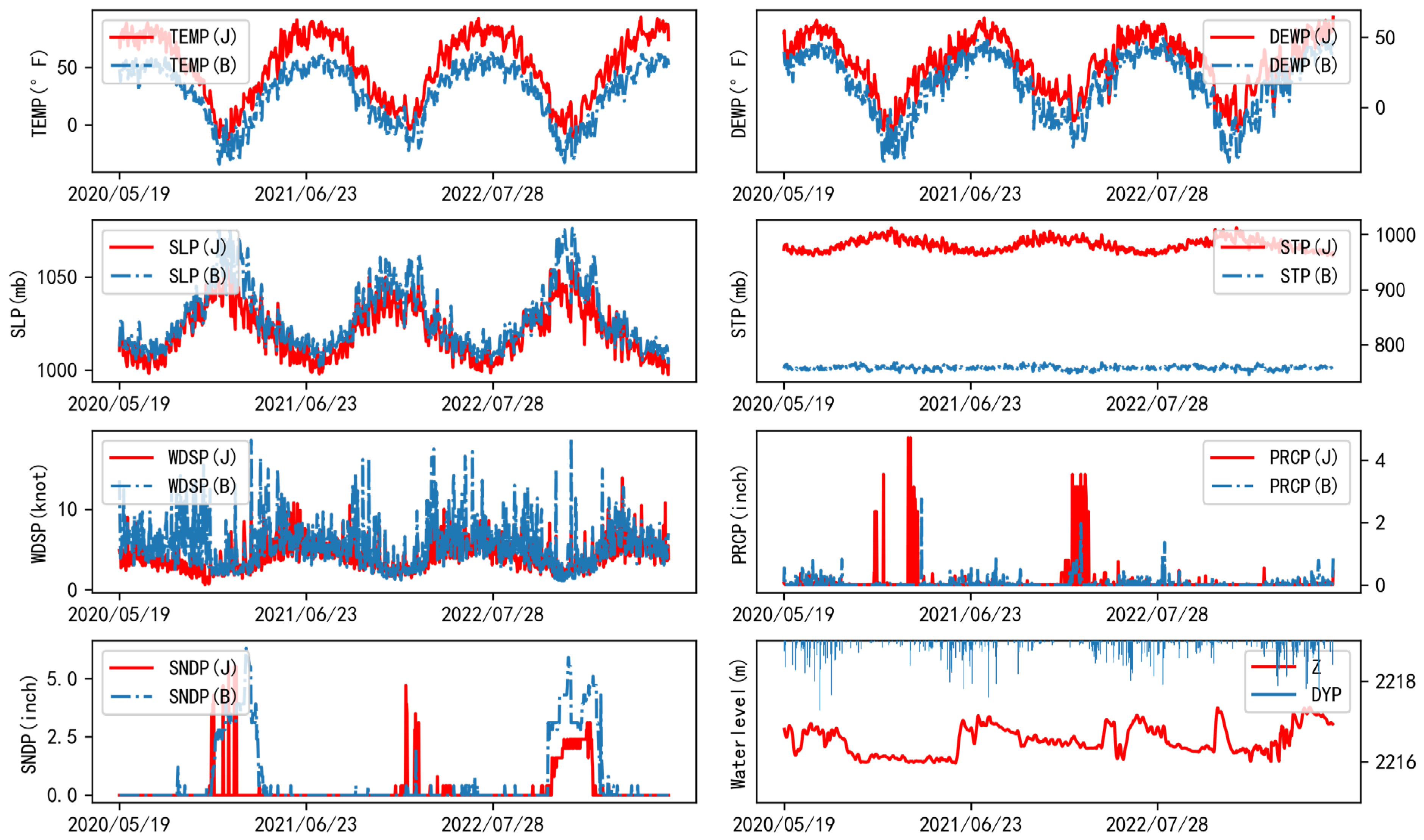
In this study, the stage and rainfall observation data of Lianggoushan Station from May 2020 to July 2023 were collected from the hydrological department of Xinjiang, and the daily precipitation data and daily average water level data were established after sorting out. Based on the GSOD meteorological dataset, the concurrent meteorological data of two meteorological stations (JINGHE and BAYANBULAK) near the Lianggoushan catchment were sorted out. The daily data of GSOD surface meteorological elements come from the USAF DATSAV3 surface data and the federal climate integrated surface hour (ISH) dataset. This time, the daily precipitation, average temperature, average dew point, average air pressure, average wind speed, maximum sustained wind speed, and snow cover depth, etc., in the dataset were used. The data items are shown in Table 1. Figure 2 shows the data collation results.
The dataset was divided into two parts during modeling, with data from May 2020 to December 2022 used for training the model and data from January 2023 to July 2023 used for testing.

2.3. Modeling Approaches

In order to eliminate the influence of collinearity among different elements and improve the efficiency of model, the elements of the GSOD dataset were screened, and the most representative elements were selected by Pearson correlation coefficient, principal component analysis, and factor analysis methods, and the superimposition of the study catchment was carried out. Daily rainfall and average water level were used to construct the basic dataset, and the elements of the previous t days in the dataset were selected as inputs to fit the water level residual dZ.
d Z = Z t + 1 Z t
where Zt+1 and Zt are the daily average water level of the watershed on day t + 1 and day t, respectively. When the model was applied and evaluated, the residual dZ and the water level Zt of the previous day were superimposed to obtain the Zt+1. In this study, t was taken as 30; that is, the data of the first 30 days were used to predict the water level residual on the 31st day. The model structure is shown in Figure 3.

2.3.1. Element Screening

(1)
Pearson coefficient
The Pearson correlation coefficient method was used to examine the degree of linear correlation between different elements [19]. For any two n-dimensional vectors X = {x1, x2…., xn} and Y = {y1, y2…., yn}, R(X,Y) was used to define their degree of correlation (see Formula (2)).
R x y = i = 1 n x i y i n x ¯ y ¯ ( n 1 ) s x s y = n i = 1 n x i y i i = 1 n x i i = 1 n y i n i = 1 n x i 2 ( i = 1 n x i ) 2 n i = 1 n y i 2 ( i = 1 n y i ) 2
R(X,Y) is a real number between −1 and 1. When R(X,Y) is closer to 1, the linear correlation between X and Y is higher and positive; when R(X,Y) is closer to −1, the linear correlation between X and Y is higher and negative; when R(X,Y) is closer to 0, the linear correlation between X and Y is lower.
(2)
Principal component analysis
Principal component analysis (PCA) is a commonly used linear transformation dimensionality reduction processing method. Project the raw data into a low-dimensional space by calculating the covariance matrix, and sort the variances of the projected data from large to small as different dimensional components of the new space; that is, the principal components. The principal components have lower dimensions than the original data and are orthogonal to each other. PCA retains the most important features of the original dataset to the greatest extent while reducing the dimensionality of the data and avoiding redundancy [20].
(3)
Factor analysis
Factor analysis is a statistical method for simplifying and analyzing high-dimensional data [21]. Assume that n-dimensional random vectors set X = {X1, X2,… Xm} satisfy Formula (3):
X = u + A f ¯ + ε ¯
where f ¯   = {f1, f2, …, fm} is an m-dimensional vector (m ≤ n), and each component of f is a common factor. ε ¯ reflects some inherent characteristics of the dataset and is an unobservable hidden variable. A = {ai,j|1 ≤ in, 1 ≤ jm} and U = {u1, u2, …… un} are the load matrix and special factors, respectively. ai,j reflect the importance of each jth common factor fj, and ui reflects the unique features in each sample Xi. In factor analysis, weighted least squares and regression methods can be used to calculate the factor scores of each common factor, in order to evaluate the importance of each factor.

2.3.2. Machine Learning Methods

In this study, we selected 6 different types of machine learning methods for analysis and comparison, including support vector regression (SVR), random forest (RF), k-nearest neighbor (KNN), artificial neural network (ANN), recurrent neural network (RNN), and long short-term memory neural network (LSTM). The modeling software used in this study was Python 3.1.1, and the main packages used were Scikit-learn 1.2.2, Keras 2.13.1, and TensorFlow 2.13.0.
(1)
Support Vector Regression (SVR)
Support vector machine (SVM) projects sample data from low-dimensional space to high-dimensional space, and finds a hyperplane in high-dimensional space that minimizes the distance between the projection vector and the hyperplane. The hyperplane divides the high-dimensional space, so SVM can solve the classification problem very well [22]. The principle of support vector regression (SVR) is similar to that of SVM, but the objective function is different. SVM looks for a separating hyperplane so that the vast majority of sample points are located outside the two decision boundaries. SVR also considers maximizing the interval, but considers points within the decision boundary so that as many sample points as possible are within the interval. SVR inherits the advantages of support vector machines and is usually used when the number of samples is limited [23]. For a set of variables {X1, X2, … Xn}, define the output function as follows:
f X i = j = 1 n S V ω j φ X i , X j + b
where Xi is the i-th independent variable; f(Xi) is the model output; Xj* is the support vector selected by the model (selected from all independent variables during the model training phase); nSV is the number of support vectors (not greater than the number of independent variable groups); ω And b are coefficients; ψ(Xi, Xj*) is a kernel function.
(2)
Random Forest (RF)
Random forest adopts the ensemble learning mode, which combines multiple classifiers to achieve an integrated classifier with better prediction effect. In the random forest model [24], CART is used as the classifier [25], and different features are selected from the original dataset to train each CART by sampling with put back. For classification problems, all CARTs are first used to predict the sample classification, and then the voting method is used. The category with the most votes is the final category. For regression problems, a simple average method is used to obtain the predicted value.
(3)
K-Nearest Neighbor (KNN)
The k-nearest neighbor algorithm is a non-parametric classification and regression algorithm, which can be used to solve classification and regression problems [26]. In the KNN algorithm, the input is a vector, and the output is the category to which the vector belongs or the value of the vector. The core idea of the KNN algorithm is that if a sample has the most sample points belonging to a certain category among the k-nearest neighbor samples in the feature space, then the sample also belongs to this category. In the classification problem, the prediction result of the KNN algorithm is determined by the most k neighbors belonging to the category. In regression problems, the prediction result of the KNN algorithm is determined by the average value of k neighbors. The distance between the two n-dimensional vectors X = {x1, x2…, xn} and Y = {y1, y2…, yn} in KNN is defined by the following formula:
D ( X ,   Y ) =   i = 1 n x i y i p p
where p is a constant. When p = 1, D (X,Y) is the Manhattan distance; when p = 2, it is the Euclidean distance.
(4)
Artificial Neural Network (ANN)
An artificial neural network is an abstraction and simulation of the brain’s neuron structure. Its structure consists of multiple layers, and each layer has a certain number of neurons. Neurons between different layers are connected through transfer functions, and weights are used to modify the output values [27]. The form of transfer functions is very simple, as shown in the following formula:
f x = ω x + b
where x is the input, ω is the weight coefficient, and b is the constant term. The model has the characteristics of self-adaptation, self-organization, and real-time learning. It can simulate linear and nonlinear functions very well and is widely used in hydrological simulation. The BP neural network model is a multi-layer feedforward neural network that performs error correction through the error back propagation algorithm [28]. Its core feature is that the signal is forward propagated, and the error is reverse propagated. During the forward propagation process, the input signal is processed layer by layer through the input layer and hidden layer to obtain the output result; if the result does not meet expectations, it enters the back propagation process, returns the error forward, and then modifies the weight of each layer.
(5)
Recurrent Neural Network (RNN)
A recurrent neural network (RNN) is a special artificial neural network model. It is proposed based on the view that human cognition is based on past experience and memory. It not only considers the input at the previous moment, but also gives the network a memory for the previous content. An RNN usually takes sequence data as inputs and builds corresponding layers based on the input sequence. The calculation results of the previous layer will be brought to the next layer to participate in the calculation [29], so it can interpret the correlation of contextual data to a certain extent. An RNN is often used in natural language processing and time series prediction. RNNs have good time series memory ability, and it is better than that of ordinary neural network in nonlinear relationship fitting of time series data [30]. For the time series {X1, X2, … XT}, the cycle unit at time t of an RNN is expressed by the following formula:
h t = f ( s t 1 ,   X t ,   θ ) o t = ω h t + b        
where h is the system state, s is the internal state, related to the system state, f is the excitation function or feedforward neural network, θ is the weight coefficient inside the cyclic unit, and t has nothing to do with t. o is the output result, ω is the weight coefficient, and b is a constant term.
(6)
Long Short-Term Memory Neural Network (LSTM)
Long short-term memory neural networks are a special recursive neural network [31]. An LSTM is proposed to solve the long-term dependence problem of RNNs caused by the disappearance of error gradient over time in an RNN. Unlike the RNN network, the chain structure of an LSTM is composed of memory blocks. An LSTM effectively solves the long sequence problem by introducing concepts such as memory units, input gates, output gates and forgetting gates, thus making up for the problem that RNNs perform better in short-term memory but perform worse in long-term memory. Corresponding solutions were proposed for the gradient vanishing and explosion problem, and achieved good results in predicting long sequence time [32]. For the time series {X1, X2, … XT}, each LSTM unit has a dedicated unit memory, and at time t, the LSTM unit status is c and h is the output hidden state. The forgetting gate f, input gate i, and output gate o are used to control the model’s access to the storage unit. The calculation process of an LSTM unit is as follows:
f t = σ ω f h t 1 ,   X t + b f i t = σ ω i h t 1 ,   X t + b i o t = σ ω o h t 1 ,   X t + b o C t ~ = tanh ( ω c h t 1 ,   X t + b c ) c t = f t · c t 1 + i t · c t ~ h t = o t · tanh c t
where σ is the sigmoidal function, ω is the weight coefficient, and b is a constant term.

2.3.3. Evaluation Criteria

To evaluate the suitability of the proposed model for the studied basin, the root mean square error (RMSE) and coefficient of determination were chosen to analyze the degree of goodness of fit.
RMSE is the standard deviation of the errors. A lower RMSE value shows a better fit. Its calculation formula is as follows:
R M S E = i = 1 N ( Q s i Q 0 i ) 2 N
where N is the number of data points, Qs(i) is the simulated flow at the i-th moment, Qo(i) is the observed flow at the i-th moment.
The coefficient of determination (R2) measures the explanatory proportion of independent variables and reflects the goodness of fit of the regression equation The value range of R2 is [0, 1]. When R2 is close to 0, the correlation is low. When R2 is closer to 1, the correlation is higher. Its calculation formula is as follows:
R 2 = i = 1 N ( Q s i Q s ¯ ) ( Q o i Q o ¯ ) i = 1 N ( Q s i Q s ¯ ) 2 i = 1 N ( Q o i Q o ¯ ) 2 2  
where Q ¯ s is the average simulated flow, and Q ¯ o is the average measured flow.

3. Result and Discussion

3.1. Element Screening

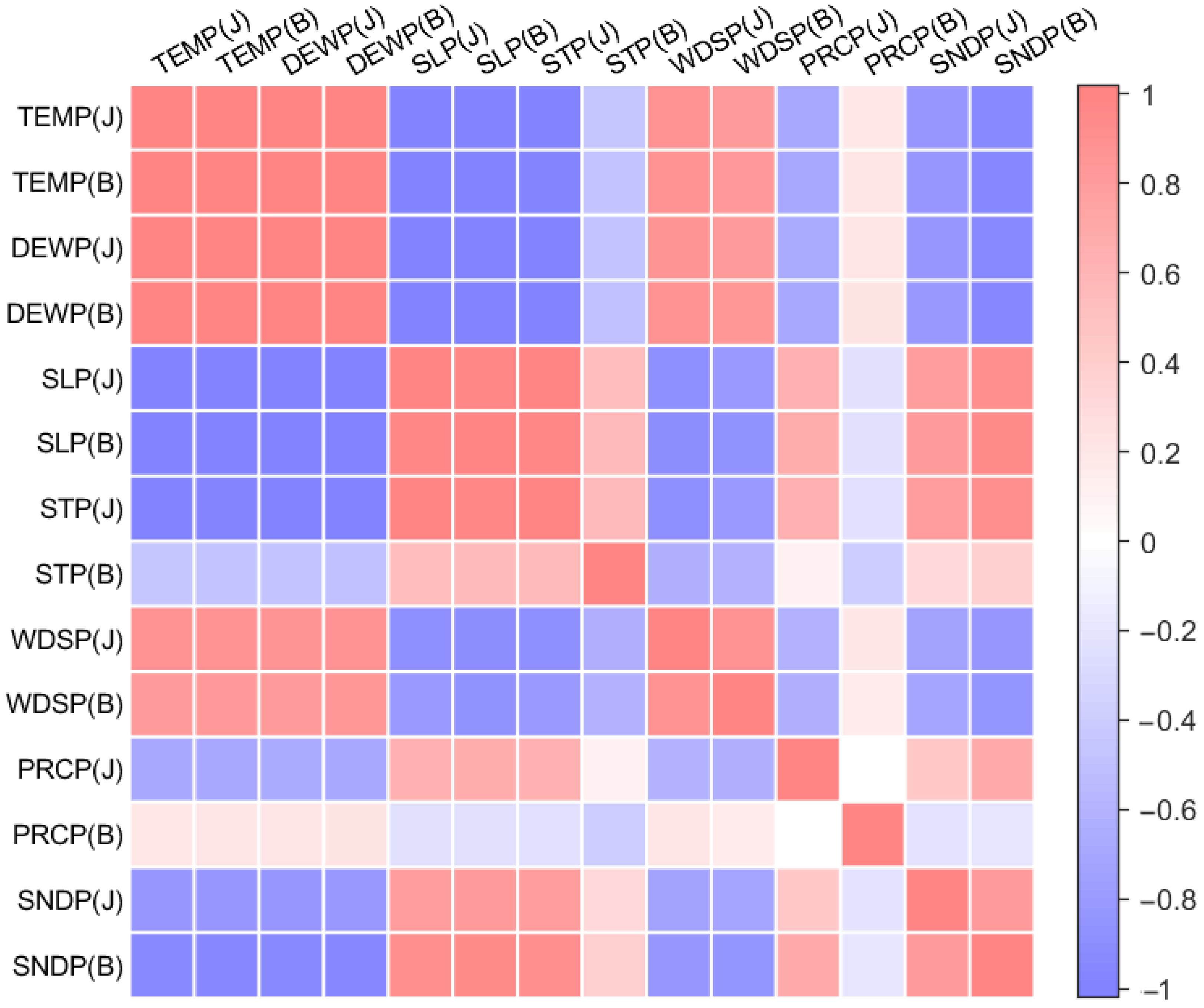
In this study, we selected 14 elements (see Table 1) from two weather stations (JINGHE and BAYANBULAK) for modeling. It can be seen from Figure 4 that quite a few of the elements had a high linear correlation, including TEMP, DEWP, and SLP. In order to reduce the impact of these factors on the model, we needed to screen the most representative factors from 14 elements.
Principal component analysis is used to reduce the dimensionality of data. On the one hand, it is necessary to reduce the data dimension as much as possible, and on the other hand, it is necessary to retain the details of the original data as much as possible. These two options have conflicting requirements for data dimensions, so a balance needs to be established between the two requirements.
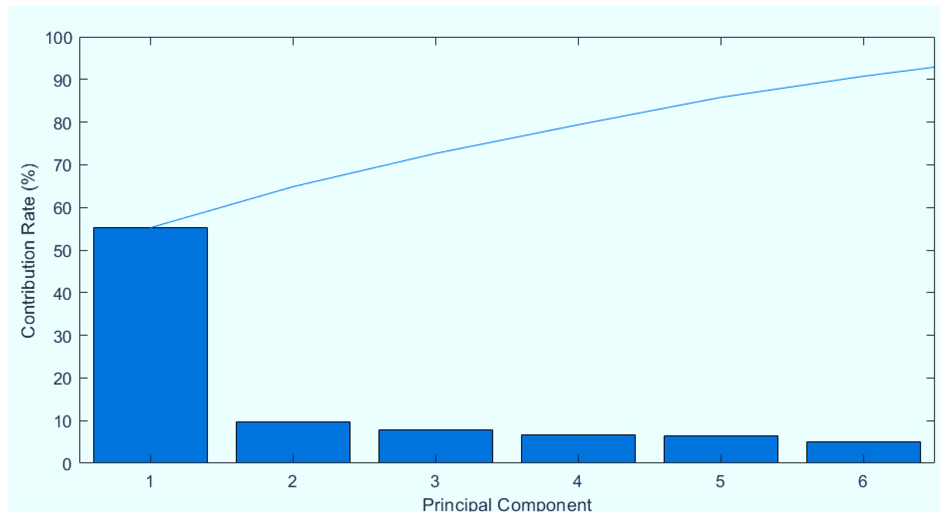
Figure 5 shows the cumulative PCA contributions. It can be seen from Figure 5 that the cumulative contribution of 6 principal components reached 90%, which means that at least 6 dimensions were needed to approximately describe most features of the original dataset.
Table 2 shows the factor analysis results. The Pearson coefficient method determines the degree of linear correlation between various elements, and the PCA method determines the minimum dimensions needed to describe the dataset. Finally, the input elements of the machine learning model were determined through the factor analysis method. The five elements of SLP(J), WDSP(J), STP(B), SNDP(B), and SNDP(J) were selected and combined with the precipitation and water level of Lianggoushan Station to form a modeling dataset.

3.2. Machine Learning Results

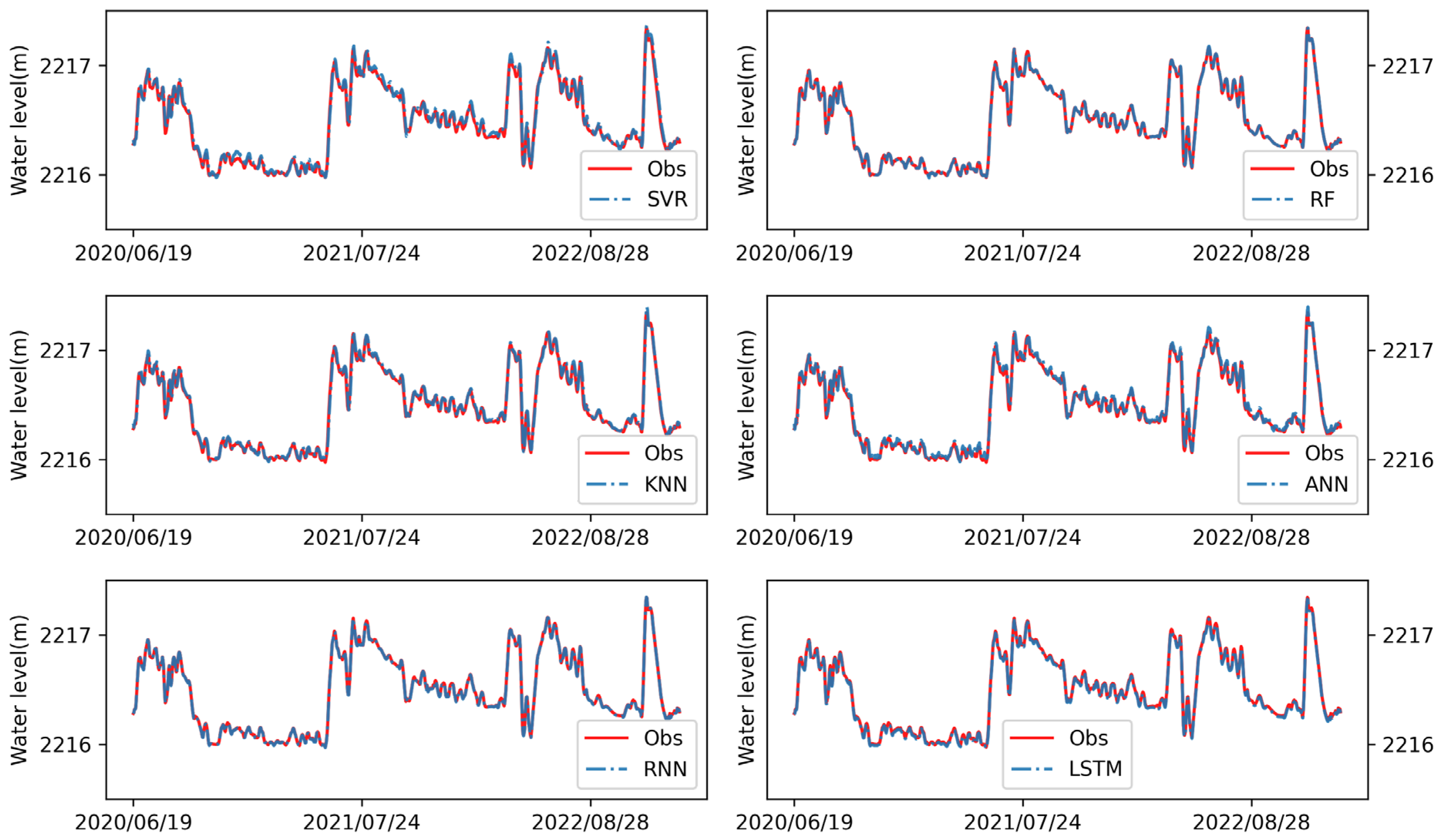
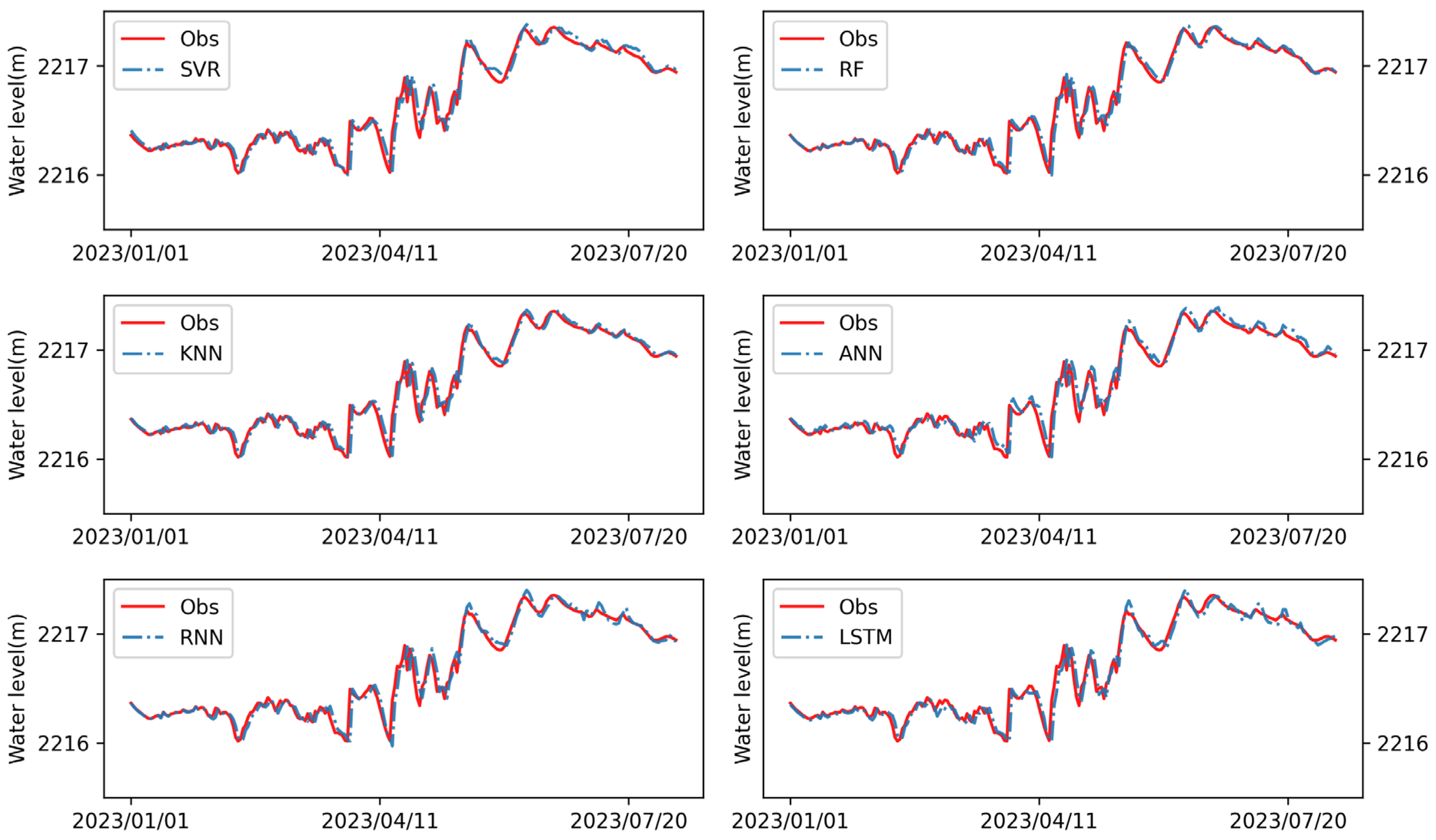
The choice of hyperparameters will have an important impact on the results of machine learning. For the 6 different models, we designed and calculated 24 sets of results. The models and parameters corresponding to each set of results are shown in Table 3. The best performance results of each machine learning method are shown in Table 4, and the water level process corresponding to training and testing is shown in Figure 6 and Figure 7.

3.3. Selection of Hyperparameters

In the SVR model, we tried 4 kinds of kernel functions, including linear (linear kernel), poly (polynomial kernel), RBF (radical basis function) and sigmoid (sigmoid tanh). As can be seen from Table 3, the simulation results of RBF were better than those of other kernel functions, and the results of sigmoid were relatively poor, which made it unsuitable for this model.
The performance of the random forest model was excellent. This study compared the results of using different numbers of estimators. From Table 3, it can be seen that the results of using 10, 50, 100, and 500 estimators were not significantly different, and the ranking of all four results was relatively high. From this set of results, it can be seen that the more estimators there were, the better the results. However, after a certain number of estimators, the improvement of the results was negligible.
The KNN performance was best in testing. It can be seen from Table 3 that fewer neighbors can produce better simulation results, so we ran some additional tests, changing the neighbors from 2 to 10 for each test. Among these results, the best result for the number of neighbors was 2. In these tests of KNN, the distance function adopted the default value ‘minkowski’, and p = 2, which is equivalent to the standard Euclidean distance.
In the ANN algorithm, in order to speed up the convergence, we used the Adam algorithm to adaptively modify the learning rate. We compared 4 kinds of activation functions, including identity, logistic, tanh, and relu, the results of relu were relatively better, so finally relu was selected as the activation function here. It can be seen from Table 3 that the more neurons, the better the simulation results of ANN. Determining a reasonable number of neurons was the key to improving the performance of ANN.
In the RNN algorithm, we used the Adam algorithm to modify the learning rate, used relu as the activation function, and mean square error (MSE) as a loss function. It can be seen from Table 3 that the performance of the RNN algorithm in training was the best among several methods, but the performance in testing was poor. In order to prevent overfitting, we added a dropout layer to the model mechanism, and the discard rate was set to 0.05; that is, we randomly discarded 5% of the data. It can be seen from Table 3 that the performance of RNN improved steadily with the increase of the number of neurons and layers.
As can be seen from Table 3, the comprehensive performance of LSTM was the best among several models. In order to better compare RNN and LSTM, we used the same parameter settings as RNN in LSTM. When the 4-layer LSTM structure was adopted and the number of hidden nodes was set to 256, 128, 64, and 32 respectively, the model achieved the best results among the 24 groups both in the training and the testing. Juna et al. believe that the number of layers of LSTM is not important, and there is little difference between using a single-layer structure and a multi-layer structure [22]. This is inconsistent with the results of this study. This may be related to the dimension of the input data. In the study of Juna et al., the dimension of input data did not exceed 10 dimensions, and the dimension of the input data for this study was 7 × 30. This leads to a more complex LSTM model structure required for optimization but this does not mean that more neurons and layers will lead to better results. When using a 4-layer LSTM structure and setting the number of hidden nodes to 1024, 512, 256, and 128, the model training RMSE changed from 0.10 to 0.13, and the test RMSE changed from 0.071 to 0.073. The results became worse.

3.4. Result Analysis

The best results of each machine learning method were selected from the 24 sets of results, and Figure 8 shows the boxplots of their error distributions during the training and testing periods. It can be seen from the figure that the median errors of LSTM and RNN were relatively close to 0 in both the training period and the test period, and these two models performed especially well in the training. In addition, the performance of the RF model was quite good, with lower errors in the test period and the training period than the SVR, KNN, and ANN models.
It can be seen from Table 4 that the results of LSTM were the best, with RMSE of 0.011 and 0.071 in the training period and testing period, and R2 of 0.999 and 0.970, respectively. The next best results were from RF, whose RMSEs in the training period and the test period were 0.012 and 0.072, respectively; R2 values were 0.999 and 0.969, respectively. From an application point of view, RF may be a better choice, because as long as the number of classifiers is set large enough, an ideal model can be obtained through training. The LSTM model requires more work on model structure design and parameter tuning.
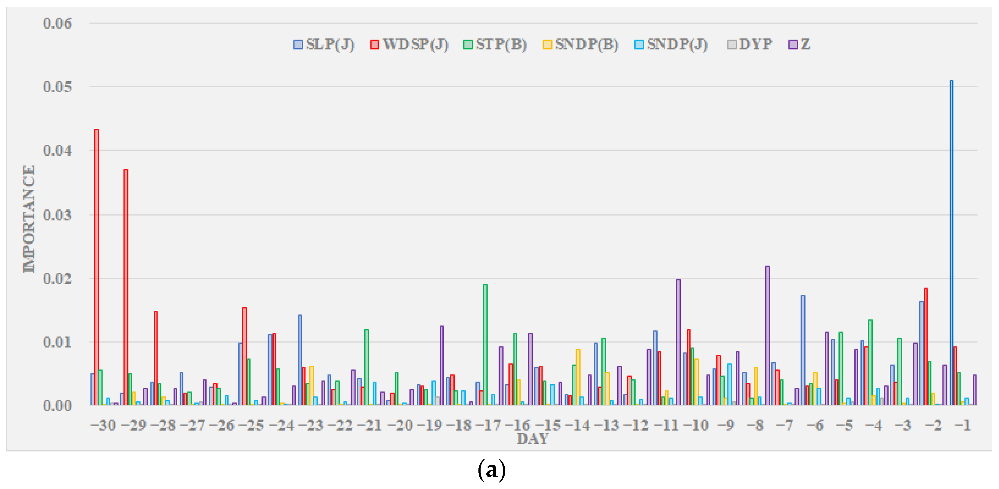
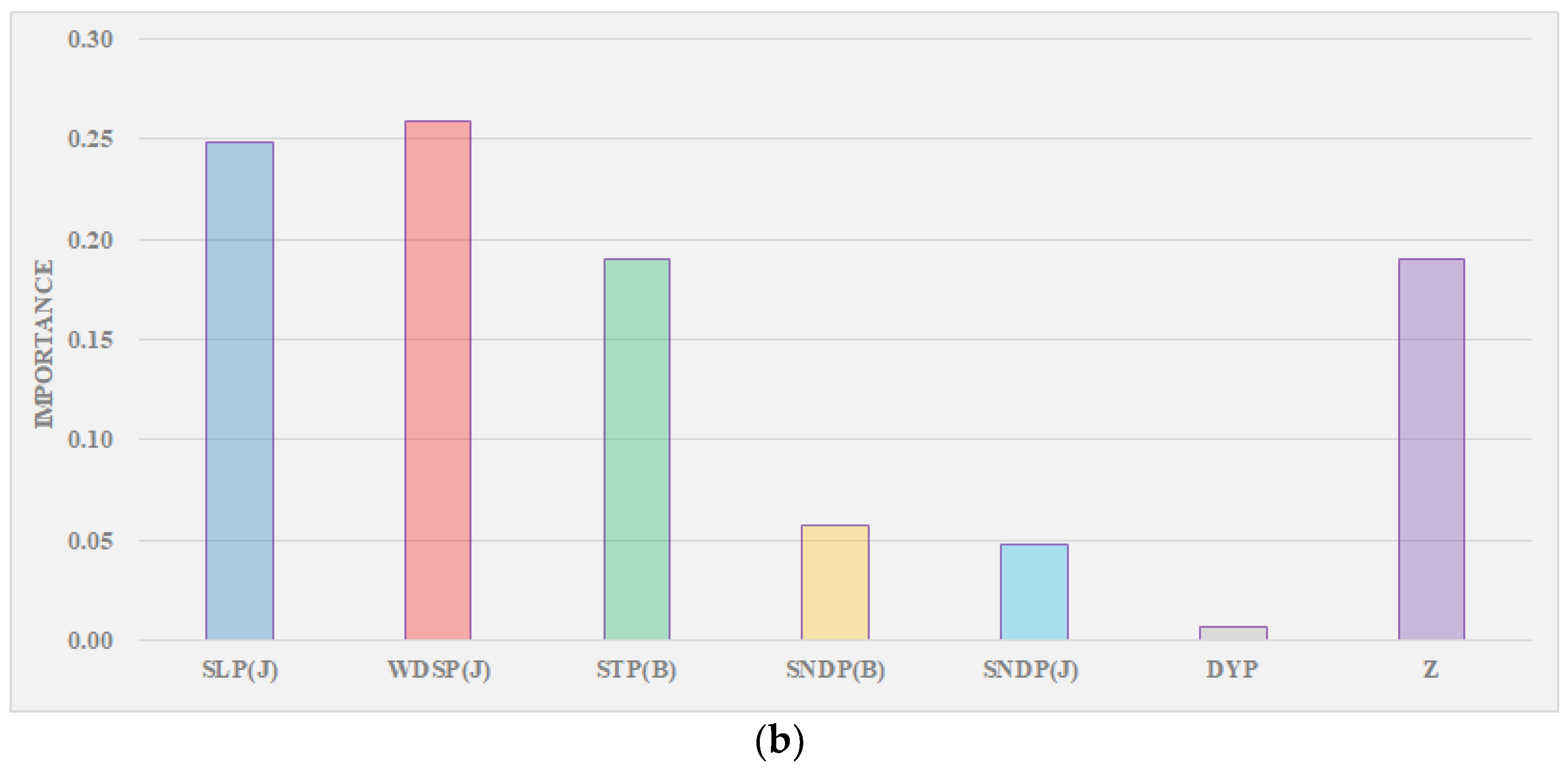
Figure 9a shows the importance of various elements in the random forest model. It can be seen from the figure that the most important thing in predicting the residual result was the average sea level pressure of the previous day, followed by the average wind speed of the 30 days ago. Figure 9b shows the cumulative importance of various elements. It can be seen from the figure that the average wind speed had the highest cumulative importance, followed by the average sea level pressure, and then the average station pressure of BAYANBULAK station and Lianggoushan station. The water level of Lianggoushan Station was less important to the model than the daily precipitation. It can also be inferred that the flood at Lianggoushan was mainly caused by snowmelt, with relatively less runoff caused by rainfall.
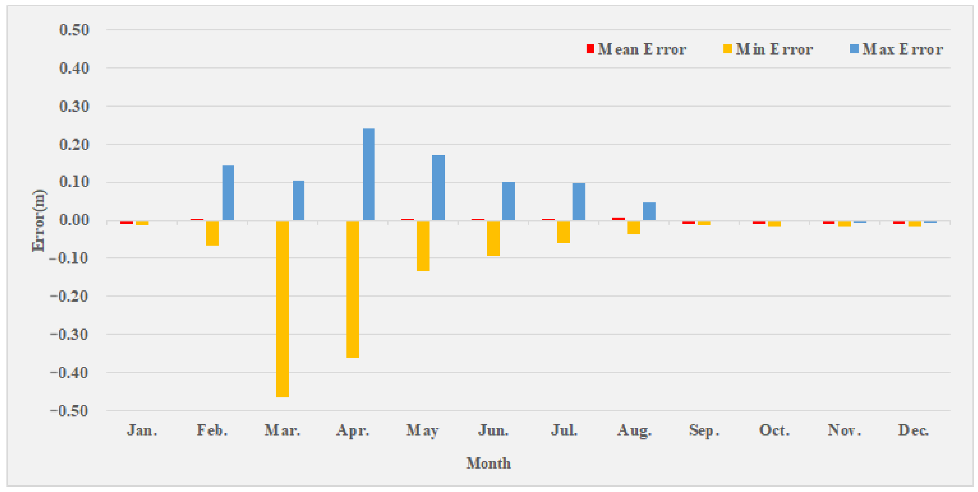
Table 5 and Figure 10 show the average error, maximum error, and minimum error of the LSTM model for each month. It can be seen from Table 5 that the monthly average water level error of the LSTM model was relatively stable, mostly not exceeding ±0.01 m. The overall error range was [−0.465, 0.240]. It can be seen from Figure 10 that the model was largest in March and April, and its performance was unstable. This period is a critical period for the annual snowmelt for glaciers in Xinjiang. This also shows that the currently selected elements cannot fully explain the process of glacier snowmelt runoff. How to optimize the error of LSTM and further reduce the error range is another direction that needs to be studied next.
In addition, it should be pointed out that the choice of fitting data has a great influence on the results. In the initial study, the first choice was to fit the water level data, and the result was so poor that it could not be put into practical use at all. After choosing the water level residual, the simulation results were significantly improved. In addition to the daily average water level, the model can also predict the daily minimum water level and daily maximum water level after simple modification.

4. Conclusions

In this study, a daily water level prediction model of the Lianggoushan catchment was constructed. Combined with the daily meteorological and hydrological observation data of the previous month, it could predict the average water level of the following day. Comparing the simulation results of SCR, RF, KNN, ANN, RNN, and LSTM, the main conclusions are as follows:
(1)
We used Pearson coefficient, principal component analysis, and factor analysis to screen input elements, screen 14 kinds of meteorological observation data from JINGHE and BAYANBULAK stations, and finally select 5 kinds of elements for modeling, including average sea level pressure, average wind speed, snow cover depth of JINGHE and average station pressure, and snow cover depth of BAYANBULAK. From the perspective of Pearson coefficient, the average temperature, average dew point, and average sea level pressure had a very high linear correlation. When constructing the model, we approximated that they were equivalent and only retained one.
(2)
SVR, RF, KNN, ANN, RNN, and LSTM were selected to construct 24 sets of models with different hyperparameters. Among all the models, LSTM had the best results, and the RMSEs in the training period and the testing period were respectively 0.011 and 0.071, and R2 values were 0.999 and 0.970, respectively. Next best were the results of RF, whose RMSEs in the training period and the test period were 0.012 and 0.072, respectively; R2 values were 0.999 and 0.969, respectively. Compared to other models, LSTM performed best, but it had more hyperparameters to optimize. From an application point of view, RF may be a better choice, because as long as the number of classifiers is set large enough, a model with good performance can be obtained. The LSTM model requires more work on model structure design and parameter optimization.
(3)
From the contribution rate results of the RF model, when the model made predictions, the contribution of meteorological elements was higher, and the contribution of rainfall in the basin was lower. From the prediction results of LSTM, the average error of each month was relatively stable, most of which did not exceed ±0.01 m, and the errors fluctuated greatly in March and April. The selection of fitting data is very important when modeling. The results obtained by directly fitting the water level were not ideal. Adjusting the model to try to fit the water level residuals (i.e., the difference between future water levels and known water levels), and calculating future water levels based on the predicted residuals, would significantly improve the accuracy of the simulation.
(4)
The purpose of this study was to explore a hydrological forecast method that can be used in practical work under limited data conditions. Hydrological sensors have been widely constructed in Xinjiang, and as time goes by, more and more hydrological data will be available for modeling. For areas with rich hydrological data, there are more and better choices when modeling. Physical models, distributed models, or combinations of different types of models can obtain richer conclusions and results. Therefore, the method proposed in this study is a temporary solution when hydrological data are limited, and subsequent research on snowmelt models and forecasting and early warning technologies in Xinjiang should be continued.

Author Contributions

Conceptualization, M.Z.; methodology, Q.M.; software, W.L.; validation, H.W.; investigation, B.H.; resources, D.L.; data curation, R.D. All authors have read and agreed to the published version of the manuscript.

Funding

This research was funded by Non-engineering Measures Operation and Maintenance for Flash Flood Prevention and Control Project of Xinjiang Production and Construction Corps (JZ120203A0522022), Flash Flood Prevention Project of Xinjiang Production and Construction Corps (JZ120203A0512022).

Data Availability Statement

Not applicable.

Conflicts of Interest

The authors declare no conflict of interest.

References

  1. Zhao, Y.; Deng, X.L.; Li, Q.; Yang, Q.; Huo, W. Characteristics of the Extreme Precipitation Events in the Tianshan Mountains in Relation to Climate Change. J. Glaciol. Geocryol. 2010, 32, 927–934. [Google Scholar]
  2. Xu, L.P.; Li, P.H.; Li, Z.Q.; Zhang, Z.Y.; Wang, P.Y.; Xu, C.H. Advances in research on changes and effects of glaciers in Xinjiang mountains. Adv. Water Sci. 2020, 31, 946–959. [Google Scholar] [CrossRef]
  3. Chen, Y.N.; Li, Z.; Fang, G.H. Changes of key hydrological elements and research progress of water cycle in the Tianshan Mountains, Central Asia. Arid. Land Geogr. 2022, 45, 1–8. [Google Scholar]
  4. Cui, M.Y.; Zhou, G.; Zhang, D.H.; Zhang, S.Q. Global snowmelt flood disasters and their impact from 1900 to 2020. J. Glaciol. Geocryol. 2022, 44, 1898–1911. [Google Scholar]
  5. Wei, T.F.; Liu, Z.H.; Wang, Y. Effect on Snowmelt Water Outflow of Snow-covered Seasonal Frozen Soil. Arid. Zone Res. 2015, 32, 435–441. [Google Scholar] [CrossRef]
  6. Wu, S.F.; Liu, Z.H.; Qiu, J.H. Analysis of the Characteristics of Snowmelt Flood and Previous Climate Snow Condition in North Xinjiang. J. China Hydrol. 2006, 26, 84–87. [Google Scholar]
  7. Huai, B.J.; Li, Z.Q.; Sun, M.P.; Xiao, Y. Snowmelt runoff model applied in the headwaters region of Urumqi River. Arid Land Geogr. 2013, 36, 41–48. [Google Scholar] [CrossRef]
  8. Muattar, S.; Ding, J.L.; Abudu, S.; Cui, C.L.; Anwar, K. Simulation of Snowmelt Runoff in the Catchments on Northern Slope of the Tianshan Mountains. Arid Zone Res. 2016, 33, 636–642. [Google Scholar] [CrossRef]
  9. Yu, Q.Y.; Hu, C.H.; Bai, Y.G.; Lu, Z.L.; Cao, B.; Liu, F.Y.; Liu, C.S. Application of snowmelt runoff model in flood forecasting and warning in Xinjiang. Arid Land Geogr. 2023, 1–15. [Google Scholar]
  10. Dang, S.Z.; Liu, C.M. Modification of SNTHERM Albedo Algorithm and Response from Black Carbon in Snow. Adv. Mat. Res. 2011, 281, 147–150. [Google Scholar] [CrossRef]
  11. Bartelt, P.; Lehning, M. A physical SNOWPACK model for the Swiss avalanche warning. Cold Reg. Sci. Technol. 2002, 35, 123–145. [Google Scholar] [CrossRef]
  12. Wang, W.C.; Zhao, Y.W.; Tu, Y.; Dong, R.; Ma, Q.; Liu, C.J. Research on Parameter Regionalization of Distributed Hydrological Model Based on Machine Learning. Water 2023, 15, 518. [Google Scholar] [CrossRef]
  13. Vafakhah, M.; Sedighi, F.; Javadi, M.R. Modeling the Rainfall-Runoff Data in Snow-Affected Watershed. Int. J. Comput. Electr. Eng. 2014, 6, 40. [Google Scholar] [CrossRef]
  14. Thapa, S.; Zhao, Z.; Li, B.; Lu, L.; Fu, D.; Shi, X.; Tang, B.; Qi, H. Snowmelt-Driven Streamflow Prediction Using Machine Learning Techniques (LSTM, NARX, GPR, and SVR). Water 2020, 12, 1734. [Google Scholar] [CrossRef]
  15. Himan, S.; Ataollah, S.; Somayeh, R.; Shahrokh, A.; Binh, T.P.; Fatemeh, M.; Marten, G.; John, J.C.; Dieu, T.B. Flash flood susceptibility mapping using a novel deep learning model based on deep belief network, back propagation and genetic algorithm. Geosci. Front. 2021, 12, 101100. [Google Scholar] [CrossRef]
  16. Wang, G.; Hao, X.; Yao, X.; Wang, J.; Li, H.; Chen, R.; Liu, Z. Simulations of Snowmelt Runoff in a High-Altitude Mountainous Area Based on Big Data and Machine Learning Models: Taking the Xiying River Basin as an Example. Remote Sens. 2023, 15, 1118. [Google Scholar] [CrossRef]
  17. Yang, R.; Zheng, G.; Hu, P.; Liu, Y.; Xu, W.; Bao, A. Snowmelt Flood Susceptibility Assessment in Kunlun Mountains Based on the Swin Transformer Deep Learning Method. Remote Sens. 2022, 14, 6360. [Google Scholar] [CrossRef]
  18. Zhou, G.; Cui, M.Y.; Li, Z.; Zhang, S.Q. Dynamic evaluation of the risk of the spring snowmelt flood in Xinjiang. Arid Zone Res. 2021, 38, 950–960. [Google Scholar]
  19. Waldmann, P. On the Use of the Pearson Correlation Coefficient for Model Evaluation in Genome-Wide Prediction. Front. Genet. 2019, 10, 899. [Google Scholar] [CrossRef]
  20. Jackson, J.E. A User’s Guide to Principal Components; Wiley: Hoboken, NJ, USA, 1992. [Google Scholar]
  21. Horn, J.L. A rationale and test for the number of factors in factor analysis. Psychnmetrica 1965, 30, 179–185. [Google Scholar] [CrossRef]
  22. Okkan, U.; Serbes, Z.A. Rainfall–runoff modeling using least squares support vector machines. Environmetrics 2012, 23, 549–564. [Google Scholar] [CrossRef]
  23. Panahi, M.; Sadhasivam, N.; Pourghasemi, H.R.; Rezaie, F.; Lee, S. Spatial prediction of groundwater potential mapping based on convolutional neural network (CNN) and support vector regression (SVR). J. Hydrol. 2020, 588, 125033. [Google Scholar] [CrossRef]
  24. Breiman, L. Random Forests. Mach. Learn. 2001, 45, 5–32. [Google Scholar] [CrossRef]
  25. Li, X.N.; Zhang, Y.J.; She, Y.J.; Chen, L.W.; Chen, J.X. Estimation of impervious surface percentage of river network regions using an ensemble leaning of CART analysis. Remote Sens. Land Resour. 2013, 25, 174–179. [Google Scholar]
  26. Juna, A.; Umer, M.; Sadiq, S.; Karamti, H.; Eshmawi, W.; Mohamed, A.; Ashraf, I. Water Quality Prediction Using KNN Imputer and Multilayer Perceptron. Water 2022, 14, 2592. [Google Scholar] [CrossRef]
  27. Lippmann, R.P. An introduction to computing with neural nets. IEEE Assp. Mag. 1988, 4, 4–22. [Google Scholar] [CrossRef]
  28. Robert, H.N. Theory of the backpropagation neural network. In Proceedings of the International Joint Conference on Neural Networks (IJCNN), Washington, DC, USA, 18–22 June 1988. [Google Scholar]
  29. Wang, S.S.; Xu, P.B.; Hu, S.Y.; Wang, K. Research on a Deep Learning Based Model for Predicting Mountain Flood Water Level in Small Watersheds. Comput. Knowl. Technol. 2022, 18, 89–91. [Google Scholar] [CrossRef]
  30. Gao, W.L.; Gao, J.X.; Yang, L.; Wang, M.J.; Yao, W.H. A Novel Modeling Strategy of Weighted Mean Temperature in China Using RNN and LSTM. Remote Sens. 2021, 13, 3004. [Google Scholar] [CrossRef]
  31. Hochreiter, S.; Schmidhuber, J. Long Short-Term Memory. Neural Comput. 1997, 9, 1735–1780. [Google Scholar] [CrossRef]
  32. Liu, X.; Zhao, N.; Guo, J.Y.; Guo, B. Prediction of monthly precipitation over the Tibetan Plateau based on LSTM neural network. J. Geo-Inf. Sci. 2020, 22, 1617–1629. [Google Scholar] [CrossRef]
Figure 1. Location of Lianggoushan catchment.
Water 15 03620 g001
Figure 2. Observed data of stations.
Water 15 03620 g002
Figure 3. Flow chart of modeling.
Water 15 03620 g003
Figure 4. Pearson correlation coefficient matrix.
Water 15 03620 g004
Figure 5. Principal Component Contribution.
Water 15 03620 g005
Figure 6. Training water level results from May 2020 to December 2022.
Water 15 03620 g006
Figure 7. Testing water level results from January 2023 to July 2023.
Water 15 03620 g007
Figure 8. Statistics of water level error. (a) Water level error in training. (b) Water level error in testing.
Water 15 03620 g008
Figure 9. Element importance. (a) The importance of elements in the first 30 days. (b) Accumulated importance of each element.
Water 15 03620 g009aWater 15 03620 g009b
Figure 10. Monthly water level error of LSTM model.
Water 15 03620 g010
Table 1. Data item details.
StationData SourceItemDescMean ValuePrecision and Unit
LianggoushanHydrological departmentZWater level2216.560.01 m
DYPPrecipitation1.80.1 mm
JINGHEGSODTEMP(J)Average temperature49.40.1 °F
DEWP(J)Average dew point30.00.1 °F
SLP(J)Average sea level pressure1021.20.1 mb
STP(J)Average station pressure981.20.1 mb
WDSP(J)Average wind speed4.10.1 knots
PRCP(J)Daily precipitation0.140.01 inches
SNDP(J)Snow cover depth0.20.1 inches
BAYANBULAKGSODTEMP(B)Average temperature26.10.1 °F
DEWP(B)Average dew point15.00.1 °F
SLP(B)Average sea level pressure1029.20.1 mb
STP(B)Average station pressure758.20.1 mb
WDSP(B)Average wind speed5.60.1 knots
PRCP(B)Daily precipitation0.050.01 inches
SNDP(B)Snow cover depth1.00.1 inches
Table 2. Factor analysis results.
ItemCom1Com 2Com 3Com 4Com 5
TEMP(J)0.910.260.11−0.21−0.16
TEMP(B)0.850.280.04−0.41−0.15
DEWP(J)0.900.210.05−0.14−0.15
DEWP(B)0.850.300.01−0.36−0.13
SLP(J)−0.95−0.160.160.080.12
SLP(B)−0.82−0.320.190.400.14
STP(J)−0.95−0.130.220.050.11
STP(B)−0.11−0.160.97−0.02−0.03
WDSP(J)0.350.70−0.080.00−0.05
WDSP(B)0.180.62−0.14−0.25−0.09
PRCP(J)−0.24−0.14−0.140.23−0.14
PRCP(B)0.050.03−0.060.01−0.02
SNDP(J)−0.26−0.10−0.030.090.78
SNDP(B)−0.45−0.140.000.580.21
Table 3. Hyperparameter settings and results.
AlgorithmSetting ItemsHyperparameterTrainingTesting
RMSER2RMSER2
SVRKernel functionkernel = linear0.0410.9850.0820.960
kernel= rbf0.0330.9900.0750.967
kernel = poly0.0360.9880.0780.964
kernel = sigmoid5884−3.2 × 1083251−6.2 × 10⁸
RFEstimator numberEstimators = 100.0140.9980.0730.969
Estimators = 500.0130.9980.0720.969
Estimators = 1000.0120.9990.0720.970
Estimators = 5000.0120.9990.0720.969
KNNNeighbor numberNeighbors = 20.0160.9970.0710.970
Neighbor = 100.0290.9920.0710.970
Neighbor = 300.0330.9900.0700.971
Neighbor = 1000.0350.9890.0700.971
ANNNumber of neurons and layers16 × 160.0380.9860.0740.968
32 × 320.0400.9850.0780.964
64 × 640.0310.9910.0750.967
256 × 2560.0220.9950.0750.967
RNNNumber of neurons and layers10240.0110.9990.0830.959
64 × 320.0100.9990.0760.966
128 × 64 × 320.0120.9990.0760.966
256 × 128 × 64 × 320.0110.9990.0750.967
LSTMNumber of neurons and layers10240.0130.9980.0760.966
64 × 320.0120.9990.0720.969
128 × 64 × 320.0120.9990.0730.968
256 × 128 × 64 × 320.0100.9990.0710.970
Table 4. Best results of each method.
AlgorithmTrainingTesting
RMSER2RMSER2
SVR0.0330.9900.0750.967
RF0.0120.9990.0720.969
KNN0.0160.9970.0710.970
ANN0.0220.9950.0750.967
RNN0.0110.9990.0750.967
LSTM0.0100.9990.0710.970
Table 5. Monthly water level errors of RF model and LSTM model.
MonthMean Water Level (m)Error of LSTM Model
MeanMinMax
Jan.2216.29−0.009−0.0140.000
Feb.2216.240.001−0.0680.144
Mar.2216.22−0.005−0.4650.102
Apr.2216.47−0.003−0.3610.240
May2216.450.000−0.1320.171
Jun.2216.970.004−0.0920.101
Jul.2216.920.002−0.0610.096
Aug.2216.740.008−0.0370.048
Sep.2216.59−0.009−0.014−0.003
Oct.2216.33−0.010−0.015−0.004
Nov.2216.33−0.011−0.018−0.007
Dec.2216.53−0.010−0.017−0.007
Disclaimer/Publisher’s Note: The statements, opinions and data contained in all publications are solely those of the individual author(s) and contributor(s) and not of MDPI and/or the editor(s). MDPI and/or the editor(s) disclaim responsibility for any injury to people or property resulting from any ideas, methods, instructions or products referred to in the content.